matrices with application
Author(s)
Wang, Q; Yao, JJ
Citation
The Annals of Statistics, 2017, v. 45 n. 1, p. 415-460
Issued Date
2017
URL
http://hdl.handle.net/10722/231315
DOI:10.1214/16-AOS1463
©Institute of Mathematical Statistics, 2017
EXTREME EIGENVALUES OF LARGE-DIMENSIONAL SPIKED FISHER MATRICES WITH APPLICATION
BYQINWENWANG ANDJIANFENGYAO University of Hong Kong
Consider twop-variate populations, not necessarily Gaussian, with co-variance matrices1and2, respectively. LetS1andS2be the correspond-ing sample covariance matrices with degrees of freedommandn. When the differencebetween1and2is of small rank compared top, mandn, the Fisher matrixS:=S−21S1is called aspiked Fisher matrix. Whenp, m andngrow to infinity proportionally, we establish a phase transition for the extreme eigenvalues of the Fisher matrix: a displacement formula showing that when the eigenvalues of(spikes) are above (or under) a critical value, the associated extreme eigenvalues ofSwill converge to some point outside the support of the global limit (LSD) of other eigenvalues (become outliers); otherwise, they will converge to the edge points of the LSD. Furthermore, we derive central limit theorems for those outlier eigenvalues ofS. The limiting distributions are found to be Gaussian if and only if the corresponding pop-ulation spike eigenvalues inaresimple. Two applications are introduced. The first application uses the largest eigenvalue of the Fisher matrix to test the equality between two high-dimensional covariance matrices, and explicit power function is found under the spiked alternative. The second application is in the field of signal detection, where an estimator for the number of signals is proposed while the covariance structure of the noise is arbitrary.
1. Introduction. Consider twop-variate populations with covariance matri-ces1and2, and letS1andS2 be the sample covariance matrices from samples of the two populations with degrees of freedommandn, respectively. When the difference between1 and2 is of finite rank, the Fisher matrixS:=S2−1S1 is called aspiked Fisher matrix. In this paper, we derive three results related to the extreme eigenvalues of the spiked Fisher matrix for general populations in the large-dimensional regime, that is, the dimension (p) grows to infinity together with the two sample sizes (m and n). Our first result is a phase transition phe-nomenon for the extreme eigenvalues ofS: a displacement formula showing that when the eigenvalues of(spikes) are above (or under) a critical value, the asso-ciated extreme eigenvalues ofS will converge to some point outside the support of the global limit (LSD) of other eigenvalues (become outliers), and the loca-tion of this limit only depends on the corresponding populaloca-tion spike of and
Received April 2015; revised March 2016.
MSC2010 subject classifications.Primary 62H12; secondary 60F05.
Key words and phrases.Large-dimensional Fisher matrices, spiked Fisher matrix, spiked popu-lation model, extreme eigenvalue, phase transition, central limit theorem, signal detection, high-dimensional data analysis.
two dimension-to-sample-size ratios; otherwise, they will converge to the edge points of the LSD. The second result is on the second-order behavior of those out-lier eigenvalues ofS. We show that after proper normalization, a packet of those outlier eigenvalues (corresponding to the same spike in) converge to the eigen-values’ distribution of some structured Gaussian random matrix. In particular, the limiting distribution of the outlier eigenvalue of S (after normalization) is Gaus-sian if and only if the corresponding spike inis simple. Finally, as an extension, we consider the joint distribution of all those outlier eigenvalues (correspond to different spikes in ) as a whole, and it is shown that those outlier eigenvalues (after normalization) converge to the eigenvalues’ distribution of some block ran-dom matrix, whose structure can be fully identified. Also as a special case, if all the spikes inare simple, then the joint distribution of the outlier eigenvalues of
Sis multivariate Gaussian.
There exists a vast literate on the spectral analysis of multivariate Fisher matri-ces under the assumption that both populations are Gaussian and share the same covariance matrix, that is,1=2. The joint distribution of the eigenvalues of the corresponding Fisher matrix S was first simultaneously and independently pub-lished in 1939 by R. A. Fisher, S. N. Roy, P. L. Hsu and M. A. Girshick. Later in 1980,Wachter(1980) finds a deterministic limit, the celebrated Wacheter distribu-tion, for the empirical measure of these eigenvalues when the dimensionpgrows to infinity proportionally with the degrees of freedommandn(large-dimensional regime). Wachter’s result has been later extended to non-Gaussian populations us-ing the tools from the random matrix theory and two early examples of such ex-tensions areSilverstein(1985) andBai, Yin and Krishnaiah(1987).
In this paper, we are also interested in the large-dimensional regime, while al-lowing 1 and 2 to be separated by a (finite) rank-M matrix . Besides, the two populations can have arbitrary distributions other than Gaussian. From the perturbation theory, whenM is a fixed integer whilep,mandngrow to infinity proportionally, the empirical measure of the p eigenvalues ofS will be affected by a difference of order M/p (→0), so that its limit remains the Wachter dis-tribution. Therefore, our main concern is the local asymptotic behaviors of the
M extreme eigenvalues of S (other than the global limit). In a recent preprint
Dharmawansa, Johnstone and Onatski (2014), by assuming both population are Gaussian and M=1, these authors show that, when the norm of the rank-1 dif-ference(spike) exceeds a phase transition threshold, the asymptotic behavior of the log-ratio of the joint density of these characteristic roots under a local deviation from the spike depends only on the largest eigenvaluelp,1and the statistical exper-iment of observing all the eigenvalues is locally asymptotically normal (LAN). As a by-product of their analysis, the authors also establish joint asymptotic normal-ity of a few of the largest eigenvalues when the corresponding spikes in(with
M >1) exceed the phase transition threshold. The analysis given in this refer-ence highly relies on the Gaussian assumption so that the joint density function of the eigenvalues has indeed an explicit form, and the main results are obtained via
an accurate asymptotic approximation of the log-ratio of these density functions. Therefore, one of the main objectives of our work is to develop a general theory without such Gaussian assumption. It is thus apparent that the joint density of the eigenvalues of the Fisher matrixShas then no more an analytic formula and new techniques are needed to solve the questions.
Our approach relies on the tools borrowed from the theory of random matrices. A methodology particularly successful both in theory and applications within this approach relies on thespiked population modelcoined inJohnstone(2001). This model assumes the population covariance matrix has the structurep=Ip+
where the rank of is M (M is a fixed integer). Again for small rankM, the empirical eigenvalue distribution of the corresponding sample covariance matrix remains the standard Marˇcenko–Pastur law. What makes a difference is the local asymptotic behaviors of the extreme sample eigenvalues. For example, the fluctu-ation of largest eigenvalues of a sample covariance matrix from a complex spiked Gaussian population is studied inBaik, Ben Arous and Péché(2005), where the authors uncover a phase transition phenomenon: the weak limit and the scaling of these extreme eigenvalues are different depending on whether the eigenvalues of
(spikes) are above, equal or below a critical value, situations refereed as super-critical, criticalandsub-critical, respectively. InBaik and Silverstein(2006), the authors consider the spiked population model with general populations (not nec-essarily Gaussian). For the almost sure limits of the extreme sample eigenvalues, they find that if a population spike (in) is large or small enough, the correspond-ing spiked sample eigenvalues will converge to a limit outside the support of the limiting spectrum (becomeoutliers). InPaul(2007), a CLT is established for these outliers, that is, the super-critical case, under the Gaussian assumption and assum-ing that population spikes are simple (multiplicity 1). The CLT for super-critical outliers with general populations and arbitrary multiplicity numbers is developed inBai and Yao(2008). Joint distributions for the outlier sample eigenvalues and eigenvectors can be found inShi(2013) andWang, Su and Yao(2014). A recent related application to high-dimensional regression can be found inKargin(2015). Within the theory of random matrices, the techniques we use in this paper for spiked models are closely connected to other random matrix ensembles through the concept of small-rank perturbations. Theories on perturbed Wigner matrices can be found inPéché(2006),Féral and Péché(2007),Capitaine, Donati-Martin and Féral
(2009),Pizzo, Renfrew and Soshnikov(2013) andRenfrew and Soshnikov(2013). In a more general setting of finite-rank perturbation including both the additive and the multiplicative one, referees includeBenaych-Georges and Nadakuditi(2011),
Benaych-Georges, Guionnet and Maida(2011) andCapitaine(2013).
Apart from the theoretical results, we also propose two applications both in high-dimensional hypothesis testing and signal detection, respectively. The first application uses the largest eigenvalue of the Fisher matrix to test the following hypotheses:
where is a nonnegative definite matrix of rank M. Under this spiked alterna-tiveH1, explicit formula for the power function is derived. Our second application is to propose an estimator for the number of signals based on noisy observations. Other than the existing approaches [see, e.g.,Kritchman and Nadler(2008),Nadler
(2010),Passemier and Yao(2012,2014)], our method allows the covariance struc-ture of the noise to be arbitrary.
The rest of the paper is organized as follows. First, in Section2, the exact setting of the spiked Fisher matrixS=S2−1S1is introduced. Then in Section3, we estab-lish the phase transition phenomenon for the extreme eigenvalues ofS: a displace-ment formula is found as well as the transition boundary is explicitly obtained. Next, CLTs for those outlier eigenvalues fluctuating around their limit (i.e., in the super-critical case) are established first in Section4for one group of sample eigen-values corresponding to a same population spike, and then in Section6for all the groups jointly. Section5contains numerical illustrations that demonstrate the finite sample performance of our results. In Section 7, we develop in detail two appli-cations in high-dimensional statistics. Proofs of the main theorems (Theorems3.1
and4.1) are included in Section8while some technical lemmas are grouped in the
Appendix.
2. Spiked Fisher matrix and preliminary results. In what follows, we will assume that2=Ip. This assumption does not lose any generality since the
eigen-values of the Fisher matrixS=S2−1S1are invariant under the transformation
S1→2−1/2S12−1/2, S2→2−1/2S22−1/2. (2.1)
Also we will writepfor1to signify the dependence on the dimensionp. Let
Z=(z1, . . . , zn)=(zij)1≤i≤p,1≤j≤n
(2.2) and
W =(w1, . . . , wm)=(wkl)1≤k≤p,1≤l≤m
(2.3)
be two independent arrays, with respective sizep×nandp×m, of independent real-valued random variables with mean 0 and variance 1. Now suppose we have two samples{zi}1≤i≤nand{xi=p1/2wi}1≤i≤m, where{zi}and{wi}are given by
(2.2) and (2.3), andpis a rankM (Mis a fixed integer) perturbation ofIp, that
is, (2.4) p= M 0 0 Ip−M .
Here,Mis aM×Mcovariance matrix, containingknonzero and nonunit
eigen-values (ai), with multiplicity numbers (ni) (n1 + · · · +nk =M). That is, M
has the eigen-decompositionUdiag(a1, . . . , a 1
n1
, . . . , ak, . . . , a k nk
)U∗, where U is a
The sample covariance matrices of the two observations{xi}and{zi}are (2.5) S1= 1 m m l=1 xlxl∗= 1 mXX ∗=1/2 p 1 mW W ∗1/2 p and (2.6) S2= 1 n n j=1 zjzj∗= 1 nZZ ∗, respectively.
Throughout the paper, we consider an asymptotic regime of Marˇcenko–Pastur-type, that is,
p∧n∧m→ ∞, yp:=p/n→y∈(0,1) and
(2.7)
cp:=p/m→c >0.
Recall that theempirical spectral distribution(ESD) of ap×pmatrixAwith eigenvalues{λj}is the distributionp−1 jp=1δλj whereδa denotes the Dirac mass ata. Since the total rankM generated by thek spikes is fixed, the ESD ofSwill have the same limit (LSD) as there were no spikes inp. This limiting spectral
distribution, which is the celebrated Wachter distribution, has been known for a long time.
PROPOSITION2.1. For the Fisher matrixS=S2−1S1 with the sample
covari-ance matricesSi’s given in(2.5)–(2.6),assume that the dimensionpand the two sample sizesn, mgrow to infinity proportionally as in(2.7).Then almost surely,
the ESD ofSweakly converges to a deterministic distributionFc,ywith a bounded support[α, β]and a density function given by
fc,y(x)= ⎧ ⎪ ⎨ ⎪ ⎩ (1−y)√(β−x)(x−α) 2π x(c+xy) , whenα≤x≤β, 0, otherwise, (2.8) where α= 1−√ c+y−cy 1−y 2 and β= 1+√ c+y−cy 1−y 2 . (2.9)
Furthermore,ifc >1,thenFc,y has a point mass1−1/cat the origin.Also,the Stieltjes transforms(z)ofFc,y equals
s(z)= 1 zc− 1 z −c(z(1−y)+1−c)+2zy−c (1−c+z(1−y))2−4z 2zc(c+zy) , (2.10) z /∈ [α, β].
REMARK 2.1. Assuming both populations are Gaussian, Wachter (1980), Theorem 3.1, derives the limiting distribution for roots of the determinental equa-tion,
mS1−x2
(mS1+nS2)=0, x∈R.
The continuous component of the distribution has a compact support[A2, B2]with density function proportional to {(x −A2)(B2 −x)}1/2/{x(1−x2)}. It can be readily checked that by the change of variable z=cx2/{y(1−x2)}, the density of the continuous component of the LSD of S is exactly (2.8). The validity of this limit for general populations (nonnecessarily Gaussian) is due toSilverstein
(1985) andBai, Yin and Krishnaiah(1987).
3. Phase transition of the extreme eigenvalues ofS=S2−1S1. In this
sec-tion, we establish a phase transition phenomenon for the extreme eigenvalues of
S=S2−1S1, that is, when a population spike ai with multiplicity ni is larger (or
smaller) than a critical value, a packet ofni corresponding sample eigenvalues of Swill jump outside the support [α, β]of its LSDFc,y and converge all to a fixed
limitφ(ai), which is called the displacement of the population spikeai. Otherwise,
these associated sample eigenvalues will converge to one of the edgesα andβ. By assumption, the k population spike eigenvalues {ai} are all positive and
nonunit. We order them with their multiplicities in descending order together with thep−M unit eigenvalues as
a1= · · · =a1> a2= · · · =a2>· · ·> ak0= · · · =ak0>1= · · · =1
(3.1)
> ak0+1= · · · =ak0+1>· · ·> ak= · · · =ak.
That is,k0 of these population spike eigenvalues are larger than 1 while the other
k−k0are smaller. Let
Ji= [n1+ · · · +ni−1+1, n1+ · · · +ni], 1≤i≤k0, p−(ni+ · · · +nk)+1, p−(ni+1+ · · · +nk) , k0< i≤k. Notice that the cardinality of eachJi isni. Next, the sample eigenvalues{lp,j}of
the Fisher matrixS2−1S1 are also sorted in the descending order aslp,1≥lp,2 ≥
· · · ≥lp,p. Therefore, for each spike eigenvalueai, there areni associated sample
eigenvalues {lp,j, j ∈Ji}. The phase transition for these extreme eigenvalues is
given in the following Theorem3.1.
THEOREM3.1. For the Fisher matrixS=S2−1S1with the sample covariance
matricesSi’s given in(2.5)–(2.6),assume that the dimensionpand the two sample sizesn, mgrow to infinity proportionally as in(2.7).Then for any spike eigenvalue
ai (i=1, . . . , k),it holds that for allj∈Ji,lp,j almost surely converges to a limit λi= ⎧ ⎪ ⎪ ⎨ ⎪ ⎪ ⎩ φ(ai), |ai−γ|> γ √ c+y−cy, β, 1< ai≤γ{1+√c+y−cy}, α, γ{1−√c+y−cy} ≤ai<1, (3.2) whereγ :=1/(1−y)∈(1,∞)and φ(ai)= ai(ai+c−1) ai−aiy−1 (3.3)
is the displacement of the population spikeai.
The proof of this Theorem is postponed to Section8.1.
REMARK 3.1. Theorem 3.1states that when the population spikeai is large
enough (ai> γ{1+√c+y−cy}) or small enough (ai< γ{1−√c+y−cy}),
the corresponding extreme sample eigenvalues of the spiked Fisher matrix will converge toφ(ai), which is located outside the support[α, β]of its LSD.
Other-wise, they converge to one of its edgesαandβ. This phenomenon is depicted in Figure1for understanding.
REMARK 3.2. Using the notationγ =1/(1−y), the functionφ(x) in (3.3) could be expressed as
(3.4) φ(x)=γ x(x−1+c)
x−γ , x=γ ,
which is a rational function with a single pole atx=γ. And the function asymp-totically equals tog(x)=γ (x+c−1+γ )when|x| → ∞. On the other hand, since φ(γ{1−√c+y−cy})=α and φ(γ{1+√c+y−cy})=β, it can be checked that the pointsA(γ{1−√c+y−cy, α})andB(γ{1+√c+y−cy, β})
are exactly the two extreme points for the functionφ. An example ofφ(x) with parameters(c, y)=(15,12)is illustrated in Figure2.
REMARK3.3. It is worth observing that wheny→0, theφ(x)function tends to the function well known in the literature for similar transition phenomenon of a spiked sample covariance matrix, that is,
lim
y→0φ(x)=x+
cx
x−1, x=1, (3.5)
see, for example, theψ-function in Figure 4 ofBai and Yao(2012). These func-tions [(3.4) and (3.5)] share a same shape; however, the pole here equals 1, which is smaller than the poleγ =1/(1−y) [in (3.4)] for the case of a spiked Fisher matrix.
FIG. 1. Phase transition of the extreme eigenvalues of the spiked Fisher matrix:upper-left panel: when 1< ai ≤γ{1+√c+y−cy}, the limit of the corresponding extreme sample eigenvalue
{lp,j, j∈Ji}isβ;upper-right panel:whenai> γ{1+√c+y−cy}, the limit of{lp,j, j∈Ji} is larger than β [located at λi=φ(αi)]; lower-left panel:when γ{1−√c+y−cy} ≤ai<1, the limit of{lp,j, j∈Ji}isα;lower-right panel:when0< ai < γ{1−√c+y−cy},the limit of
{lp,j, j∈Ji}is smaller thanα[located atλi=φ(αi)].
REMARK3.4. As said in theIntroduction, this phase transition phenomenon has already been established in a preprint Dharmawansa, Johnstone and Onatski
(2014) (their Proposition 5) under Gaussian assumption and using a completely different approach. Theorem3.1proves that such a phase transition phenomenon is indeed universal.
4. Central limit theorem for the outlier eigenvalues ofS2−1S1. The aim of
this section is to give a CLT for theni-packed outlier eigenvalues: √ plp,j−φ(ai), j∈Ji . DenoteU=U1 U2 · · · Uk
, where eachUi is a matrix of sizeM×ni that
corresponds to the spike eigenvalueai.
THEOREM 4.1. Assume the same assumptions as in Theorem3.1and in ad-dition, the variables (zij) [in(2.2)] and(wkl) [in(2.3)]have the same first four moments and denotev4 as their common fourth moment:
FIG. 2. Example of the functionφ(x)with(c, y)=(15,12).Its pole is atx=2.When|x| → ∞,
φ(x)is getting close to the equationg(x)=2x+125 (see the red line).The two extreme points are at
A(0.450,0.203)andB(3.549,12.597),meaning that critical values for spikes are0.450and3.549 while the support of the LSD is[0.203,12.597].
Then for any population spike ai satisfying |ai − γ| > γ√c+y−cy, the normalized ni-packed outlier eigenvalues of S2−1S1:
√p{l
p,j −φ(ai), j ∈ Ji} converge weakly to the distribution of the eigenvalues of the random matrix −Ui∗R(λi)Ui/(λi).Here, (λi)= (1−ai−c)(1+ai(y−1))2 (ai−1)(−1+2ai+c+ai2(y−1)) , (4.1)
R(λi)=(Rmn) is a M×M symmetric random matrix, made with independent Gaussian entries of mean zero and variance
Var(Rmn)= 2θi+(v4−3)ωi, m=n, θi, m=n, (4.2) where ωi= ai2(ai+c−1)2(c+y) (ai−1)2 , (4.3) θi= ai2(ai+c−1)2(cy−c−y) −1+2ai+c+ai2(y−1) . (4.4)
REMARK 4.1. Notice that the result above involves the ith block Ui of the
eigen-matrix U. When the spike ai is simple, Ui is unique up to its sign, then Ui∗R(λi)Ui is uniquely determined. But whenai has multiplicities greater than 1, Uiis not unique; actually, any rotation ofUican be an eigenvector corresponding
toai. But, according to LemmaA.1in theAppendix, such a rotation will not affect
the eigenvalues of the matrixUi∗R(λi)Ui.
Next, we consider a special case whereM is diagonal (U=IM), with distinct
eigenvalues ai, that is, M=kand ni=1 for all 1≤i≤M. Using the previous
result of Theorem4.1, it can be shown that after normalization, the outlier eigen-valueslp,i ofS2−1S1are asymptotically Gaussian when|ai−γ|> γ√c+y−cy.
PROPOSITION4.1. Under the same assumptions as in Theorem3.1,with ad-ditional conditions that M is diagonal and all its eigenvalues ai (1≤i≤M) are simple,we have when|ai−γ|> γ√c+y−cy,the outlier eigenvaluelp,i of S2−1S1 is asymptotically Gaussian: √ p lp,i− ai(ai−1+c) ai−1−aiy =⇒N0, σi2, where σi2=2a 2 i(cy−c−y)(ai−1)2(−1+2ai+c+a2i(y−1)) (1+ai(y−1))4 +(v4−3)· ai2(c+y)(−1+2ai+c+a2i(y−1))2 (1+ai(y−1))4 .
PROOF. Under the above assumptions, the random matrix −Ui∗R(λi)Ui
re-duces to −R(λi)(i, i), which is a Gaussian random variable of mean zero and
variance 2θi+(v4−3)ωi= 2ai2(ai+c−1)2(cy−c−y) −1+2ai+c+ai2(y−1) +(v4−3)· ai2(ai+c−1)2(c+y) (ai−1)2 .
Therefore, combining with the value ofδ(λi)in (4.1) we have √ p lp,i− ai(ai−1+c) ai−1−aiy =⇒N0, σi2, where σi2=2a 2 i(cy−c−y)(ai−1)2(−1+2ai+c+a2i(y−1)) (1+ai(y−1))4 +(v4−3)· ai2(c+y)(−1+2ai+c+a2i(y−1))2 (1+ai(y−1))4 .
The proof of Proposition4.1is complete.
REMARK 4.2. Notice that when the observations are standard Gaussian, we havev4=3, then the above theorem reduces to
√ p lp,i− ai(ai−1+c) ai−1−aiy =⇒N 0,2a 2 i(ai−1)2(cy−c−y)(−1+2ai+c+a 2 i(y−1)) (1+ai(y−1))4 ,
which is exactly the result in Dharmawansa, Johnstone and Onatski (2014); see setting 1 in their Proposition 11.
5. Numerical illustrations. In this section, numerical results are provided to illustrate the results of our Theorem 4.1 and Proposition 4.1. We fix p =200,
T = 1000, n= 400 with 1000 replications, thus y =1/2 and c =1/5. The critical interval is then [γ −γ√c+y−cy, γ +γ√c+y−cy] = [0.45,3.55] and the limiting support [α, β] = [0.2,12.6]. Consider k=3 spike eigenvalues
(a1, a2, a3)=(20,0.2,0.1) with respective multiplicity (n1, n2, n3)=(1,2,1). Letl1≥ · · · ≥lp be the ordered eigenvalues of the Fisher matrixS2−1S1. We are particularly interested in the distributions ofl1, (lp−2, lp−1)andlp, which
corre-sponds to the spike eigenvaluesa1,a2 anda3, respectively.
5.1. Case ofU =I4. In this subsection, we consider a simple case that U=
I4. Therefore, following Theorem4.1, we have:
• forj=1, p,√p{lj−φ(ai)} →N (0, σi2). Here, forj=1,i=1,φ(a1)=42.67 and σ12 =4246.8+1103.5(v4 −3); and for j =p, i =3, φ(a3)=0.07 and
σ32=7.2×10⁻³+3.15×10⁻³(v4−3);
• for j =p−2, p−1 and i=2, the two-dimensional random vector √p{lj − φ(a2)} converges to the eigenvalues of the random matrix −(λRmn
2). Here, φ(a2)=0.13,(λ2)=1.45 andRmn is the 2×2 symmetric random matrix,
made with independent Gaussian entries of mean zero and variance given by (5.1) Var(Rmn)= 2θ2+(v4−3)ω2 =0.04+0.016(v4−3) , m=n, θ2(=0.02), m=n.
Simulations are conducted to compare the distributions of the empirical extreme eigenvalues with their limits.
5.1.1. Gaussian case. First, we assume all thezij andwij are i.i.d. standard
Gaussian, thus v4−3=0. And according to (5.1), Rmn/ √
0.04 is the standard 2×2 Gaussian Wigner matrix (GOE). Therefore, we have:
FIG. 3. Upper panels show the empirical densities ofl1 andlp (solid lines,after centralization and scaling)compared to their Gaussian limits(dashed lines).Lower panels show contour plots of empirical joint density function of(lp−2, lp−1)(left plot,after centralization and scaling)and contour plots of their limits(right plot).Both the empirical and limit joint density functions are displayed using the two-dimensional kernel density estimates.Samples are draw from i.i.d.standard Gaussian distribution withU=I4.The replication number is1000.
• √p{l1−42.67} →N (0,4246.8),
• √p{lp−0.07} →N (0,7.2×10−3),
• the two-dimensional random vector√p{lp−2−0.13, lp−1−0.13}converges to the eigenvalues of the random matrix−0.138·W; here,W is a 2×2 GOE.
We compare the empirical distributions with their limits in Figure 3. The upper panels show the empirical kernel density estimates (in solid lines) of
√
p{l1−42.67}and√p{lp−0.07}from 1000 independent replications, compared
to their Gaussian limitsN (0,4246.8)andN (0,7.2×10−3), respectively (dashed lines). When considering the empirical distribution of the two-dimensional random
vector√p{lp−2−0.13, lp−1−0.13}, we run the two-dimensional kernel density estimation from 1000 independent replications and display their contour lines (see the lower-left panel of the figure), while the lower-right panel shows the contour lines of the kernel density estimation of the eigenvalues of the 2×2 random matrix
−0.138·GOE(their limits).
5.1.2. Binary case. Second, we assume all the zij and wij are i.i.d. binary
variables taking values {1,−1} with probability 1/2, and in this case we have
v4=1. Similarly, we have:
• √p{l1−42.67} →N (0,2039.8),
• √p{lp−0.07} →N (0,9×10⁻⁴),
• the two-dimensional random vector √p{lp−2−0.13, lp−1−0.13} converges to the eigenvalues of the random matrix −Rmn/1.45. Here, Rmn is the 2×2
symmetric random matrix, made with independent Gaussian entries of mean zero and variance
Var(Rmn)=
0.008, m=n,
0.02, m=n.
Figure4compares the empirical distributions with their limits in this binary case. The upper panels show the empirical kernel density estimates of√p{l1−42.67} and√p{lp−0.07}from 1000 independent replications (in solid lines), compared
to their Gaussian limits (in dashed lines). Also, the lower panel shows the contour lines of the empirical joint density of the√p{lp−2−0.13, lp−1−0.13}(the left plot), with the right plot displaying the contour lines of their limit.
5.2. Case of general U. In this subsection, we consider the following nonunit orthogonal matrix: U= ⎛ ⎜ ⎜ ⎜ ⎜ ⎜ ⎜ ⎜ ⎝ 1 0 0 0 0 1 0 0 0 0 √1 2 1 √ 2 0 0 √1 2 −1 √ 2 ⎞ ⎟ ⎟ ⎟ ⎟ ⎟ ⎟ ⎟ ⎠ , (5.2)
that is, we have
U1= ⎛ ⎜ ⎜ ⎝ 1 0 0 0 ⎞ ⎟ ⎟ ⎠, U2= ⎛ ⎜ ⎜ ⎜ ⎜ ⎜ ⎜ ⎜ ⎝ 0 0 1 0 0 √1 2 0 √1 2 ⎞ ⎟ ⎟ ⎟ ⎟ ⎟ ⎟ ⎟ ⎠ , U3= ⎛ ⎜ ⎜ ⎜ ⎜ ⎜ ⎜ ⎜ ⎝ 0 0 1 √ 2 −1 √ 2 ⎞ ⎟ ⎟ ⎟ ⎟ ⎟ ⎟ ⎟ ⎠ .
FIG. 4. Upper panels show the empirical densities ofl1 andlp (solid lines,after centralization and scaling)compared to their Gaussian limits(dashed lines).Lower panels show contour plots of empirical joint density function of(lp−2, lp−1)(left plot,after centralization and scaling)and contour plots of their limits(right plot).Both the empirical and limit joint density functions are displayed using the two-dimensional kernel density estimates.Samples are draw from i.i.d.binary distribution withU=I4.The replication number is1000.
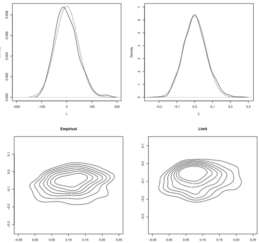
Since Gaussian distribution is invariant under orthogonal transformation, we only consider the case that all thezij andwij are i.i.d. binary variables taking values {1,−1}with probability 1/2, with all the other settings the same as in Section5.1. Then according to Theorem4.1, we have:
• √p{l1−42.67} →N (0,2039.8),
• √p{lp−0.07} →N (0,0.004),
• the two-dimensional random vector√p{lp−2−0.13, lp−1−0.13}converges to the eigenvalues of the random matrix −U2∗R(λ2)U2/1.45. Here, R(λ2) is the 4×4 symmetric random matrix, made with independent Gaussian entries of
FIG. 5. Upper panels show the empirical densities ofl1andlp(solid lines,after centralization and scaling)compared to their Gaussian limits(dashed lines).Lower panels show contour plots of em-pirical joint density function of(lp−2, lp−1)(left plot,after centralization and scaling)and contour plots of their limits(right plot).Both the empirical and limit joint density functions are displayed using the two-dimensional kernel density estimates.Samples are from i.i.d.binary distribution with
Ugiven by(5.2).The replication number is1000.
mean zero and variance
Var(Rmn)=
0.008, m=n,
0.02, m=n.
Figure5 compares the empirical distributions with their limits in this general U
case. The upper panels show the empirical kernel density estimates of √p{l1− 42.67} and √p{lp −0.07} from 1000 independent replications (in solid lines),
compared to their Gaussian limits (in dashed lines). Also, the lower panel of the figure shows the contour lines of the empirical joint density of √p{lp−2−
0.13, lp−1−0.13}(the lower-left plot), with the lower-right plot showing the con-tour lines of their limit.
6. Joint distribution of the outlier eigenvalues. In the previous section, we have obtained the following result for the outlier eigenvalues: theni-dimensional
real random vector√p{lp,j−λi, j∈Ji}converges to the distribution of the
eigen-values of a random matrix−Ui∗R(λi)Ui/(λi). It is in fact possible to derive their
joint distribution, that is, the limit of theM-dimensional real random vector ⎛ ⎜ ⎝ √p{l p,j1−λ1, j1∈J1} .. . √ p{lp,jk−λk, jk∈Jk} ⎞ ⎟ ⎠ (6.1)
if all the spike eigenvaluesai are above (or below) the phase transition threshold.
Such joint convergence result is useful for inference procedures where consecutive sample eigenvalues are used such as their differences or ratios; see, for example,
Onatski(2009) andPassemier and Yao(2014).
THEOREM6.1. Assume the same conditions as in Theorem4.1holds and all the population spikesai satisfy the condition|ai−γ|> γ√c+y−cy.Then the M-dimensional random vector in(6.1)converges in distribution to the eigenvalues of the followingM×Mrandom matrix:
⎛ ⎜ ⎜ ⎜ ⎜ ⎜ ⎝ −U1∗R(λ1)U1 (λ1) . . . 0 .. . . .. ... 0 · · · −U ∗ kR(λk)Uk (λk) ⎞ ⎟ ⎟ ⎟ ⎟ ⎟ ⎠ , (6.2)
where the matrices{R(λi)}are made with zero-mean independent Gaussian ran-dom variables, with the following covariance function between different blocks
(l=s):for1≤i≤j≤M: CovR(λl)(i, j ), R(λs)(i, j )
= θ (l, s), i=j, ω(l, s)(v4−3)+2θ (l, s), i=j, where θ (l, s)=lim 1 n+T trAn(λl)An(λs), ω(l, s)=lim 1 n+T n+T i=1
An(λl)(i, i)An(λs)(i, i), andAn(λ)is defined in(A.17).
The proof of this theorem is very close to that of Theorem 2.3 inWang, Su and Yao(2014), thus omitted.
In principle, the limiting parametersθ (l, s)andω(l, s)can be completely speci-fied for a given spiked structure. However, this will lead to quite complex formula. Here, we prefer explaining a simple case whereM is diagonal with simple
eigen-values(ai), all satisfying the condition:|ai−γ|> γ√c+y−cy (i=1, . . . , M).
Therefore,Ui∗R(λi)Ui in (6.2) reduces to the(i, i)th element ofR(λi), which is
a Gaussian random variable. Besides, from Theorem6.1, we see that the random variables{R(λi)(i, i)}i=1,...,M are jointly independent since the index sets(i, i)are
disjoint. Finally, we have the following joint distribution of theM outlier eigen-values ofS2−1S1.
PROPOSITION 6.1. Under the same assumptions as in Theorem4.1, then if M is diagonal with all its eigenvalues(ai)being simple,satisfying:|ai−γ|> γ√c+y−cy,then the M outlier eigenvalues lp,j (j =1, . . . , M)ofS2−1S1 are
asymptotically independent,having the joint distribution as follows: ⎛ ⎜ ⎝ √ p(lp,1−λ1) .. . √ p(lp,M−λM) ⎞ ⎟ ⎠=⇒N ⎛ ⎜ ⎜ ⎝0M, ⎛ ⎜ ⎜ ⎝ σ12 · · · 0 .. . . .. ... 0 · · · σM2 ⎞ ⎟ ⎟ ⎠ ⎞ ⎟ ⎟ ⎠, where σi2=2a 2 i(cy−c−y)(ai−1)2(−1+2ai+c+a2i(y−1)) (1+ai(y−1))4 +(v4−3)· ai2(c+y)(−1+2ai+c+a2i(y−1))2 (1+ai(y−1))4 .
7. Applications. In this section, we present two applications of our previous results Theorem4.1and Proposition4.1in the areas of high-dimensional hypoth-esis testing and signal detection.
7.1. Application1:Power of testing the equality between two high-dimensional covariance matrices. Let (xi)1≤i≤m and (zj)1≤j≤n be two p-dimensional
ob-servations from populations 1 and 2. This subsection considers the high-dimensional hypothesis testing for the equality between 1 and 2 against a specific alternative, that is, the difference between 1 and 2 is a finite rank covariance matrix. Put it in another way, we are concerned about the following testing problem:
H0: 1=2 vs. H1: 1=2+, (7.1)
There exists a wide literature on testing the equality between two covariance matrices. In the classical large sample asymptotics, early works can be found in text books likeMuirhead(1982) andAnderson(1984), where the authors find the limit distribution to beχ2[with degrees of freedomp(p+1)/2] for the likelihood ratio statistic under the Gaussian assumption. In recent years, this testing prob-lem has been reconsidered but in a different asymptotic regime, that is, both the dimension and the two sample sizes are allowed to grow to infinity together. For example, inBai et al.(2009), the authors prove that in the asymptotic regime of Marˇcenko–Pastur-type, the limiting distribution of the likelihood ratio statistic is Gaussian underH0.Li and Chen(2012) propose a test based on someU-statistic, and its limiting distribution is derived under both the null and the alternative hy-potheses in the high-dimensional framework.Cai, Liu and Xia(2013) proposes a test statistic based on the elements of the two sample covariance matrices and both its limiting distribution under the null hypothesis and its power are studied. And it is shown that their statistic enjoys certain optimality and especially powerful against sparse alternatives.
In the following, we consider a statistic based on the largest eigenvalue of the Fisher matrix and it will be shown that it is powerful against spiked alternatives. Now denote the sample covariance matrices of the two populations to be
(7.2) S1= 1 m m j=1 xjxj∗= 1 mXX ∗ and (7.3) S2= 1 n n j=1 zjz∗j = 1 nZZ ∗
respectively. Whenp,mandnare all growing to infinity proportionally whileMis a fixed integer, the empirical measure of thepeigenvalues ofS2−1S1(for simplicity, we assumep < n) will be affected by a difference of orderM/pwhich vanishes, so that its limit remains the same as in the null hypothesis, that is, the Wachter distribution (see Proposition 2.1). In other words, such global limit from all the eigenvalues of S2−1S1 will be of little help for distinguishing the two hypotheses (7.1). It happens that the useful information to detect a small rank alternative is actually encoded in a few largest eigenvalues ofS2−1S1.
Now denotel1as the largest eigenvalue ofS2−1S1. Notice that the eigenvalues of
S2−1S1 are invariant under the transformation (2.1), so without lose of generality, we can assume that underH0, it holds1=2=Ip. Then according toHan, Pan and Zhang(2016), we have
l1−β
sp =⇒ F1,
wheresp= m1(√m+ √p)(√1m+√1p)1/3, which is the order ofp−2/3 andF1 de-notes the type-1 Tracy–Widom distribution. Consequently, we adopt the following decision rule:
RejectH0: ifl1> qαsp+β,
(7.4)
whereqαis the upper quantile at levelαof the Tracy–Widom distributionF1:
F1(qα,∞)=α.
Once the largest eigenvaluea1ofis above the critical value for phase transition, this test will be able to detect the alternative hypothesis with a power tending to one as the dimension tends to infinity.
THEOREM7.1. Under the asymptotic scheme set in(2.7),assume the largest eigenvaluea1ofis above the critical value 1+
√ c+y−cy
1−y .Then the power function of the test procedure(7.4)equals to
Power=1− √p σ1 spqα+ √ p σ1 β−a1(a1−1+c) a1−1−a1y +o(1), which will finally tend to one as the dimension tends to infinity.
PROOF. Under the alternative H1 and according to our Proposition 4.1, the asymptotic distribution forl1is Gaussian:
√ p l1− a1(a1−1+c) a1−1−a1y =⇒N0, σ12.
Therefore, the power can be calculated as Power=1− √p σ1 spqα+ √ p σ1 β−a1(a1−1+c) a1−1−a1y +o(1), (7.5)
whereis the standard normal cumulative distribution function. Since the order of sp is p−2/3 when p→ ∞, the first term
√p
σ1 spqα →0 and the second term √p σ1(β− a1(a1−1+c) a1−1−a1y )→ −∞[whena1> 1+√c+y−cy 1−y , a1(a1−1+c) a1−1−a1y is always larger
than the right edge pointβ]. Therefore, we have the right-hand side of (7.5) tend to one for any pre-givenα whenp→ ∞. The proof of Theorem7.1is complete. REMARK 7.1. InLi and Chen (2012), the authors use an U-statistic Tm,nto
test the hypothesisH0:1=2. And its power is shown to be
−Lm,n(1, 2)zα+ tr{(1−2)2} σm,n , (7.6)
wherezαis the upper-α quantile ofN (0,1)and Lm,n(1, 2)=σm,n−1 2 mtr 22+2 ntr 12, σm,n2 = 4 n2 tr222+8 ntr 22−12 2 + 4 m2 tr212 + 8 mtr 12−12 2 + 8 mn tr(12) 2 .
If we restrict it to the specific alternative as in (7.1), then all the three parameters Lm,n(1, 2), tr{(1−2)2}andσm,nin (7.6) are of constant order. Therefore,
against an alternative hypothesis of spiked type (7.1), our procedure is more pow-erful.
7.2. Application2:Determine the number of signals. In this subsection, we consider an application of our results in the field of signal detection, where the spiked Fisher matrix arises naturally.
In a signal detection equipment, records are of form (7.7) xi=Asi+ei, i=1, . . . , m,
wherexiisp-dimensional observations,siis ak×1 low-dimensional signal(k p) with unit covariance matrix, A a p×k mixing matrix, and (ei) is an i.i.d.
noise with covariance matrix 2. Therefore, the covariance matrix of xi can be
considered as a k-dimensional (low rank) perturbation of 2, denoted as p in
the following. Notice that none of the quantities at the right-hand side of (7.7) is observed. One of the fundamental problems here is to estimatek, the number of signals present in the system, which is challenging when the dimension p is large, say has a comparable magnitude with the sample sizem. When the noise has the simplest covariance structure, that is, 2=σe2Ip, this problem has been
much investigated recently and several solutions are proposed; see, for example,
Kritchman and Nadler (2008), Nadler(2010),Passemier and Yao (2012, 2014). However, the problem with anarbitrarynoise covariance matrix2, say diagonal to simplify, remains unsolved in the large-dimensional context (to the best of our knowledge).
Nevertheless, there exists an astute engineering device where the system can be tuned in a signal-free environment, for example, in laboratory: that is, we can directly record a sequence of pure-noise observationszj,j=1, . . . , n, which have
the same distribution as the(ei)above. These signal-free records can then be used
to whiten the observations (xi) thanks to the invariant property in (2.1), which
states that the eigenvalues of S2−1S1 [S1 andS2 are same defined as in (7.2) and (7.3)] are in factindependent of2. Therefore, these eigenvalues can be thought as if 2 =Ip, that is, S2−1S1 becomes a spiked Fisher matrix as introduced in Section 2. This is actually the reason why the two sample procedure developed
here can deal with an arbitrary covariance matrix of the noise while the existing one-sample procedures cannot.
Based on Theorem 3.1, we propose our estimator of the number of signals as the number of eigenvalues ofS2−1S1 that is larger than the right edge point of the support of its LSD:
ˆ
k=max{i:li≥β+dn},
(7.8)
where(dn)is a sequence of vanishing constants.
THEOREM7.2. Assume all the spike eigenvaluesai(i=1, . . . , k)satisfyai> γ+γ√c+y−cy.Letdnbe a sequence of positive numbers such that√p·dn→
0 andp2/3·dn→ +∞asp→ +∞, then the estimatorkˆ in(7.8) is consistent, that is,kˆ→kin probability asp→ +∞. PROOF. Since {ˆk=k} =k=max{i:li≥β+dn} =∀j ∈ {1, . . . , k}, lj ≥β+dn ∩ {lk+1< β+dn}, we have P{ˆk=k} =P 1≤j≤k {lj≥β+dn} ∩ {lk+1< β+dn} =1−P 1≤j≤k {lj < β+dn} ∪ {lk+1≥β+dn} (7.9) ≥1− k j=1 P(lj < β+dn)−P(lk+1≥β+dn). Forj=1, . . . , k, P(lj < β+dn)=P √ plj −φ(aj) <√pβ+dn−φ(aj) (7.10) →P√plj−φ(aj) <√pβ−φ(aj) ,
which is due to the assumption that√p·dn→0. Then the part√p(β−φ(aj))
in (7.10) will tend to −∞ since we have always φ(aj) > β when ai > γ + γ√c+y−cy. On the other hand, by Theorem 4.1, √p(lj −φ(aj)) in (7.10)
has a limiting distribution; it is then bounded in probability. Therefore, we have
P (lj < β+dn)→0 forj=1, . . . , k. (7.11) Also P(lk+1≥β+dn)=P p2/3(lk+1−β)≥p2/3·dn ,
and the partp2/3(lk+1−β)is asymptotically Tracy–Widom distributed [seeHan,
Pan and Zhang(2016)]. Asp2/3·dntend to infinity as assumed, we have
P(lk+1≥β+dn)=0.
(7.12)
Combine (7.9), (7.11) and (7.12), we haveP{ˆk=k} →1 asp→ +∞. The proof of Theorem7.2is complete.
REMARK 7.2. Notice here that there is no need for those spikes ai to be
simple. The only requirement is that they should be properly strong enough
(ai> γ+γ√c+y−cy)for detection.
In the following, we will conduct a short simulation to illustrate the perfor-mance of our estimator. For comparison, we also show the perforperfor-mance of another estimator k¯ that treats the noise covariance as known (using a plug-in estimator for this quantity). Detailed illustrations are as follows. Recall the model in (7.7), where Cov(ei)=2 is arbitrary. Now assume for a moment that 2 is known, then we can multiply both sides of (7.7) by2−1/2:
2−1/2xi=2−1/2Asi+2−1/2ei, i=1, . . . , m,
where the left-hand side is still observable (simply multiply the original observa-tions{xi}by2−1/2). Denotex˜i=−21/2xiande˜i=−21/2ei, then Cov(e˜i)=Ip.
On the other hand, due to the fact that the rank of−21/2Asiis stillk, the covariance
matrix of the new observationx˜i is then a rankkperturbation ofIp. Therefore, the
method inKritchman and Nadler(2008) can be adopted. Their proposed estimator is ¯ k=maxk:lk> (1+ √ c)2+dn . (7.13)
Besides, the{lk}in (7.13) are the eigenvalues of the sample covariance matrix of
the observationx˜i: −21/2· 1 mXX T ·2−1/2,
whose eigenvalues are the same as those of2−1S1. Since2is actually unknown, here we simply use its plug-in estimatorS2. Therefore, the estimator in (7.13) for comparison is then ¯ k=maxk:lk S2−1S1 > (1+√c)2+dn . (7.14)
The parameters for the simulation is set as follows. We fixy=0.1,c=0.9 and the value ofpvaries from 50 to 250, therefore, the critical value foraiin the model
(2.4) (after whitening) isai> γ{1+√c+y−cy} =2.17. For each given pair of (p, n, m)(we take floor if the values of normare nonintegers), we repeat 1000 times. The tuning parameterdnis chosen to be logp/p2/3.
Next, suppose k=3 and A is a p×3 matrix of form A=(√c1v1,√c2v2), wherec1=10,c2=5, v1= 1 0 · · · 0∗ and v2= ! 0 1/√2 1/√2 0 · · · 0 0 1/√2 −1/√2 0 · · · 0 "∗ .
So we have two spike eigenvaluesc1=10,c2=5 (before whitening) with multi-plicityn1=1,n2=2, respectively.
Besides, assume Cov(si)=I3and we run both the Gaussian (si is multivariate
Gaussian) and non-Gaussian (each component ofsi is i.i.d., taking value 1 or−1
with equal probability) cases. Finally, we setei to be multivariate Gaussian
dis-tributed with covariance matrix Cov(ei) either diagonal or nondiagonal as in the
following two cases:
• Case 1: Cov(ei) =diag(1 , . . . ,1 p/2
,2 , . . . ,2
p/2
). In this case, we have the three nonzero eigenvalues of(c1v1v1∗+c2v2v2∗)· [Cov(ei)]−1 equal 10,5,5,
respec-tively, which are all larger than the critical value 2.17−1, therefore, the number of detectable signals is three;
• Case 2: Cov(ei)is compound symmetric with all the diagonal elements equal 1
and all the off-diagonal elements equal 0.1. In this case, we have for each given
p, the three nonzero eigenvalues of(c1v1v∗1+c2v2v2∗)·[Cov(ei)]−1are all larger
than 5.36(>2.17−1). The number of detectable signals is again three. Tables1and2report the empirical frequency of our estimatorkˆ in Case 1 and Case 2. For comparison, we also report the frequency of the plug-in estimator
TABLE1
Frequency of our estimator and the plug-in estimator defined in(7.14)for Case1
Gaussian Non-Gaussian p 50 100 150 200 250 50 100 150 200 250 ˆ k=2 0.029 0.001 0 0 0 0.011 0 0 0 0 ˆ k=3 0.971 0.997 0.997 0.995 0.998 0.985 0.997 0.993 0.998 0.998 ˆ k=4 0 0.002 0.003 0.005 0.002 0.004 0.003 0.007 0.002 0.002 ¯ k=3 0.603 0.037 0 0 0 0.654 0.051 0 0 0 ¯ k=4 0.387 0.485 0.03 0 0 0.334 0.514 0.026 0 0 ¯ k=5 0.01 0.439 0.375 0.016 0 0.012 0.394 0.392 0.009 0 ¯ k=6 0 0.039 0.508 0.194 0.008 0 0.041 0.481 0.253 0.002 ¯ k=7 0 0 0.084 0.566 0.125 0 0 0.096 0.56 0.108 ¯ k=8 0 0 0.003 0.204 0.463 0 0 0.005 0.163 0.518 ¯ k=9 0 0 0 0.02 0.369 0 0 0 0.015 0.334 ¯ k=10 0 0 0 0 0.035 0 0 0 0 0.038
TABLE2
Frequency of our estimator and the plug-in estimator defined in(7.14)for Case2
Gaussian Non-Gaussian p 50 100 150 200 250 50 100 150 200 250 ˆ k=2 0.018 0 0 0 0 0.003 0 0 0 0 ˆ k=3 0.982 0.995 0.996 0.995 0.998 0.993 0.997 0.993 0.998 0.998 ˆ k=4 0 0.005 0.004 0.005 0.002 0.004 0.003 0.007 0.002 0.002 ¯ k=3 0.6 0.034 0 0 0 0.644 0.048 0.026 0 0 ¯ k=4 0.39 0.477 0.03 0 0 0.345 0.511 0.382 0.008 0 ¯ k=5 0.01 0.449 0.36 0.016 0 0.011 0.399 0.491 0.243 0 ¯ k=6 0 0.04 0.518 0.193 0.007 0 0.042 0.096 0.564 0.002 ¯ k=7 0 0 0.088 0.559 0.116 0 0 0.005 0.169 0.103 ¯ k=8 0 0 0.004 0.207 0.465 0 0 0 0.016 0.516 ¯ k=9 0 0 0 0.025 0.377 0 0 0 0 0.341 ¯ k=10 0 0 0 0 0.035 0 0 0 0 0.038
defined in (7.14). According to our set up, the true number of signals isk=3. From these two tables, we see that the frequency of correct estimation of our estimatorkˆ
(kˆ=3) is always around some value close to 1 in the two cases (both for Gaussian signal and non-Gaussian signal), which confirms the consistency of our estimator. While the plug-in estimator will always overestimate the number of signals in both cases. This overestimation phenomenon gets more and more striking when the value ofpgets larger.
8. Proofs of the main results.
8.1. Proof of Theorem 3.1. For notation convenience, first we define some integrals with respect toFc,y(x)as follows: for a complex numberz /∈ [α, β],
s(z):= # 1 x−zdFc,y(x), m1(z):= # 1 (z−x)2dFc,y(x), m2(z):= # x z−xdFc,y(x), m3(z):= # x (z−x)2dFc,y(x), (8.1) m4(z):= # x2 (z−x)2dFc,y(x).
PROOF. The proof is divided into the following three steps:
• Step 2: we show that in order for the extreme eigenvalue of S2−1S1 to be an outlier, the population spike ai should be larger (or smaller) than a critical
value;
• Step 3: if not so, the extreme eigenvalue ofS2−1S1 will converge to one of the edge pointsαandβ.
Step1: Letlp,j(j ∈Ji)be the outlier eigenvalue ofS2−1S1corresponding to the population spikeai. Thenlp,j must satisfy the following equation:
lp,jIp−S−1
2 S1=0, and it is equivalent to
|lp,jS2−S1| =0. (8.2)
Now we make some shorthand. DenoteZ=Z1 Z2
, whereZ1 is thenobservations of its first M coordinates and Z2 the remaining. We partition X accordingly as
X=X1X 2
, whereX1 is the m observations of its firstM coordinates andX2 the remaining. Using such a representation, we have
S1= 1 mXX ∗= 1 m X1X∗1 X1X2∗ X2X∗1 X2X2∗ , (8.3) S2= 1 nZZ ∗= 1 n Z1Z1∗ Z1Z2∗ Z2Z1∗ Z2Z2∗ .
Then (8.2) could be written in the block form: ⎛ ⎜ ⎜ ⎝ lp,j n Z1Z ∗ 1− 1 mX1X ∗ 1 lp,j n Z1Z ∗ 2− 1 mX1X ∗ 2 lp,j n Z2Z ∗ 1− 1 mX2X ∗ 1 lp,j n Z2Z ∗ 2− 1 mX2X ∗ 2 ⎞ ⎟ ⎟ ⎠ =0. (8.4)
Sincelp,jis an outlier, it holds|lp,j·1nZ2Z2∗−m1X2X∗2| =0, and for block matrix, we have detAC DB=detD·det(A−BD−1C) whenD is invertible. Therefore, (8.4) reduces to lp,j n Z1Z ∗ 1− 1 mX1X ∗ 1 −lp,j n Z1Z ∗ 2− 1 mX1X ∗ 2 l p,j n Z2Z ∗ 2− 1 mX2X ∗ 2 −1 × lp,j n Z2Z ∗ 1 − 1 mX2X ∗ 1 =0.
More specifically, we have det lp,j n Z1 $ In−Z2∗ lp,jIp− 1 nZ2Z ∗ 2 −11 mX2X ∗ 2 −11 nZ2Z ∗ 2 −1l p,j n Z2 % Z∗1 (I ) − 1 mX1 $ Im+X∗2 lp,jIp− 1 nZ2Z ∗ 2 −1 1 mX2X ∗ 2 −1 1 nZ2Z ∗ 2 −1 1 mX2 % X1∗ (II) +lp,j n Z1Z ∗ 2 lp,jIp− 1 nZ2Z ∗ 2 −11 mX2X ∗ 2 −11 nZ2Z ∗ 2 −11 mX2X ∗ 1 (III) (8.5) + 1 mX1X ∗ 2 lp,jIp− 1 nZ2Z ∗ 2 −11 mX2X ∗ 2 −11 nZ2Z ∗ 2 −1l p,j n Z2Z ∗ 1 (IV) =0.
In all the following, we denote bySthe Fisher matrix(1nZ2Z2∗)−1 1mX2X2∗, which has a LSDFc,y(x). And in order to find the limit oflp,j, we simply find the limit on
the left-hand side of (8.5), then it will generate an equation. Solving this equation will give the value of its limit.
First, consider the terms (III) and (IV). Since (Z1, X1) is independent of
(Z2, X2), using LemmaA.2, we see these two terms will converge to some con-stant multiplied by the covariance matrix betweenX1 andZ1. On the other hand,
X1is also independent ofZ1, we have
Cov(X1, Z1)=EX1Z1−EX1EZ1=EX1EZ1−EX1EZ1=0M×M.
Therefore, these two terms will both tend to a zero matrix0M×M almost surely.
So the remaining task is to find the limit of(I )and(II). We recall the expression ofX1 andZ1that Cov(X1)=Udiag(a1, . . . , a 1 n1 , . . . , ak, . . . , a k nk )U∗, Cov(Z1)=IM.
According to LemmaA.2, we have
(I )=lp,j n Z1 $ In−Z∗2(lp,jIp−S)−1 1 nZ2Z ∗ 2 −1l p,j n Z2 % Z1∗ →λi n Etr $ In−Z2∗(λiIp−S)−1 1 nZ2Z ∗ 2 −1λ i nZ2 % ·IM (8.6) =λi 1+yλis(λi) ·IM,
here, we denoteλias the limit of the outlier{lp,j, j∈Ji}. For the same reason, (II) = −1 mX1 $ Im+X2∗(lp,jIp−S)−1 1 nZ2Z ∗ 2 −11 mX2 % X1∗ → −1 m Etr $ Im+X2∗(λiIp−S)−1 1 nZ2Z ∗ 2 −11 mX2 % (8.7) ×U ⎛ ⎜ ⎝ a1 . .. ak ⎞ ⎟ ⎠U∗ = U−1+c+cλis(λi) · ⎛ ⎜ ⎝ a1 . .. ak ⎞ ⎟ ⎠U∗.
Therefore, combining (8.5), (8.6) and (8.7), we have the determinant of the followingM×M matrix: U ⎛ ⎜ ⎝ λi 1+yλis(λi) +−1+c+cλis(λi) a1 0 .. . . .. ... 0 λi 1+yλis(λi) +−1+c+cλis(λi) ak ⎞ ⎟ ⎠U∗
equal to zero, which is also to say thatλi satisfies the equation: λi 1+yλis(λi) +−1+c+cλis(λi) ai=0. (8.8)
Finally, together with the expression of the Stieltjes transform of a Fisher matrix in (2.10), we have λi= ai(ai+c−1) ai−aiy−1 = φ(ai). (8.9)
Step2: Defines(z)as the Stieltjes transform of the LSD ofm1X2∗(n1Z2Z2∗)−1X2, who shares the same nonzero eigenvalues asS2−1S1. Then we have the relationship:
s(z)+1
z(1−c)=cs(z).
(8.10)
Recall the expression ofs(z)in (2.10), we have
s(z)= −c(z(1−y)+1−c)+2zy−c
(1−c+z(1−y))2−4z
2z(c+zy) .
(8.11)
On the other hand, due to (8.8) and (8.10), we have the value fors(λi): s(λi)=
yc−y−c yλi+aic
.
Sinceλiis outside the support of the LSD, we have s−1 yc−y−c yλi+aic =λi> β or s−1 yc−y−c yλi+aic =λi< α,
which is also to say that
s(β) < yc−y−c yλi+aic (8.13) or s(α) >yc−y−c yλi+aic . (8.14)
Then (8.13) says thats(β) must be smaller than the minimum value on its right-hand side, whose minimum value is attained when λi =β [the right-hand side
of (8.13) is a decreasing function of λi]. Similarly, (8.14) says that s(α) must
be larger than the maximum value on its right-hand side, which is attained when
λi=α. Therefore, the condition forλi be an outlier is s(β) < yc−y−c yβ+aic or s(α) >yc−y−c yα+aic . (8.15)
Finally, using (8.11) together with the value ofαandβ, we have
ai>
1+√c+y−cy
1−y or ai<
1−√c+y−cy
1−y ,
which is equivalent to say that [recall the expression ofγ thatγ =1/(1−y)] the condition to allow for the outlier is
|ai−γ|> γ √
c+y−cy.
Step 3: In this step, we show that if the condition in Step 2 is not fulfilled, then the extreme eigenvalues ofS2−1S1 will tend to one of the edge pointsα and
β. For simplicity, we only show the convergence to the right edge β: the proof for the convergence to the left edge α is similar. Thus suppose all theai >1 for i=1, . . . , k. Let S1= 1 mXX ∗= 1 m X1X1∗ X1X2∗ X2X1∗ X2X2∗ := B11 B12 B21 B22 and S2= 1 nZZ ∗=1 n Z1Z1∗ Z1Z∗2 Z2Z1∗ Z2Z∗2 := A11 A12 A21 A22 ,
whereB11 andA11 are the blocks of sizeM×M. Using the inverse formula for block matrix, the(p−M)×(p−M)major sub-matrix ofS2−1S1 is
−A22−A21A−111A12 −1 A21A−111B12+ A22−A21A−111A12 −1 B22 (8.16) :=C.