Improved Feature Extraction, Feature Selection, and Identification Techniques That Create a Fast Unsupervised Hyperspectral Target Detection Algorithm

Air Force Institute of Technology Air Force Institute of Technology

AFIT Scholar

AFIT Scholar

Theses and Dissertations Student Graduate Works

3-27-2008

Improved Feature Extraction, Feature Selection, and Identification

Improved Feature Extraction, Feature Selection, and Identification

Techniques That Create a Fast Unsupervised Hyperspectral

Techniques That Create a Fast Unsupervised Hyperspectral

Target Detection Algorithm

Target Detection Algorithm

Robert J. Johnson

Follow this and additional works at: https://scholar.afit.edu/etd

Part of the Operational Research Commons

Recommended Citation Recommended Citation

Johnson, Robert J., "Improved Feature Extraction, Feature Selection, and Identification Techniques That Create a Fast Unsupervised Hyperspectral Target Detection Algorithm" (2008). Theses and Dissertations. 2628.

https://scholar.afit.edu/etd/2628

IMPROVED FEATURE EXTRACTION, FEATURE SELECTION, AND IDENTIFICATION TECHNIQUES

THAT CREATE A FAST UNSUPERVISED

HYPERSPECTRAL TARGET DETECTION ALGORITHM

THESIS

Robert J Johnson, Captain, USAF

AFIT/GOR/ENS/08-07

DEPARTMENT OF THE AIR FORCE AIR UNIVERSITY

AIR FORCE INSTITUTE OF TECHNOLOGY

The views expressed in this thesis are those of the author and do not reflect the official policy or position of the United States Air Force, Department of Defense, or the United States Government.

AFIT/GOR/ENS/08-07

IMPROVED FEATURE EXTRACTION, FEATURE SELECTION, AND IDENTIFICATION TECHNIQUES THAT CREATE A FAST UNSUPERVISED

HYPERSPECTRAL TARGET DETECTION ALGORITHM THESIS

Presented to the Faculty Department of Operational Sciences

Graduate School of Engineering and Management Air Force Institute of Technology

Air University

Air Education and Training Command

In Partial Fulfillment of the Requirements for the Degree of Master of Science in Operations Research

Robert J Johnson, BA Captain, USAF

March 2008

AFIT/GOR/ENS/08-07

IMPROVED FEATURE EXTRACTION, FEATURE SELECTION, AND IDENTIFICATION TECHNIQUES THAT CREATE A FAST UNSUPERVISED

HYPERSPECTRAL TARGET DETECTION ALGORITHM

Robert J Johnson, BA Captain, USAF

Approved:

____________________________________ Kenneth W. Bauer, Jr., Ph.D. (Chairman) date

____________________________________

AFIT/GOR/ENS/08-07

Abstract

This research extends the emerging field of hyperspectral image (HSI) target detectors that assume a global linear mixture model (LMM) of HSI and employ independent component analysis (ICA) to unmix HSI images. Via new techniques to fully automate feature extraction, feature selection, and target pixel identification, an autonomous global anomaly detector, AutoGAD, has been developed for potential employment in an operational environment for real-time processing of HSI targets. For dimensionality reduction (initial feature extraction prior to ICA), a geometric solution that effectively approximates the number of distinct spectral signals is presented. The solution is based on the theory of the shape of the eigenvalue curve of the covariance matrix of spectral data containing noise. For feature selection, previously a subjective definition called significant kurtosis change was used to denote the separation between targets classes and non-target classes. This research presents two new measures,

potential target signal to noise ratio (PT SNR) and max pixel score which is computed for each of the ICA features to create a new two-dimensional feature space where the overlap between target and non-target classes is reduced compared to the one dimensional

kurtosis value feature space. Finally, after target feature selection, adaptive noise filtering, but with an iterative approach, is applied to the signals. The effect is a

reduction in the power of the noise while preserving the power of the target signal prior to target identification to reduce false positive detections. A zero-detection histogram method is applied to the smoothed signals to identify target locations to the user. MATLAB code for the AutoGAD algorithm is provided.

AFIT/GOR/ENS/08-07

DEDICATION

To my family and my AFIT family.

I would like to especially thank Capt David Bethea and his family for their unconditional friendship throughout this journey through graduate school. From late nights at the

kitchen table working through optimization and statistics problems to always being welcome for dinner and the unforgettable adventures of trying to watch a four year old while completing school work, I was treated like a member of their family. Thank you.

Acknowledgments

I would like to express my appreciation to my faculty advisor, Dr. Kenneth Bauer, for his confidence in my abilities, guidance, and ideas throughout the course of this thesis effort. I also appreciate the opportunities Dr. Miller gave me by encouraging me to brief this research to several DVs who visited AFIT to raise awareness as to its potential.

I would, also, like to Dr. Michael Eismann and Joe Meola at AFRL/RYJT for sharing their invaluable expertise in the field of HSI and allowing me to participate in their HSI data collection efforts. The experience gave me perspective into the HSI data collection and processing requirements. In addition, a special thanks goes to LtCol Tim Smetek for his time in familiarizing me with the tools necessary to operate on HSI data cubes.

Table of Contents Page Abstract……... iv Dedication…. ...v Acknowledgments... vi List of Figures ... ix List of Tables ...xv I. Introduction ... 1-1 1.1 Background... 1-1

1.2 HSI Data Representation... 1-3 1.3 Approaches ... 1-5

1.4 Research Objectives... 1-8 1.5 Assumptions... 1-9 II. Literature Review and Critical Analysis of Current Practices... 2-1

2.1 Linear Mixture Model (LMM) for HSI ... 2-1 2.1.1 Abundance Maps and Target Detection... 2-4 2.1.2 Dimensionality Reduction (Feature Extraction) ... 2-7 2.1.3 Principals Components Analysis ... 2-8 2.1.4 Limitations of the LMM ... 2-15 2.2 Independent Component Analysis (ICA)... 2-16 2.2.1 Formal Definition of ICA ... 2-17 2.2.2 Assumptions of ICA ... 2-19 2.2.3 Ambiguities of ICA... 2-20 2.2.4 Example Problem of ICA... 2-21 2.2.5 Whitening Data ... 2-24

2.2.6 Independent Components Cannot be Gaussian... 2-28 2.2.7 Measures of Nongaussianity... 2-31 2.2.8 Connection between Mutual Information and Nongaussianity ... 2-43 2.2.9 FastICA to Estimate One Component... 2-45 2.2.10 FastICA to Estimate Multiple Components... 2-51 2.3 ICA Applicability to HSI ... 2-53 2.3.1 ICA as a Solution to LMM of HSI... 2-54 2.3.2 LMM Abundance Constraints Relaxed in ICA ... 2-57 2.4 Current Practices to Select Target Features from Unmixed Images... 2-58 2.5 Current Practices to Identify Target Pixels from Selected Target Maps ... 2-79

III. Methodology and Test Image Experimentation... 3-1 3.1 Process Flow for Detector... 3-1 3.1.1 Test Images ... 3-4 3.1.2 Measures of Detector Performance... 3-5 3.1.3 FastICA Settings and Computer Specifications... 3-6 3.2 Dimensionality Reduction (Feature Extraction) Automation ... 3-7 3.2.1 Max Euclidean Distance from Log-Scale Secant Line ... 3-9 3.2.2 Dimensionality Assessment for Test Images... 3-16 3.3 Variability Analysis to Choose FastICA Objective Function... 3-23 3.4 New Target Feature Filters (Feature Selection)... 3-29 3.4.1 Kurtosis Value Filter Problematic ... 3-30 3.4.2 Max Pixel Score and Potential Target Signal to Noise Ratio Filter ... 3-36 3.5 Target Pixel Identification Improvements via Iterative Adaptive

Noise Filtering ... 3-49 3.6 New Unsupervised Target Detection Algorithm (AutoGAD) ... 3-59 IV. Results and Analysis... 4-1

4.1 Validation Images ... 4-1 4.2 Overview of Validation Image Results Presentation... 4-2 4.3 Validation Image Results... 4-3 4.4Critical Analysis... 4-26 4.4.1 Feature Space Comparison ... 4-26 4.4.2 Variability Analysis ... 4-28 4.4.3 Sensitivity Analysis ... 4-30 V. Discussion... 5-1 5.1 Limitations ... 5-1

5.2 Contribution to the Field of HIS Target Detection ... 5-1 5.3 Future Research ... 5-2 5.4 Conclusion ... 5-4 Appendix. MATLAB Code ... A-1 Bibliography ...B-1 Vita ... V-1

List of Figures

Page

Figure 1-1. EM Spectrum ... 1-1 Figure 1-2. Hyperspectral Data Cube... 1-3 Figure 1-3. Reshaping Image Cube into Data Matrix... 1-4 Figure 1-4. Spectral Signatures of Different Materials ... 1-5 Figure 2-1. Abundance Map for Tank Endmember... 2-5 Figure 2-2. True eigenvalues (a), sample eigenvalues (b), and Silverstein model fit

(c) for simulated 64-band data with 8 signal modes and additive sensor

noise ... 2-13 Figure 2-3. Joint Distribution of

s

₁and

s

₂ ... 2-22

Figure 2-4. Joint Distribution of x₁and x₂ ... 2-23 Figure 2-5. Edges of Joint Distribution of x₁and x₂ ... 2-24 Figure 2-6. Joint Distribution of the Whitened Mixtures ... 2-28 Figure 2-7. Distribution of Two Independent Gaussian RVs ... 2-29 Figure 2-8. Graph of f p

( )

= −plog₂ p ... 2-34 Figure 2-9. Laplace Distribution and its Entropy ... 2-35 Figure 2-10. Uniform Distribution and its Entropy ... 2-36 Figure 2-11. Gaussian Distribution and its Entropy ... 2-36 Figure 2-12. The functions G_a in (2.66), G_b in (2.67) given by the dotted and solid

curve, respectively, compared to _x4_{, the dashed curve... 2-42} Figure 2-13. Direction of Maximum Negentropy (Nongaussianity) ... 2-50 Figure 2-14. Projection Vectors to Recover Both of the Independent Components .. 2-53

Page Figure 2-15. ARES 1F, ARES 1D with Truth Masks... 2-61 Figure 2-16. ARES 1F Abundance Maps (ICs) via FastICA Sorted by Kurtosis

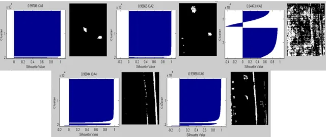
Value ... 2-63 Figure 2-17. ARES 1F Silhouette Plots with MSV and Binary Images Produced by K-

means to the Right of Each Plot... 2-64 Figure 2-18. Scree Graph of Kurtosis Values of ARES 1F Maps ... 2-66 Figure 2-19. ARES 1F Abundance Maps Sorted by KV from Koo ... 2-68 Figure 2-20. ARES 1D Abundance Maps (ICs) via FastICA Sorted by Kurtosis Value

Using Secondary Refinement ... 2-69 Figure 2-21. ARES 1D Abundance Maps (ICs) via FastICA Sorted by Kurtosis Value

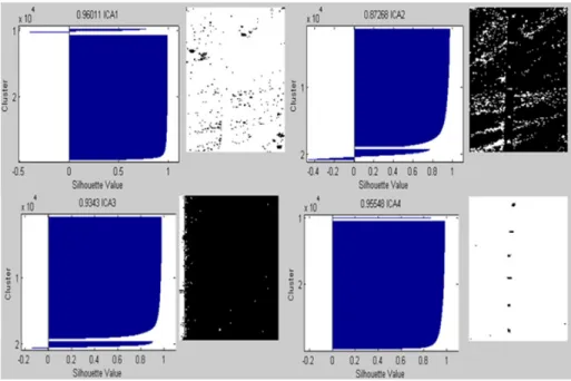
Using g = _y3_{without Secondary Refinement ... 2-71} Figure 2-22. ARES 1D Silhouette Plots with MSV and Binary Images Produced by K-

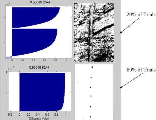
means to the Right of Each Plot... 2-72 Figure 2-23. Scree Graph of Kurtosis Values of ARES 1D Maps... 2-74 Figure 2-24. Map 4 (True Target) MSV and Binary Image Produced in 20% and 80%

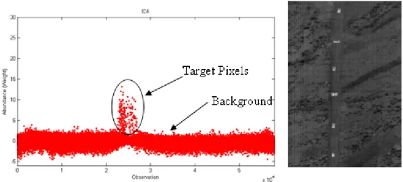
of the Trials...2-75 Figure 2-25. ARES 1D Abundance Maps Sorted by KV from Koo... 2-77 Figure 2-26. ARES 1D Abundance Row Vector Elements Corresponding to the Target

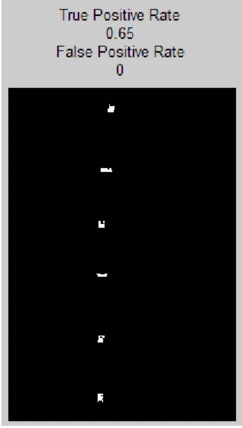
Map ... 2-80 Figure 2-27. Histogram of Scores from Map 4 of ARES 1D and Threshold ... 2-82 Figure 2-28. ARES 1D Target Detection Binary Image using Histogram Method with

Bin Width of 0.05 ... 2-83 Figure 2-29. ARES 1D Target Detection Binary Image using Histogram Method with

Bin Widths of 0.1 and 0.01 ... 2-84 Figure 2-30. ARES 1F Target Detection Binary Image using Histogram Method with

Page Figure 2-31. ARES 1F Target Thresholds for Maps 1, 2, & 3 Using

Histogram Method with Bin Widths of 0.01, 0.05, and 0.1... 2-86 Figure 3-1. Process Flow for Target Detection... 3-3 Figure 3-2. HYDICE HSI Test Images... 3-4 Figure 3-3. Truncated Version of ARES 2F ... 3-7 Figure 3-4. Finding Breakpoint between Signal and Noise Eigenvalues of White Noise

and Nonwhite Noise Using Max Euclidean Distance from Log-Scale Secant Line ... 3-10 Figure 3-5. Minimum Dimensionality Needed for ARES 1F to Isolate Targets ... 3-12 Figure 3-6. ARES 1F: Eigenvalue Curve with Max Euclidean Distance from Log Scale

Secant Line Occurring at 16th _{Eigenvalue ... 3-13}

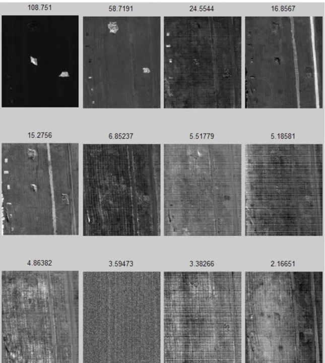
Figure 3-7. ARES 1F: Abundance Maps from 15 ICs that Result from New

Dimensionality Decision... 3-14 Figure 3-8. ARES 2F (a), ARES 1D (b), and ARES 2D (c) Dimensionality Decisions

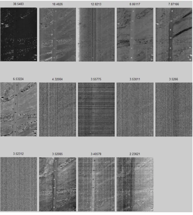
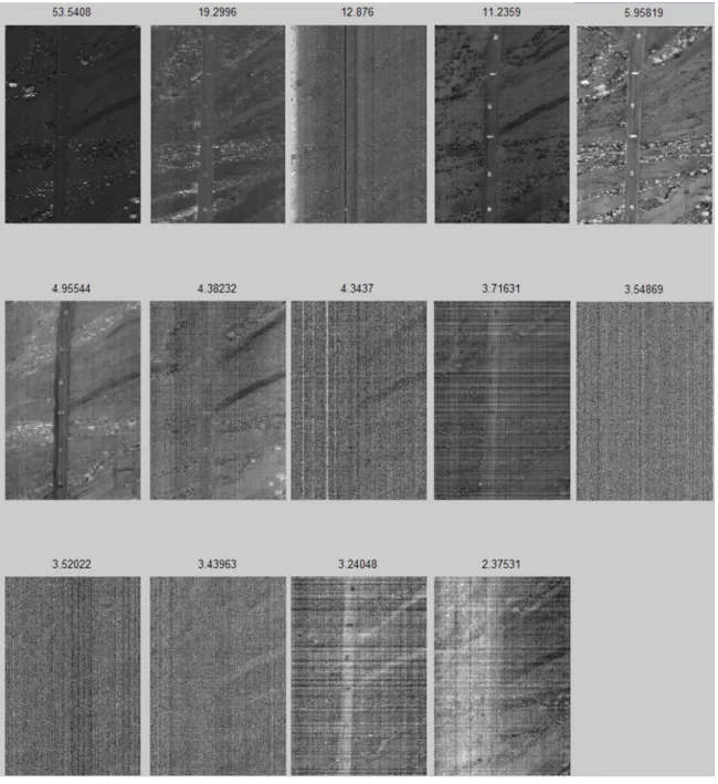
via MDSL... 3-17 Figure 3-9. ARES 2F: Abundance Maps from 15 ICs via MDSL Decision... 3-18 Figure 3-10. ARES 1D: Abundance Maps from 8 ICs via MDSL Decision ... 3-19 Figure 3-11. ARES 2D: Abundance Maps from 13 ICs via MDSL Decision... 3-20 Figure 3-12. ARES 2D: Eigenvalues of Covariance Matrix of Spectral Data with all

210 Bands... 3-21 Figure 3-13. ARES 2D: Target Identification Comparing 10 Target Maps Selected

to 8 Target Maps Selected... 3-23 Figure 3-14. ARES 1F: KV Scree Plot ... 3-30 Figure 3-15. ARES 2F: KV Scree Plot ... 3-31 Figure 3-16. ARES 1D: KV Scree Plot ... 3-32

Page Figure 3-17. ARES 2D: KV Scree Plot ... 3-33 Figure 3-18. Smallest Possible Uncertainty Region that Includes all Target Maps in

KV Feature Space ... 3-34 Figure 3-19. Image with No Targets... 3-35 Figure 3-20. ARES 1F: Independent Component Signal Plots in Order of KV with

Abundance Maps Directly Below... 3-37 Figure 3-21. ARES 1F: Map 1 Potential Target Threshold Determination... 3-39 Figure 3-22. ARES 1F: Map 4 Potential Target Threshold Determination... 3-41 Figure 3-23. ARES1F: PT SNR and Max Pixel Score for Each Signal with Potential

Target Threshold Lines ... 3-42 Figure 3-24. ARES 1F: Highest SNR and Max Pixel Score of Non-target Map... 3-43 Figure 3-25. Smallest Possible Uncertainty Region in Max Score and PT SNR

Feature Space that Includes all Target Maps ... 3-46 Figure 3-26. Group Classifications Based on Quadratic Discriminant Score with

Misclassifications Labeled... 3-48 Figure 3-27. ARES 1F: Map 3 Results after Applying Adaptive Noise Filter with

3 x 3 window size 20 times... 3-52 Figure 3-28. ARES 1D: Map 3 Results after Applying Iterative Adaptive Noise

Filter with 3 x 3 window size 20 and 100 times ... 3-53 Figure 3-29. ARES 1D: Target Identification without Iterative Adaptive Noise

Filtering... 3-54 Figure 3-30. ARES 1D: Target Identification with Iterative Adaptive Noise

Filtering... 3-55 Figure 3-31. ARES 1F: Target Identification without (left) and with (right)

Iterative Adaptive Noise Filtering ... 3-56 Figure 3-32. ARES 2F: Target Identification without (left) and with (right)

Page Figure 3-33. ARES 2D: Target Identification without (left) and with (right)

Iterative Adaptive Noise Filtering ... 3-58 Figure 3-34. AutoGAD Target Detection Algorithm ... 3-60 Figure 4-1. HSI Validation Images with Targets... 4-1 Figure 4-2. HSI Validation Images without Targets... 4-2 Figure 4-3. ARES 3F: Dimensionality Decision via MDSL ... 4-3 Figure 4-4. ARES 3F: Abundance Maps from 13 ICs via MDSL Decision... 4-4 Figure 4-5. ARES3F: PT SNR and Max Pixel Score for Each Signal with Potential

Target Threshold Lines ... 4-6 Figure 4-6. ARES 3F: Target Abundance Maps after 20 iterations of IAN Filtering .. 4-7 Figure 4-7. ARES 3F: Target Signals after IAN Filtering with Positive Signal Target

Identification Threshold... 4-8 Figure 4-8. ARES 3F: Target Signals after IAN Filtering with Positive and Negative

Signal Target Identification Threshold ... 4-9 Figure 4-9. ARES 3F: Target Identification ... 4-10 Figure 4-10. ARES 4F: Dimensionality Decision via MDSL ... 4-11 Figure 4-11. ARES 4F: Abundance Maps from 15 ICs via MDSL Decision... 4-12 Figure 4-12. ARES 4F: PT SNR and Max Pixel Score for Each Signal with Potential

Target Threshold Lines ... 4-14 Figure 4-13. ARES 4F: Target Abundance Maps after IAN Filtering ... 4-15 Figure 4-14. ARES 4F: Target Signals after IAN Filtering with Positive Signal

Target Identification Thresholds... 4-16 Figure 4-15. ARES 4F: Target Signals after IAN Filtering with Positive and

Negative Signal Target Identification Thresholds ... 4-17 Figure 4-16. ARES 4F: Target Identification ... 4-18

Page Figure 4-17. ARES 1C: Dimensionality Decision via MDSL... 4-19 Figure 4-18. ARES 1C: Abundance Maps from 8 ICs via MDSL Decision ... 4-20 Figure 4-19. ARES 1C: PT SNR and Max Pixel Score for Each Signal with

Potential Target Threshold Lines... 4-21 Figure 4-20. ARES 2C: Dimensionality Decision via MDSL... 4-22 Figure 4-21. ARES 2C: Abundance Maps from 11 ICs via MDSL Decision ... 4-23 Figure 4-22. ARES 2C: PT SNR and Max Pixel Score for Each Signal with

Potential Target Threshold Lines... 4-24 Figure 4-23. ARES 2C: False Target Abundance Maps after IAN Filtering... 4-24 Figure 4-24. ARES 2C: False Target Signals after IAN Filtering with Positive

Signal Target Identification Thresholds... 4-25 Figure 4-25. ARES 2C: Target Identification... 4-25 Figure 4-26. Max Score and PT SNR Feature Space for Test Images and

Validation Images ... 4-27 Figure 4-27. Comparison of 2-D Response to 1-D Response... 4-33 Figure 4-28. AutoGAD’s 1-D Response during Feature Selection across all Images

with Targets ... 4-35 Figure 4-29. AutoGAD’s 1-D Response across all Images without Targets... 4-37 Figure 4-30. AutoGAD’s Response in Percent TGT and TPF across Histogram Bin

Width for Target Identification (ARES 4F)... 4-39 Figure 4-31. AutoGAD’s 1-D Response during Identification across all Images with

List of Tables

Page Table 2-1. ARES 1F Summary: IC’s KV and MSV and overall Run Times ... 2-64 Table 2-2. Koo Results for ARES 1F ... 2-67 Table 2-3. ARES 1D Summary: IC’s KV and MSV and overall Run Times... 2-72 Table 2-4. Koo Results for ARES 1D... 2-76 Table 3-1. ARES 2F: Truncated Percentage of Variability Explained per Number of

Components to Retain... 3-8 Table 3-2. ARES 1F: Percentage of Variability Explained per Number of

Components to Retain... 3-8 Table 3-3. ARES 1F: 100 Runs Using FastICA Settings of pow3 vs. tanh... 3-25 Table 3-4. ARES 2F: 100 Runs Using FastICA Settings of pow3 vs. tanh... 3-26 Table 3-5. ARES 1D: 100 Runs Using FastICA Settings of pow3 vs. tanh... 3-27 Table 3-6. ARES 2D: 100 Runs Using FastICA Settings of pow3 vs. tanh... .3-28 Table 3-7. ARES 1F: New Target Feature Filters Summary 100 Reps Target Maps Highlighted in Gray ... 3-44 Table 3-8. ARES 2F: New Target Feature Filters Summary 100 Reps Target Maps Highlighted in Gray ... 3-44 Table 3-9. ARES 1D: New Target Feature Filters Summary 100 Reps Target Maps Highlighted in Gray ... 3-45 Table 3-10. ARES 2D: New Target Feature Filters Summary 100 Reps Target Maps Highlighted in Gray ... 3-45 Table 3-11. AutoGAD Algorithm Results for Test Images (100 Reps) ... 3-61 Table 3-12. Test Image Statistics... 3-61 Table 4-1. AutoGAD Results for Validation Images (100 Reps)... 4-28

Page Table 4-2. Validation Image Statistics ... 4-29 Table 4-3. Comparison of Mean and Variance of Euclidean Distance from Ideal Point without and with IAN Filtering on the Range from 0.045-0.064 ... 4-42

IMPROVED FEATURE EXTRACTION, FEATURE SELECTION, AND IDENTIFICATION TECHNIQUES THAT CREATE A FAST UNSUPERVISED

HYPERSPECTRAL TARGET DETECTION ALGORITHM

I. Introduction 1.1 Background

Distinguishing man-made objects from natural objects in rural environments is of particular interest when man-made objects are targets within the military context.

Hyperspectral sensors offer a passive means (as opposed to radar where an enemy can be alerted to surveillance) by which to identify targets by exploiting information within the electromagnetic spectrum (EM). The typical range of the EM spectrum exploited is the optical range which includes ultraviolet, visible, and infrared wavelengths as shown in Figure 1-1 below. Optical regions useful for remote sensing extend beyond the regions where photography can be used (Landgrebe, 2003: 13).

The specific physics and hardware specifications to collect hyperspectral images (HSI) is beyond the scope of this thesis, but a general explanation of the nature of an HSI image will be explained.

A particular area being imaged by an HSI sensor is divided into a raster grid with each grid cell or pixel corresponding to a rectangular sub-region of the image. The physical dimensions of the pixel correspond to the spatial resolution of the sensor which could range typically from some fraction of a meter to tens of meters (Smetek, 2007:16). Other than spatial resolution, the sensor can be characterized by the range of EM

wavelengths it is capable of measuring and the smallest detectable wavelength difference (spectral resolution). Hyperspectral sensors typically record energy, measured in

radiance (watts per square meter per steradian), over hundreds of discrete intervals called spectral bands (the width of the interval is determined by the spectral resolution) across some subset of the optical wavelengths. The sensor records the amount of energy radiated by each pixel over all the sensor’s spectral bands.

It may not be possible to distinguish between natural foliage and camouflage netting concealing tanks or troop tents when examining a normal RGB (red green blue) digital image taken from a surveillance aircraft. However, when analyzing the same image taken with an HSI sensor that considers more than just the visible spectrum, the camouflage material will reflect electromagnetic energy different than the surrounding foliage and thus can be identified. This difference in the radiated energy can be observed when analyzing the spectral signatures of the objects. The spectral signature of a pixel would be a plot of the pixel’s response across each of sensor’s spectral bands.

It should be noted that whereas the HSI sensor collects data in units of radiance for each spectral band, data is usually converted to reflectance. When atmospheric correction is performed on the radiance data, the effects of path radiance (energy reflected by the atmosphere into the sensor that does not reach the ground) and skylight (energy that bounces off the atmosphere and is reflected by the ground) are removed. The resulting data is in terms of reflectance signatures and represent the relative amount of energy from the sun (without path radiance and skylight) that hits the Earth’s surface and is reflected (Smetek, 2007: 12-13).

1.2 HSI Data Representation

Before proceeding further, the reader should be acquainted with how HSI data is organized for processing. HSI data is represented as a cube where the first two indices of

(

i j k, ,

)

coordinate triple represent the spatial location of the pixel in the image and the third index defines the pixel’s reflectance response in the_kth_{spectral band. Figure 1-2} below is an example of an image cube.

Figure 1-2. Hyperspectral Data Cube (Shaw and Manolakis, 2003: 13)

i

k

j

i

k

j

In order to perform operations on the data cube such as mean and covariance calculations for example, the data cube is reshaped in to a data matrix. Say this particular image was 150 pixels by 200 pixels by 210 bands making a total of 30,000 pixels. Reshaping this cube into a data matrix would result in a matrix with dimensions of 30,000 pixels by 210 bands. Figure 1-3 shows the process.

Figure 1-3. Reshaping Image Cube into Data Matrix

As shown in Figure 1-3 each pixel in the image cube can be considered a vector where each element is a reflectance response in each of the k spectral bands. Starting from the top left of the cube and moving down the first column

(

j=1

)

of the image, each pixel vector in the first column is formed into a column in the data matrix. The process is

Each pixel vector is a column in the data matrix with i j ni = columns 11 12 1 21 22 2 1 2

...

...

.

.

.

n n k k kn

x

x

x

x

x

x

x

x

x

⎡

⎤

⎢

⎥

⎢

⎥

⎢

⎥

⎢

⎥

⎣

⎦

1 x 2 x k x 1 2

.

k

x

x

x

x

⎛ ⎞

⎜ ⎟

⎜ ⎟

=

⎜ ⎟

⎜ ⎟

⎝ ⎠

Pixel Vector Image Cube k n

Each pixel vector is a column in the data matrix with i j ni = columns 11 12 1 21 22 2 1 2

...

...

.

.

.

n n k k kn

x

x

x

x

x

x

x

x

x

⎡

⎤

⎢

⎥

⎢

⎥

⎢

⎥

⎢

⎥

⎣

⎦

1 x 2 x k x 1 2

.

k

x

x

x

x

⎛ ⎞

⎜ ⎟

⎜ ⎟

=

⎜ ⎟

⎜ ⎟

⎝ ⎠

Pixel Vector Image Cube k n

Each pixel vector is a column in the data matrix with i j ni = columns 11 12 1 21 22 2 1 2

...

...

.

.

.

n n k k kn

x

x

x

x

x

x

x

x

x

⎡

⎤

⎢

⎥

⎢

⎥

⎢

⎥

⎢

⎥

⎣

⎦

1 x 2 x k x 1 x 2 x k x 1 2

.

k

x

x

x

x

⎛ ⎞

⎜ ⎟

⎜ ⎟

=

⎜ ⎟

⎜ ⎟

⎝ ⎠

Pixel Vector Image Cube k n

repeated starting with the second column and finishing with the _j th _{column. The result is} a data matrix with k rows (one for each spectral band) and n columns (one for each pixel observation). It should be noted that in some texts the data matrix is transposed from the one presented in Figure 1-3 to be n pixel observationsby k spectral bands.

1.3 Approaches

In order to find targets two main methods are pursued. The first method is

referred to as signature matching. Here, one compares pixel vectors (i.e. pixel signatures) to a library of target reflectance signatures to determine which pixels belong to targets of interest. Figure 1-4 below shows how spectral signatures of different materials may differ across the spectral bands of an HSI sensor.

The second method is referred to as anomaly detection. Although definitely not comprehensive, two common categories are (i) distribution based anomaly detectors (local or global) that assume a distribution (typically normal) of the pixel vectors and (ii) global linear mixture model detectors.

Distribution Based Anomaly Detectors

In local anomaly detection, a scanning window (which is some fraction of the size of the entire image) is moved over the image and centered on a pixel of interest. At each stop the local mean and covariance is calculated and if the centered pixel of interest is beyond some statistical distance threshold (typically a Mahalanobis distance) from the mean then it is nominated as an outlier. Such local anomaly detectors are referred to as local normal models, i.e. the pixel vectors are assumed to be distributed Gaussian (normal) with meanμ and covariance Σ. The RX detector is one such detector.

According to Stein, Beaven, Hoff, Winter, Schaum, and Stocker (2002:62), the local Gaussian model may not be a valid for hyperspectral data if relatively small regions contain multiple materials. Based on goodness-of-fit tests of a hyperspectral scene to a local normal model, the local normal model was rejected for more than 90% of the pixels. Thus, the local normal model may not capture the complexity of hyperspectral imagery. They assert that global mixture distributions will provide more accurate descriptions.

Global normal mixture models assume an image is made of C classes where each class has a separate multivariate Gaussian (normal) distribution with parametersμ_cand

c

Σ for class c. The overall pdf of the scene is described by a Gaussian mixture distribution:

( )

(

)

c 1 1 , ; 0; 1 C C c c c c c c g x π N x u π π = = =

∑

Σ ≥

∑

= (1.1) where π_c is the probability of belonging to class c (Stein and others, 2002:63). Stein et al. use a stochastic expectation maximization (SEM) method to determine the location of the classes and their parameters. However, as Smetek points out, no guidance is given on how to determine the number of classes C (Smetek, 2007:48). Rather than the SEM approach, another way to determine the location of the classes is via the k-means clustering algorithm. However, the number of classes k is subjectively specified by the user (Smetek, 2007:49). Similar to the local anomaly detectors that identify anomalous pixels as statistical outliers in the local scanning window, the Gaussian mixture models identify anomalous pixels that are outliers for each of these clusters’ distributions.

Global Linear Mixture Model Detectors

Rather than presuming some distribution of the pixel vectors in the scene, this approach assumes that each pixel vector observation is a convex combination of a deterministic number of endmembers, i.e. a finite number of distinct spectral signatures. The coefficients of the convex combination are interpreted as the fractional abundance of each endmember in a particular pixel. As will be explained in great detail in chapter 2, one must solve for the abundances in what is called unmixing the image. Target-like endmembers are identified based on properties of the abundance estimates (Stein and others, 2002:60). Given this research will employ the linear mixture model of HSI, a lengthy discussion of this model and a solution methodology to solve for the abundances via a technique called independent component analysis (ICA) will be presented in chapter 2.

1.4 Research Objectives

Based on the linear mixture model of HSI, this research seeks to develop a fast and truly autonomous (unsupervised) global anomaly detector, dubbed AutoGAD, to locate targets in an HSI image. Autonomous, implies the only input from the user is the image cube. The rest of the decisions to identify targets are made via the AutoGAD algorithm. By fast, the goal is to be able to process images in terms of minutes and even seconds in order to provide real-time targeting for operational employment.

As will be discussed in chapter 2 and chapter 3, feature extraction refers to reducing the dimensionality of HSI data by projecting the k dimensional data onto a lower dimensional orthogonal subspace (commonly via a technique referred to as principal components analysis) where much of the structure of the original data is maintained. The first objective of this thesis is to develop a way to effectively,

efficiently, and autonomously determine the number of dimensions to project the data. As will be explained later, the correct number of dimensions to choose, refers to the number of distinct endmember signatures present in the image.

After reducing the dimensionality, the features (which correspond to the n pixels’ scores on each of the new coordinate axes) will be projected again to a new set of axes that are not only orthogonal, but independent via a method previously mentioned called ICA. This projection is determined by an optimization scheme which will be rigorously developed in chapter 2. The second objective of this thesis will be to determine which objective function, that approximates a measure of independence, yields the least amount

of variability in the solution per each test image it is applied to. This will ensure a level of robustness to the new detector.

From the final set of features produced by ICA, a process called feature selection must choose which features are target like based on some statistical measure of target ‘likeness’. Currently, features with high kurtosis values are used to nominate features that belong to the target class. However, the process of selecting the cutoff kurtosis value between target classes and non-target classes is a supervised procedure. As will be illustrated in chapter 3, attempts to automate the procedure is problematic and the overlap between non-target kurtosis values and target kurtosis values calls for the investigation of alternate measures of target ‘likeness’ that minimizes the overlap between the classes so that the cutoff decision between the classes can be automated. This is the third objective of this thesis.

As previously explained a feature is an n dimensional vector which represents each of the n pixels’ scores on a particular axis in the ICA space. The selected target features, are in other words the selected target axes in the ICA space. The next step in the target detection process is to identify which pixels in each of the selected features are the target pixels. The fourth objective of this thesis is to find an unsupervised way to locate these pixels that reduce the amount of false positives detected.

1.5 Assumptions

Anomaly detectors, since they do not assume a priori knowledge of target

signatures, must make a few assumptions about the nature of targets. Further the domain of effective application of anomaly detectors is limited. Targets in an image are assumed

to be a small, rare occurring class (as opposed to a large class like a forest) and have a spectral signature distinct from the rest of the spectral signatures present in the image. Man-made objects in large rural areas of large classes of natural occurring objects like dirt, grass, trees, bushes, gravel, sand, etc...meet the definition of targets. However, in an urban environment, most of the objects are man-made objects. Thus, the definition of small, rare occurring class and distinct spectral signature breaks down. For this reason the domain of the new anomaly detector is assumed to be rural environments.

Although not mentioned previously, an important initial processing requirement before executing AutoGAD is the removal of what are called the atmospheric absorption bands from the data. Atmospheric absorption bands are bands in which the energy at these wavelengths is almost entirely absorbed by the atmosphere. Therefore, the sensor detects primarily random noise at these wavelengths. Given the wavelengths of

atmospheric absorption are known, the bands in the sensor referred to as the noise bands are assumed to be known. Further, in addition to the atmospheric absorption bands there may be other bands in the sensor that record significant noise, often at the extremes of the sensor’s band range (Taitano, 2007:33-34). Before the application of the AutoGAD, it is assumed that the user has a priori knowledge of the ‘good’ non-noise bands in the sensor. For each different sensor that employs AutoGAD a separate input for the good bands will be required.

Finally, the set of test and validation images presented in chapters 3 and 4 are assumed to be a representative sample from the domain of rural HSI images with targets.

II. Literature Review and Critical Analysis of Current Practices 2.1 Linear Mixture Model (LMM) for HSI

As previously described, the LMM assumes each pixel vector is a “linear mixture of a discrete number of pure deterministic material spectra” (Chang, 2007:108).

Terminology such as ‘pure spectra’, ‘pure materials’, or ‘pure pixels’ are often referred to as endmembers each having a characteristic spectral signature.

The physical basis for the linear mixture model is that hyperspectral image measurements often capture multiple material types in an individual pixel and that measured spectra can be described as a linear superposition of the spectra of the pure materials from which the pixel is composed. The weights of the superposition correspond to the relative abundances of the various pure materials. This assumption of linear superposition is

physically well-founded in situations, for example, where the sensor response is linear, the illumination across the scene is uniform, and there is no scattering (Chang, 2007:108).

Nonlinear mixing occurs when, for example, there is multiple scattering of light between elements in a scene.

Despite the potential for nonlinear mixing in real imagery, the linear mixing model has been found to be a fair representation of hyperspectral data in many situations (Chang, 2007:108).

The LMM for a particular pixel observation i, where i = 1,2,…,N observations, formulates as follows:

1 11 12 1 1 2 21 22 2 2 1 2 1 2 1 2 ... . . . . . j P j j P j j j Pj Kj K K KP Kj j j P x r x r s s s x r x r ε ε ε ε ε ε ε ε ε ε ε ε ⎛ ⎞ ⎛ ⎞ ⎛ ⎞ ⎛ ⎞ ⎛ ⎞ ⎜ ⎟ ⎜ ⎟ ⎜ ⎟ ⎜ ⎟ ⎜ ⎟ ⎜ ⎟₌ ⎜ ⎟₊ ⎜ ⎟_{+ +} ⎜ ⎟₊⎜ ⎟ ⎜ ⎟ ⎜ ⎟ ⎜ ⎟ ⎜ ⎟ ⎜ ⎟ ⎜ ⎟ ⎜ ⎟ ⎜ ⎟ ⎜ ⎟ ⎜ ⎟ ⎜ ⎟ _{⎝ ⎠ ⎝ ⎠ ⎝ ⎠} ⎜ ⎟ ⎝ ⎠ ⎝ ⎠ 1 P j j pj p p j j KxP j or x s r x E s r ε = = + = ⋅ +

∑

(2.1) where j

x ≡pixel column vector where each element is an intensity value (in terms of spectral reflectance) for one of K spectral bands for observation j, where j=1,..., .N

p

ε ≡column vector of E_KxPthat represents the spectral signature for the th

p endmember, where p=1, 2,..., .P Each element is an intensity value for one of the K spectral bands.

pj

s ≡abundance fractions of the _pth_{endmember in} j

x , the _jth _{pixel vector} observation. Note, since s_pj are abundance fractions,

1 1 for 1,..., P pj p s j n = = =

∑

and s_pj ≥0 for p=1,..., and P j=1,...,N j

r ≡random vector representing additive Gaussian sensor noise with a mean of zero for the _jth_{pixel vector observation}

Note that in the case where a single pixel vector,x_j, is an actual endmember, i.e. pure pixel, spjwould be zero for all p except for the endmember occupying that particular

observation. Further, note the sum-to-one and non-negativity constraints on the abundance fractions.

Because of the random nature of r, each measured x should be considered a realization of a random vector process. It may also be appropriate to consider the abundance fractions as a random component, but an inherent assumption in the LMM is that the endmember spectra,εP, are deterministic (Chang, 2007:110).

If (2.1) is expressed in terms of an entire data matrix, X, where each column is a distinct observation of a pixel vector, one has:

11 12 1 11 12 1 11 12 1 21 22 21 22 21 22 1 2 1 2 1 2 1 2 1 2 ... ... ... . . . . . . . ... ... ... N P N KxN K K KN K K KP P P PN N x x x s s s x x s s R x x x s s s x x x ε ε ε ε ε ε ε ε ε ε ⎛ ⎞ ⎛ ⎞ ⎛ ⎞ ⎜ ⎟ ⎜ ⎟ ⎜ ⎟ ⎜ ⎟₌⎜ ⎟_⋅⎜ ⎟₊ ⎜ ⎟ ⎜ ⎟ ⎜ ⎟ ⎜ ⎟ ⎜ ⎟ ⎜ ⎟ ⎝ ⎠ ⎝ ⎠ ⎝ ⎠ P KxN KxP PxN KxN or X E S R ε = ⋅ + (2.2)

Notice that the elements of the _jth_{column of} PxN

S , represent the separate fractional abundances of the P endmembers signatures ,

ε ε

₁

, ,...,

₂

ε

_P (column vectors of E), in observation j. Furthermore, the elements of _pth_{row of}

PxN

S , represent the abundance fractions of a single endmember,

ε

_p, in each of N observations. Thus, if one where to plot the values of the _pth _{row of}

PxN

S (which is termed an abundance map) and the signal shows ‘high’ abundance values for observations, say observation 25 through 35, as

compared to the values for the other observations, then one could conclude that those

pixel observations have a high concentration of the _pth_{endmember. Each abundance row} vector can be considered a feature in the image.

Another important fact to consider for the LMM is that the model is an additive only model. Given thatE_KxP is matrix of endmember signatures where each element is a reflectance value (nonnegative) in a particular spectral band and the abundance matrix,

PxN

S , contains nonnegative fractions, the LMM is a purely additive model (allowing no subtractions).

2.1.1 Abundance Maps and Target Detection

A Priori Knowledge of Endmember Matrix

If the endmember matrix E (i.e. total number of endmembers in the image and their respective spectral signatures) is known a priori then the problem is to solve for the abundance matrix,S_PxN, to unmix the hyperspectral image. The abundance matrix is generally solved using constrained least squares methods. The estimated abundance matrix row vectors recovered are usually formed into images and are termed the

abundance maps, as described earlier, for each respective endmember (Chang, 2007:111). The abundance matrix row vector is simply reshaped into the original image pixel length by width and plotted on a grey scale (scaled between 0 and 1) to create an abundance map. Analysis of these abundance maps is the key to identifying targets of interest. Pixels with high abundance values in abundance map p corresponding to endmember p

(which is a signature of a particular target of interest or desirable endmember) identify the location of that particular target. Figure 2-1 is an example of such an abundance map.

Figure 2-1. Abundance Map for Tank Endmember

No A Priori Knowledge of Endmember Matrix

Signature Matching

Of course, if one has no a priori knowledge of the endmember matrix, the problem of solving for the endmember matrix and abundance matrix (termed unmixing) in hyperspectral images is much harder. One must determine both the endmember matrix and the abundance matrix from knowledge of just the observed matrix X. Such a problem falls into the category of a much more general problem referred to as blind source

separation (BSS). The term blind indicates that little or no information is available on either of the matrices that multiply to form the observed matrix X (Varshney and Arora, 2004:110). Two particular solutions applied to the problem of BSS, independent

component analysis (ICA) and nonnegative matrix factorization can be used to solve for both matrices. One particular target identification algorithm, ICA-EEA

(ICA-Endmember Extraction Algorithm), performs the ICA algorithm to solve the BSS

problem, unmixing the hyperspectral data set. Target candidate pixels are identified from each abundance map by choosing the pixel with the highest absolute abundance value from each map. These pixels are hypothesized to represent pure endmembers. The signatures of these pure endmembers, which are obtained from the corresponding pixel vectors from the original unmixed data matrix, X, are compared to the material signatures of targets of interest to identify which abundance maps may contain those targets of interest (Wang and Chang, 2006:623314-3).

Anomaly Detection

In the area of anomaly detection, one does not even know the signatures of the targets of interest and wishes to identify targets in terms of just anomalous occurrences in the overall image. The hypothesis is that target materials are relatively rare, producing abundance maps with relatively few intense pixels (Smetek, 2007:46). Abundance maps corresponding to these target materials will have a relatively constant dark background (representing very low values of abundance) with the few target pixels highlighted brightly (representing high abundance values). Such an abundance map represents a scenario with small objects and a large homogeneous background. In such a map, if one were to take the kurtosis value of the abundance vector that was used to form the map, the value would be high compared to an abundance map representing a large class, like for example a large sections of trees. Thus, one could select the maps with the highest kurtosis as the one containing information about small objects. Robila and Varshney make a determination of the number of maps to retain based on a scree graph of the kurtosis values. They state that a considerable slope change represents the border

between one class of maps, in our case target classes, to another, non-target classes (Robila and Varshney, 2002:177). An example of this small class (i.e. target) feature selection via the scree graph of kurtosis values will be presented later in this chapter in section 2.4. Once the frames with the highest kurtosis are selected, those pixels with abundance values higher than a determined threshold will be classified as targets in the target identification phase.

2.1.2 Dimensionality Reduction (Feature Extraction)

Spectral unmixing is usually performed within a subspace of the original K spectral bands. It has been proven that high-dimensional space is mostly empty, and multivariate data are usually in a lower dimensional structure. As a result, for any particular hyperspectral image, this K-dimensional data can be projected to a lower dimensional subspace without losing significant information and class separability

(Landgrebe, 2003:270). This process is referred to as feature extraction. The features are the new variables that define the dimensions of the subspace. The focus is to increase the separation between classes within each feature (i.e. find projections where the new variables are uncorrelated) while reducing overall noise (Robila and Maciack, 2006:2). Further, since the number of endmembers, P, is not known, the dimension of the

subspace is considered to be the number of distinct endmembers for the given image (Change, 2007:112). Determination of the number of endmembers via a dimensionality reduction technique called principal components analysis will be discussed next.

2.1.3 Principal Components Analysis (PCA)

PCA linearly transforms data into a subspace where the new variables

(components) are decorrelated and ranked in decreasing order of variance. Consider a

random hyperspectral pixel vector, xT =

(

x₁,...,x_K

)

in K spectral bands. To find the first principal component, one must find a projection of this vector

( )1 _{( )1} 11 1 21 2 ... 1 T

K K

y =g x g x= +g x + +g x (2.3) such that the variance of the projection, cov

( )

y_{( )1} , is maximized subject to the

projection, _{( )} 1

g , being of unit norm.

( )

( )

( ) ( ) ( )

(

)

( ) ( ) 1 1 1 1 1 1 MAX

cov note: =cov( )

g s.t. 1 T T x x T g x g g x g g = ∑ ∑ = (2.4)

If ∑_xpositive definite, then to find _{( )} 1

g one must satisfy only the necessary condition, where the gradient of the Lagrangian is zero. The Lagrangian of (2.4) and gradient of the Lagrangian will be ( ) ( )

(

1, 1

)

( )1 ( )1 ( )1

(

( ) ( )1 1 1

)

T T x L g λ =g ∑ g −λ g g − (2.5) ( ) ( ) ( ) ( ) ( ) 1 1 1 1 1 2 2 ₀ 0 1 x T g g L g g λ Σ − ⎛ _{⎞ ⎛ ⎞} ⎜ ⎟ ∇ = _{= ⎜ ⎟} ⎜ ₋ ⎟ _{⎝ ⎠} ⎝ ⎠ (2.6) Note that ( )₁ ( ) ( )1 ₁

(

( )1

)

( )₁ 2Σ_xg −2λ g = ⇒ Σ −0 _x λ I g =0 (2.7) In order to have a solution for _{( )}

1

( )1 0 x λ I

∑ − = (2.8)

Thus, the solution,λ_{( )1} , for (2.8) is the largest eigenvalue of ∑_xwhich means g_{( )1} is the normalized eigenvector associated withλ_{( )1} . The second principal component

( )2 ( )₂ 12 1 22 2 ... 2 T

K K

y =g x g x= +g x + +g x (2.9) is found by solving (2.4) with the additional constraint, _{( ) ( )}

1 2 0

T

g g = . Using the same argument above it can be shown that _{( )}

2

g is the normalized eigenvector associated with the second largest eigenvalue of∑_x, λ_{( )2} . The process is repeated until all K normalized eigenvectors of ∑_xare found where each eigenvector is orthogonal to every other

eigenvector (Dillon and Goldstein, 1984:28). Now by definition of eigenvalues:

( ) ( ) ( ) ( ) ( ) ( ) ( ) ( ) ( ) 1 1 1 2 2 2 x x x _K K _K g g g g g g λ λ λ Σ = Σ = Σ = ⇒ _{( ) ( ) ( ) ( ) ( ) ( ) ( )1 2 ( ) ( )} 1 2 ... 1 2 ... xg xg xg _K λ g λ g λK g _K ⎡_{Σ Σ Σ} ⎤ ⎡₌ ⎤ ⎢ ⎥ ⎢ ⎥ ⎣ ⎦ ⎣ ⎦ ⇒Σ_x⎣⎢⎡g_{( )1} g_{( )2} ... g_{( )K ⎦ ⎣⎥ ⎢}⎤ ⎡= g_{( )1} g_{( )2} ... g_{( )K} ⎤_⎦⎥D, where ( ) ( ) 1 . . K D λ λ ⎛ ⎞ ⎜ ⎟ ⎜ ⎟ = ⎜ ⎟ ⎜ ⎟ ⎜ ⎟ ⎝ ⎠ ⇒Σ ⋅ = ⋅_x G G D (2.10) Because G is a matrix of unit norm eigenvectors of a covariance matrix, G isorthonormal and _{G G I}T_{⋅ = . Thus, left multiplying (2.10) by G ,} T _{one has the result:}

T x

G ⋅Σ ⋅ =G D (2.11) (2.11) is significant because the goal is to have new variables,

(

y₍₁₎,y₍₂₎,...,y_{( )K}

)

=y', that are uncorrelated. Notice

( )

( )

cov cov T T

x

y = G x =G ⋅Σ ⋅ =G D (2.12) Since D is a diagonal matrix the new variables (components) are uncorrelated with

thevar

( )

y_{( )i} =λ_i, for i=1,...,K.

Now to address the issue of dimensionality reduction, the goal is to retain enough of the y_{( )i} 'sso that amount of variability explained is enough to preserve the significant information and class separability as was explained previously in the citation from Landgrebe. The total variance of the hyperspectral image can be defined:

Total Variance ≡ trace

( )

Σ_x = 2 1 K ii i σ =

∑

(2.13) Right multiplying (2.10) by G’ T x G D G Σ = ⋅ ⋅ (2.14) So 2 1 K ii i σ =

∑

= trace (Σ_x) = trace

(

_{G D G⋅ ⋅} T

)

_{= trace}

(

_{G G D}T_{⋅ ⋅}

)

_{= trace}

( )

_{D =} 1 K i i λ =

∑

(2.15) Thus, Total Variance ≡ 1 K i i λ =

∑

(2.16)

Thus, (2.13) and (2.16) give the important result that the total variance of the original variables is equal to the sum of the variances for all K principal components (Dillon and Goldstein, 1984:29).

Determining Dimensionality

One way to determine what the reduced dimensionality of the image is to

calculate a selected subset of components’ percentage of variance explained. An analysis of their corresponding eigenvalues yields:

1 1 P i i K i i

λ

λ

= =

∑

∑

= % of variance explained by selected subspace (2.17)

Robila and Varshney choose 99.9% in their cited research.

Another way to determine the dimensionality of the subspace comes from the assertion that covariance of the random hyperspectral pixel vector is made of the true signal covariance and noise. The true signal covariance is contributed by the true number, P, of distinct endmember signatures in the image. Beyond the _Pth_eigenvalue of∑_x, the eigenvalue distribution becomes constant with the value of the constant

eigenvalues equal to the covariance of the noise term, r in (2.1), _σ2_{I, i.e. white noise} (Chang, 2007:112; Hyvärinen and others, 2001:131). As reproduced from Stocker et al., Figure 2-2 (a) shows a plot of eigenvalues from simulated data with 64 bands and 8 signals, i.e. a true dimensionality of 8, with added white noise of variance 1. Notice the constant floor at 1, _σ2_{, in Figure 2-2 (a). However in Figure 2-2 (b), due to finite-sample} estimation errors, instead of a constant eigenvalue noise floor at_σ2_{, one can view a ‘tilted}

ramp’ in the general vicinity of _σ2_{. The distribution of the noise eigenvalues follow} approximately an asymptotic distribution called Silverstein’s distribution, provided the eigenvalues are from a white noise covariance matrix formed from independently

identically distributed noise vectors (Stocker and others, 2003: 654). If the covariance of

the noise term, r, is not white, i.e.

( )

2 2 2

1 2

cov r =⎡_⎣σ σ, ,...,σ_K⎤_⎦⋅I, as depicted in Figure 2-2 (b), this nonwhite sensor noise added to the same signals imparts additional tilt into the sample eigenvalue curve (Stocker and others, 2003: 652). Fitting the white noise eigenvalues to the Silverstein distribution approximately locates the ‘knee’ in the eigenvalue curve that separates the signal and noise eigenvalues as shown in Figure 2-2 (c). However, for many hyperspectral sensors, noise is not white across the spectral range of the instrument, and no analogous closed form expression for the asymptotic eigenvalue density exists in the nonwhite noise case (Stocker and others, 2003: 657). Thus, locating the ‘knee’ is a more difficult problem due to the absence of a closed form theoretical distribution and requires some estimation of the distribution of the nonwhite noise eigenvalues. This is accomplished via an estimate of the spectrally varying noise

level 2 2 2

1, 2,..., K

σ σ σ

⎡ ⎤

⎣ ⎦ extracted from scene data. Stocker et al. provide a parametric

in-scene approximation to the spectral nonwhite noise characteristic to approximate

2 2 2

1, 2,..., K

σ σ σ

⎡ ⎤

⎣ ⎦ (Stocker and others, 2003: 657-664).

By locating the breakpoint in the eigenvalue curve between signal and noise of the covariance matrix of the data, and discarding those eigenvectors associated with the eigenvalues corresponding to noise, one can improve the signal to noise ratio of the data in the PCA space.

Figure 2-2. (a) True eigenvalues, (b) sample eigenvalues, and (c) Silverstein model fit for simulated 64-band data with 8 signal modes

and additive sensor noise (Stocker and others, 2003: 653, 657)

(a)

(b)

(c)

Thus, after some decision is made on the number principal components to retain denoted by P, our original K-dimensional hyperspectral image is projected onto a P -dimensional orthogonal subspace by a linear transformation matrix defined by selecting the P eigenvectors (where P represents the number of retained eigenvectors) associated with the P eigenvalues in (2.17) and discarding the rest of the eigenvectors. This matrix of retained eigenvectors is applied to X shown in (2.18) below,

11 12 1 11 12 1 21 22 21 22 1 2 1 2 ... ... . . . . . . . . . . ... ... N K PxN K K KN P P PK T PxK KxN x x x g g g x x g g Y x x x g g g G X ⎛ ⎞ ⎛ ⎞ ⎜ ⎟ ⎜ ⎟ ⎜ ⎟ ⎜ ⎟ = ⎜ ⎟ ⎜ ⎟ ⎜ ⎟ ⎜ ⎟ ⎝ ⎠ ⎝ ⎠ i (2.18)

where the th row of T represents the th retained eigenvector of x

p G p Σ .

Recall the LMM presented in (2.2). After finding the lower dimensional subspace, the new form of the LMM model is

11 12 1 11 12 1 11 12 1 21 22 21 22 21 22 1 2 _{1 2 1 2} ' ' ' ' ' ' ' ' ' ' ' ' ' ' ' ' ' ... ... ... . . . . . . . ... _{... ...} N P N PxN P P PN _{P P PP P P PN} s s s y y y y y s s R y y y _{s s s} ε ε ε ε ε ε ε ε ⎛ ⎞ ⎛ ⎞ ⎛ ⎞ _{⎜ ⎟ ⎜ ⎟} ⎜ ⎟ _{⎜ ⎟ ⎜ ⎟} ⎜ _{⎟ =⎜ ⎟⋅⎜ ⎟+} ⎜ ⎟ _{⎜ ⎟ ⎜ ⎟} ⎜ ⎟ _{⎜ ⎟ ⎜ ⎟} ⎝ _{⎠ ⎝ ⎠ ⎝ ⎠} ' ' ' _{PxN PxP PxN PxN} or Y =E ⋅S +R (2.19)

Notice the endmember matrix in (2.19) to be determined is now a square matrix which is advantageous when employing methods to solve for the endmember matrix and

abundance matrix simultaneously. It is important to note that, whereas the _jth_{column of} X represented the _jth_{pixel’s signature across the K spectral bands, the j}th_{column of Y in}

(2.19) represents the _jth_{pixel’s signature across the P principal components. Thus, when} solving for the endmember matrix in (2.19), the columns of this new square endmember

matrix denoted by E'instead of E represent the signatures of the endmembers in the principal component space not signatures of the endmembers in terms of reflectance of the original K spectral bands. Thus, one loses the physical interpretability of the solved endmember matrix in this new space. Further, given that the principal component space

is not nonnegative as is the case in the spectral reflectance space, the Y matrix and theE'

matrix will have negative terms in (2.19) and thus no longer strictly conforms to the additive only LMM in (2.1) since subtractions will occur. However, based on this author’s review of the myriad of literature available on dimensionality reduction of hyperspectral images, PCA is the most common tool used to effectively reduce the dimensionality of a hyperspectral image. Another approach called nonnegative PCA is suggested by several sources as a reduction technique that produces nonnegative components. This technique should be investigated and compared to PCA to see if the additional nonnegative restriction outperforms target detection algorithms using

traditional PCA image compression as a preprocessing technique. However, this thesis due to its limited scope will employ traditional PCA.

2.1.4Limitations of the LMM

Recall that a basic assumption in the LMM is that the endmembers are

deterministic, i.e. within an endmember, the signature has no variability. Further, the assertion is that the mixtures of a small number of deterministic spectra (endmembers)

can be used to represent all of the non-noise variance in a hyperspectral image. However, there is natural signature variation to almost all materials that would be selected as

endmembers in a hyperspectral image. Also, practically, there is a limit to how many endmembers can be used to represent a scene. Thus, any particular endmember may not necessarily represent just one material but a class of materials that are spectrally similar. Thus, the spectral signature of the endmember will have variation. Further, another source of endmember variation is illumination. A particular endmember in shade will have a different signature than the same endmember exposed to direct sunlight. Thus, the endmembers are not truly deterministic signature vectors, but random vectors. However, when the within endmember variance is small compared to the between endmember variance, the deterministic endmember assumption may remain relatively valid. The other assumption of linearity of the mixing fails if

there is significant three-dimensional structure within a given pixel and where the optical energy makes multiple bounces between objects before exiting in the direction of the sensor (Chang, 2007:27).

However, if the mixing scale at each pixel is macroscopic, the linear model holds (Chang, 2007:149). Next, a solution to the LMM called independent component analysis will be presented followed by a discussion of how it approximately fits into the LMM of HSI. When discussing independent component analysis it is assumed we are still operating in the reduced PCA space.

2.2 Independent Component Analysis (ICA)

Independent Component Analysis (ICA) introduced in the early 1980’s is a multivariate data analysis method where, given a linear mixture of statistically

independent components, these components are recovered by solving for an unmixing matrix (Varshney and Arora, 2004:109). Whereas PCA finds the transform of the observed data that decorrelates the observed variables through the use of second-order statistics (i.e. a transform based on the eigenvectors of the covariance matrix), ICA utilizes higher-order statistics to find projections of the data where the components are independent, a stronger statement than uncorrelated. Throughout the past two decades from the initial development the ICA technique in the early 1980s, several solutions to the ICA problem have been presented. This thesis will focus on a computationally

efficient solution, FastICA, developed by A. Hyvärinen, J. Karhunen, and E. Oja from the Neural Networks Research Centre at the Helsinki University of Technology, Finland. Their solution finds projections of the original data that maximize their nongaussianity. The following sections will formally develop the ICA solution to the BSS problem and justify how maximizing the component’s nongaussianity is equivalent to minimizing their mutual information, a measure of the dependence of the components. The formal

development of ICA in the subsequent sections follows the development given by A. Hyvärinen, J. Karhunen, and E. Oja in their text, Independent Component Analysis, copyright 2001. Any proofs of the theoretical results not provided by those authors will be provided by the author of this thesis and marked as such.

2.2.1 Formal Definition of ICA

Consider a situation in which one observes p random variables, x x₁, ,...,₂ x_P, and these random variables are linear combinations of p be independent source signals (components), s s₁, ,...,₂ s_P. Thus, we have:

1 1 2 2 ... j j j jP P x =a s +a s + +a s for j=1, 2,...,P (2.20) In matrix notation: x As= (2.21) where 1 11 12 1 1 2 21 22 2 1 2 ... . , , . . . . ... p P P P PP P x a a a s x a a s x A s x a a a s ⎛ ⎞ ⎛ ⎞ ⎛ ⎞ ⎜ ⎟ ⎜ ⎟ ⎜ ⎟ ⎜ ⎟ ⎜ ⎟ ⎜ ⎟ = = = ⎜ ⎟ ⎜ ⎟ ⎜ ⎟ ⎜ ⎟ ⎜ ⎟ ⎜ ⎟ ⎝ ⎠ ⎝ ⎠ ⎝ ⎠

Note that x is a random vector andx_i =As_idenotes a realization of that random vector, wherei=1, 2,...,Nobservations. Further, we can only observe realizations of the random vectorx, the mixed signals. The independent components which are random variables making up the vector,s, are referred to as latent variables, since they cannot be directly observed (Hyvärinen and others, 2001:151). Further the mixing matrix,A, is also unknown. The model can also be written as:

1 11 12 1 2 21 22 2 1 2 1 2 1 2 = ... . . . . or P P P P P P PP P x a a a x a a a s s s x a a a a a a ⎛ ⎞ ⎛ ⎞ ⎛ ⎞ ⎛ ⎞ ⎜ ⎟ ⎜ ⎟ ⎜ ⎟ ⎜ ⎟ ⎜ ⎟ ⎜ ⎟ ₊⎜ ⎟ _{+ +}⎜ ⎟ ⎜ ⎟ ⎜ ⎟ ⎜ ⎟ ⎜ ⎟ ⎜ ⎟ ⎜ ⎟ ⎜ ⎟ ⎜ ⎟ ⎝ ⎠ ⎝ ⎠ ⎝ ⎠ ⎝ ⎠ 1 P _{j j} j x a s = =

∑

(2.22)

Finally, in terms of a sample data matrix of N observations (N >> P) where each column of X is a realization of the random vector x and each column of S is a realization of the random vector s one has

PxN PxP PxN X

=

A S (2.23) where 11 12 1 21 22 2 1 2

...

...

.

.

.

...

N N PxN PN P P

X

x

x

x

x

x

x

x

x

x

⎡ ⎤ ⎢ ⎥ ⎢ ⎥ ⎢ ⎥ ⎢ ⎥ ⎢ ⎥ ⎣ ⎦

=

, 11 12 1 21 22 2 1 2

...

...

.

.

.

...

N N PxN PN P P

S

s

s

s

s

s

s

s

s

s

⎡ ⎤ ⎢ ⎥ ⎢ ⎥ ⎢ ⎥ ⎢ ⎥ ⎢ ⎥ ⎣ ⎦

=

2.2.2 Assumptions of ICA

In order for the ICA model to hold, three assumptions must be true. The first assumption states that the independent components (ICs) one is estimating must in fact be statistically independent. Thus, for any of the elements , s s_{i j}(i≠ j) in the random vector

s the value of s_i does not give any information on value ofs_j. Formally, , s s_{i j}are independent for all (i≠ j) if and only if f s s

(

₁, ,...,₂ s_p

)

= f s f s₁

( ) ( )

_{1 2 2} ...f s_p

( )

_p , i.e. the joint density of the components is equal to the product of the marginal densities.

The second assumption states that the ICs must have nongaussian distributions. Higher-order cumulants (e.g. skewness and kurtosis) are zero for Gaussian distributions, but this higher order information is essential for estimation of the ICA model. This assertion will be illustrated in a later section.