Super-intelligence Challenges and Lossless Visual Representation of High-Dimensional Data

Central Washington University Central Washington University

ScholarWorks@CWU

ScholarWorks@CWU

All Faculty Scholarship for the College of the

Sciences College of the Sciences

7-24-2016

Super-intelligence Challenges and Lossless Visual Representation

Super-intelligence Challenges and Lossless Visual Representation

of High-Dimensional Data

of High-Dimensional Data

Follow this and additional works at: https://digitalcommons.cwu.edu/cotsfac

1

Super-intelligence Challenges and Lossless Visual

Representation of High-Dimensional Data

BorisKovalerchuk

Dept. of Computer Science Central Washington University

Ellensburg, WA, USA [email protected]

Abstract— Fundamental challenges and goals of the cognitive

algorithms are moving intelligent machines and super-intelligent humans from dreams to reality. This paper is devoted to a technical way to reach some specific aspects of super-intelligence that are beyond the current human cognitive abilities. Specifically the proposed technique is to overcome inabilities to analyze a large amount of abstract numeric high-dimensional data and finding complex patterns in these data with a naked eye. Discovering patterns in multidimensional data using visual means is a long-standing problem in multiple fields and Data Science and Modeling in general. The major challenge is that we cannot see n-D data by a naked eye and need visualization tools to represent n-D data in 2-D losslessly. The number of available lossless methods is quite limited. The objective of this paper is expanding the class of such lossless methods, by proposing a new concept of Generalized Shifted Collocated Paired Coordinates. The paper shows the advantages of proposed lossless technique by proving mathematical properties and by demonstration on real data.

Keywords—high-dimensional data; high-dimensional patterns; lossless representation; generalized coordinates, cognitive algorithms; human cognitive abilities; super-intelligence.

I. INTRODUCTION

The concept of human-machine super-intelligence is present in the literature for a long time [13]. It includes prospects of both super-intelligent machines and super-intelligent humans that will far surpass the current human intelligence significantly lifting the human cognitive limitations.

The expected ways to achieve it range from progress in: (1) Artificial Intelligence (AI) and Computational Intelligence (CI), (2) new human abilities to evolve or directly modify their biology [19], and (3) power of crowd interaction [16]. A significant portion of publications in this area is the futuristic predictions of when super-intelligence can be achieved, and what the potential danger of expected achievements is. This paper is devoted to the different aspect, namely, a technical way to reach some specific aspects of super-intelligence that are beyond the current human cognitive abilities. It is to overcome inabilities to analyze a large amount of abstract numeric high-dimensional data and finding complex patterns in these data with a naked eye.

This paper is organized as follows. Section II presents the concept of lossless visualization of n-D data as cognitive

enhancer for discovering n-D data patterns. Section III provides definitions of line coordinates. Section IV provides algorithms and mathematical statements that demonstrate how n-D data representations in various general line coordinates simplify representation of n-D data in 2-D for better perceptual and cognitive abilities for visual pattern discovery. Section V shows advantages of Collocated Coordinates over Parallel Coordinates on real-world data. Section V relates super-intelligence issues to high-dimensional data.

II. LOSSLESS VISUALIZATION OF N-D DATA AS COGNITIVE ENHANCER FOR DISCOVERING PATTERNS Human inability to discover patterns in n-D data using a naked eye is one of the major motivations for the emergence of visual analytics research area that is devoted to developing 2-D visual representations (visualizations) of n-D data. While multiple such representations have been developed, many of them are lossy, i.e., do not represent n-D data completely and do not allow restoring n-D data completely from their 2-D representation. Respectively our abilities to discover n-D data patterns from such incomplete 2-D representations are limited and potentially erroneous.

In contrast lossless visualizations of n-D data have no such limitations and can serve as much better cognitive enhancers of the human cognitive abilities to discover n-D data patterns. Below we review the state of the art in this area, and outline the challenges that this paper addresses. Discovering patterns in big multidimensional data using visual means is a long-standing problem in Information Visualization, Visual Analytics, Visual Data Mining, and Data Science in general [1-3,5-7, 9-12]. As we already outlined the major challenge is our cognitive limitations. We cannot see n-D data by a naked eye and need visualization tools to represent n-D data in 2-D losslessly.

The number of available tools to overcome this cognitive limitation is quite limited. Principal Component Analysis (PCA) is a lossy n-D data representation when we use the first two main principal components to show n-D data in 2-D. Multidimensional scaling is also a lossy representation due to approximation of n-D distances. Simple tools such as heat maps, pie-and bar-graphs are applicable to relatively small datasets and dimensions. Parallel Coordinates (PC) and Radial The final version of this paper was published by IEEE: B. Kovalerchuk, Super-intelligence Challenges and Lossless Visual Representation of High-Dimensional Data, 2016 International Joint Conference on Neural Networks (IJCNN), World Computational Intelligence Congress, Vancouver, Canada, 1803-1810, IEEE 2016.

2

(star) Coordinates (RC) today are the most known lossless n-D data visualization methods for relatively large data while suffering from occlusion.

There is a need to extend the class of lossless n-D data visual representations. A new class of such representations called the General Line Coordinates (GLC) and several their specifications have been proposed in [2,6,7]. These visualizations include Paired Collocated Coordinates in orthogonal and radial forms. The benefits of these new visual representations and their advantages have been shown in [2,6,7] for analyzing data of Challenger disaster, World Hunger, Semantic shift in humorous texts and others.

This paper: (1) expands these new methods, (2) explores their mathematical properties, and (3) demonstrates advantages of these methods for real-world data. In exploration of mathematical properties, we analyze how the methods represent known n-D data structures in 2-D. The importance to explore the mathematical properties of new methods in addition to comparing them with known methods on real-world data is in the ability to derive general properties that are common to all data of a given structure.

Example. Assume that we established that new data have the same mathematical structure that was explored before. Then we can use the derived matched structural properties. Consider D data with a mathematical structure where all n-D points of class C1 are in the one hypercube and all n-D

points of class C2 are in another hypercube and the distance

between these hypercubes is greater or equal to k lengths of these hypercubes.

Assume that it was established mathematically that for any n-D data with this structure a lossless visualization method V1,

produces visualizations of n-D vectors of classes C1 and C2

that do not overlap in 2-D. Next assume that this property was tested on new n-D data and was confirmed. In this case we can apply visualization method V1 with confidence that it will

produce desirable visualization without occlusion of two classes. Similarly if the structural property is negative to ability to visualize the pattern without occlusion then this will lead to the conclusion that the method should not be used for the given data.

III. DEFINITIONS OF LINE COORDINATES

Table 1 summarizes different forms of General Line Coordinates, which will be discussed below. The GLC class contains the well-known parallel and radial (star) coordinates and the new ones listed in table 1, which generalize them by locating coordinates in any place, direction, and in any topology (connected or disjoined). The examples of General Line Coordinates are shown in Figures 1-3.

In-Line Coordinates (ILC) shown in Fig. 2d are similar to parallel coordinates, except that the axes X1,X2,…Xn are

horizontal, not vertical. Each pair is represented as a Bezier Curve. The height of the curve is the distance between the two adjacent values, e.g., for (5,4,0,6,4,10), the heights are 1,4,6,2,6.

The algorithm for representing n-D points in 2-D using lossless collocated paired coordinates (CPC) (see Fig. 2a) is presented below. We use an example in 6-D with a state vector x=(x, y, x`, y`, x``, y``), here x and y are location of the object, x` and y` are velocities (derivatives), and x`` and y`` are accelerations (second derivatives) of this object.

The main steps of the algorithm are:

• Normalization of all dimensions to some interval, e.g., [0,1];

• Grouping attributes into consecutive pairs (x,y) (x`,y`) (x``,y``);

• Plotting each pair in the same orthogonal normalized Cartesian coordinates X and Y, and

• Plotting a directed graph (x,y) → (x`,y`) → (x``,y``) with directed paths from (x,y) to (x`,y`) and from (x`,y`) to (x``,y``).

Fig. 2a shows application of this algorithm to a 6-D vector (5,4,0,6,4,10) with the oriented graph drawn as two arrows: from (5,4) to (0,6) and from (0,6) to (4,10).

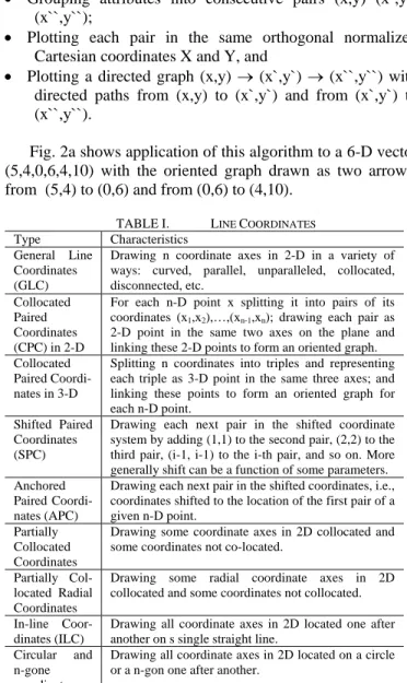
TABLE I. LINE COORDINATES

Type Characteristics General Line

Coordinates (GLC)

Drawing n coordinate axes in 2-D in a variety of ways: curved, parallel, unparalleled, collocated, disconnected, etc.

Collocated Paired Coordinates (CPC) in 2-D

For each n-D point x splitting it into pairs of its coordinates (x1,x2),…,(xn-1,xn); drawing each pair as

2-D point in the same two axes on the plane and linking these 2-D points to form an oriented graph. Collocated

Paired Coordi- nates in 3-D

Splitting n coordinates into triples and representing each triple as 3-D point in the same three axes; and linking these points to form an oriented graph for each n-D point.

Shifted Paired Coordinates (SPC)

Drawing each next pair in the shifted coordinate system by adding (1,1) to the second pair, (2,2) to the third pair, (i-1, i-1) to the i-th pair, and so on. More generally shift can be a function of some parameters. Anchored

Paired Coordi-nates (APC)

Drawing each next pair in the shifted coordinates, i.e., coordinates shifted to the location of the first pair of a given n-D point.

Partially Collocated Coordinates

Drawing some coordinate axes in 2D collocated and some coordinates not co-located.

Partially Col-located Radial Coordinates

Drawing some radial coordinate axes in 2D collocated and some coordinates not collocated. In-line

Coor-dinates (ILC)

Drawing all coordinate axes in 2D located one after another on s single straight line.

Circular and n-gone

coordinates

Drawing all coordinate axes in 2D located on a circle or a n-gon one after another.

The Shifted Paired Coordinates (SPC) show each next pair in the shifted coordinate system. The first pair (5,4) is drawn in the (X,Y) system. The next pair (0,6) is drawn not in the original system (X,Y), but in the shifted coordinate system denoted as (X+1,Y+1), where coordinate X is shifted up by 1, and coordinate Y is shifted to the right by 1. This means that the pair (0,6) in coordinates (X+1,Y+1) will be a pair (0,6)+(1.1)=(1,7) in the original coordinates (X,Y). For shift n and coordinates (X+n,Y+n) it is (a,b)(X+n,Y+n) = (a+n,b+n)(X,Y).

3

The pair (4,6) is drawn in the (X+2, Y+2) coordinates. For point (5,4,0,6,4,10), the graph includes the arrows: from (5,4) to (1,1)+(0,6)=(1,7) then from (1,7) to (2,2)+(4,10)=(6,12). See Fig. 2b.

The Anchored Paired Coordinates (APC) represent each next pair starting at the first pair that serves as an “anchor”. In the example above pairs (x`,y`) and (x``,y``) are represented as vectors that start at anchor point (x,y) with plotting vectors ((x,y), (x+x`,x+y`)) and ((x,y), (x+x``,x+y``)).

The graph of a 6-D point (1,1,1,1,1,1) in Partially Collocated Radial Coordinates is shown in Fig. 3 on the left as a blue triangle. The same 6-D point in the Cartesian Collocated Paired Coordinates on the right produced a much simpler graph as a single point. Fig. 3 illustrates the perceptual and cognitive differences between alternative 2-D representations of the same n-D data. Here a 2-D point is much simpler perceptually and cognitively than a tringle for the same 6-D point.

IV. GRAPHS IN GENERAL LINE COORDINATES

General Line Coordinates are constructed by drawing n

coordinate axes in 2-D in a variety of ways: curved, parallel, unparalleled, collocated, disconnected, etc. This definition

must be accompanied by an algorithm for constructing a 2-D graph that will represent an n-D point. Next, we present four algorithms

(a) 4-D point in collocated paired coordinates

(b) 4-D point in Shifted Paired Coordinates Point (6,12) is produced by adding (2,2) to (4,10).

(c) the same 4-D point as above in Parallel Coordinates

(d) In-line Coordinates

Fig.2. Data point (5,4,0,6,4,10) in different coordinate systems

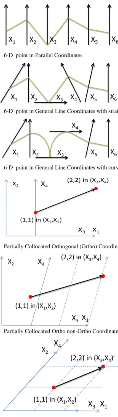
(a) 6-D point in Parallel Coordinates

(b) 6-D point in General Line Coordinates with straight lines

(c) 6-D point in General Line Coordinates with curves

(d) Partially Collocated Orthogonal (Ortho) Coordinates

(e) Partially CollocatedOrtho non-Ortho Coordinates

(d) Collocated non-Ortho Coordinates

Fig. 1 Examples of General Line Coordinates. (d),(e),(f) 4-D point (1,1,2,2) in different coordinate systems

X₁ X₂ X3 X4 X5 X6 X1 X2 X3 X4 X5 X6 X1 X2 X3 X4 X5 X6 X1 X2 X3 X4 (1,1) in (X1,X2) (2,2) in (X3,X4) X₁ X2 X₃ X₄ (1,1) in (X1,X2) (2,2) in (X3,X4)

X

X

X

X

X

X

X

X

X

x

_x

4

Fig. 3. 6-D point (1,1,1,1,1,1) in two X1-X6 coordinate systems (left – in

Radial Collocated Coordinates, right- in Cartesian Collocated Coordinates). Algorithm 1: Constructing a graph as a collection of oriented edges (arrows, vectors). Each edge is located on the respective coordinate Xi starting at the origin of this coordinate

and ending at point xi on Xi. See Fig. 4a. We will call this

algorithm a basic GLC graph constructing algorithm (GLC-B). Algorithm 2: Constructing a graph by connecting location of xi on Xi with the location of xi+1 on Xi+1, starting from i=1,

and ending at i=n. See Fig.4b. This is a generalization to GLC of the algorithm implemented in Parallel Coordinates (PC) [5]. Respectively we will call it as GLC-PC graph constructing algorithm.

(a) 6 coordinates and 6 vectors that represent a 6-D data point (0.75,0.5,0.7,0.6,0.7, 0.3)

(b) 6-D data point (0.75,0.5,0.7,0.6,0.7, 0.3) in GLC-PC

(c) 6-D data point (0.75,0.5,0.7,0.6,0.7, 0.3) in GLC-SC

(d) 6-D data point (0.75,0.5,0.7,0.6,0.7, 0.3) in GLC-CC

Fig.4.6-D data point (0.75,0.5,0.7,0.6,0.7,0.3) in different coordinate systems.

Algorithm 3: Constructing a graph by the algorithm as illustrated in Fig. 4c. It moves the start point of each vectors xi+1 to the end of vector xi. This algorithm is a generalization to

GLC of the algorithm implemented in the Star Coordinates (SC) [15]. Respectively we will call it as GLC-SC graph constructing algorithm.

Algorithm 4: Constructing a graph by the algorithm that is illustrated in Fig. 4d. It is a generalization to GLC of the algorithm implemented in the Collocated Coordinates (CC) [6] shown in Fig. 1d-f. Respectively, we will call is this algorithm the GLC-CC graph constructing algorithm.

Fig. 4 shows that algorithm 4 requires 3 points and 2 lines, but algorithm 1 requires 12 points and 6 lines for lossless representation of an n-D point. Algorithm 2 requires 6 points and 5 lines, and Algorithm 3 requires 7 points and 6 lines. In general, Algorithm 4 (GLC-CC) requires two times less points and lines than algorithms 1-3. This is a fundamental advantage

of GLC-CC algorithm from human cognitive viewpoint, because it simplifies pattern discovery by a naked eye. Below we present algorithms 1 and 4 more formally as a set of steps for graph generation.

Basic GLC graph construction algorithm (GLC-B) Step 1: Build GLC (see Fig. 5a for an example with n=6). Step 2: Select an n-D point, e.g., (7, 5, 6, 5, 6, 2).

Step 3: For each i (i=1:n) locate value xi in the coordinate

Xi (see Fig. 4a for an example), and define n vectors xi of

length xi from the origin of Xi that we denote as Oi.

GLC-CC graph construction algorithm

Step 1: Construct vectors {xi} by using basic GLC-B

algorithm.

Step 2: Compute the sum of vectors x1 and x2, x12=x1+x2

and then compute the point P1=O1+ x12. Next compute the sum

of vectors x3 and x4, x34=x1+x2 and the point P2=P1+x34. Repeat

this process by computing P3=P2+x56 and for all next i. For

even n the last point is Pn/2=Pn/2-1+xn-1,n (See Fig. 4d), for odd n

the last point is P(n+1)/2=P(n+1/2)-1+2xn.

Step 3: Build an oriented graph by connecting points {P}: P1=>P2=>…Pi-1=>Pi…=> … Pn. This graph can be closed by

adding edge Pn=> P1 .

Statement. The graph constructed by the GLC-CC algorithm has one-to-one mapping to n-D point X=(x1,x2,…xn)

and has less than a half of the nodes and edges than GLC-PC and GLC-SC.

Proof. The point P1 allows us to restore x1 by projecting it

to coordinate X1 as shown in Fig. 4d. Formally it can be

computed by representing the coordinate X1 as a vector X1, and

using a dot product of it with vector (P1-O1), (P1-O1)•X1.This

gives us a vector x1. Next, the property P1=O1+ x12= O1+ x1+x2

allows us to compute x2= P1-O1 - x1. In the same way by

projecting point P2 to X3, we get x3 and then using

P2=P1+x34=P1+x3 +x4 we restore x4= P2-P1- x3.Thesesteps are

continued for all points Pi until all xi are restored. The property

ofless than a half of the nodes and edges in GLC-CC, relative

X1 X6 X2 X3 X4 X₅ 1 1 1 1 1 X3 X2 X5 X4X6 X1 X1 X₂ X₃ X₄ X₅ X₆ x₁ x₂ x₃ x₄ x5 x6 X1 X₂ X₃ X₄ X₅ X₆ x₁ x₂ x₃ x₄ x₅ x6 X1 X₂ X₃ X₄ X₅ X₆ x₁ x2 x₃ x₄ x5 x6 X1 X₂ X₃ X₄ X₅ X₆ x₁ x2 x₃ x₄ x5 x₆ P₁ P₂ P₃

5

to GLC-PC and GLC-SC, follows directly from their definitions. Fig. 4 illustrates this property.

So far we had shown a cognitive advantage of the GLC-CC representation, which is its twice smaller footprint in 2-D, relative to GLC-PC and GLC-SC. This leads to much smaller occlusion when multiple n-D data are represented in 2-D. Below we show its other advantage – the ability to represent losslessly any n-D point X=(x1, x2,…, xn) as a single 2–D point

instead of a graph. The algorithm to produce this representation will be called the Single Point (SP) algorithm Steps of the Single Point algorithm.

Step 1: Select an arbitrary 2-D point A = (a1,a2) on the

plane. This point will be called the anchor 2-D point. Then selectthe n-D point (x1, x2,…, xn) that will be called the base

n-D point. Next select a set of positive constants c1,c2,…,cn

that will be used a lengths of coordinates X1,X2,…,Xn.

Step 2: Compute 2-D points O1 = (a1-x1,a2-x2) and

E1 = (a1-x1+c1, a2-x2). Coordinate line X1 is defined as vector

(O1, E1).

Step 3: Define points O2 = O1 and E2 = (a1-x1, a2-x2+c2).

Coordinate line X2 is defined as a vector (O2, E2).

Step 4: Repeat steps 2 and 3 for all other coordinates to build the coordinate system X1,X2,…,Xn.

This algorithm creates a Generalized Shifted Paired Coordinates (GSPC) system, where each next pair of coordinates is drawn in the shifted Cartesian coordinates. These coordinates are defined by parameters which are respective components of a base n-D point X and 2-D anchor point A. See Fig. 5.

Fig. 5. 6-D points (3,3,2,6,2,4) and (2,4,1,7,3,5) in X1-X6 coordinate system

build using point (2,4,1,7,3,5) as an anchor.

Statement. In the coordinate system X1,X2,…,Xn

constructed by the Single Point algorithm with the given base n-D point X=(x1, x2,,.., xn) and anchor 2-D point A, the n-D

point X is mapped one-to-one to a single 2-D point A by GLC-CC algorithm.

Proof. Consider coordinate X1 and a point located on X1

at the distance x1 from O1. According to Step 2 of SP

algorithm O1 = (a1-x1,a2-x2). Thus it is the point (a1-x1+x1,a2

-x2)= (a1,a2-x2). It is projection of pair (x1,x2) to X1 coordinate.

Similarly consider coordinate X2 and a point located on X2 at

the distance x2 from O1.

According to Step 2 of SP algorithm O2=(a1-x1,a2-x2). Thus

it is the point (a1-x1,a2-x2+x2)=(a1-x1,a2). It is projection of pair

(x1,x2) to X2 coordinate. Therefore, pair (x1,x2) is represented in

X1,X2 coordinate system as (a1,a2). In the same way the pair

(x3,x4) is also mapped to the point (a1,a2). The repeat of this

reasoning for all next pairs (xi,xi+1) will match them to the

same point (a1,a2) too. This concludes the proof. See Fig. 5 that

illustrates this proof for a 6-D point (2,4,1,7,3,5).

Another advantage of the combination of GLC-CC and SP algorithms is that all n-D points of an n-D hypercube around a given base n-D point X=(x1,x2,…,xn) are mapped to graphs

that located within a square defined by the square algorithm defined below.

In other words informally, n-D locality is converted to 2-D locality and wise versa, or, an n-D point Y is close to the base n-D point X if and only if the graph of Y is close to 2-D anchor point A.

Steps of Square algorithm

Step 1: Construct a hyper-cube H with center at the base point X=(x1,x2,…,xn) and distance d to its faces. Respectively

2n nodes N of this hypercube are (x1+αd,x2+αd,…,xn+αd),

where α = 1 or α = -1 depending on the node, e.g., (x1+d,x2+d,…,xn+d), (x1-d,x2-d,…,xn-d), (x1+d,x2-d,…,xn-d).

Step 2: Construct a square S around point (a1,a2) with

corners: (a1+d,a2+d), (a1+d,a2-d), (a1-d,a2+d), (a1-d,a2-d).

Statement (locality statement). All graphs N that represent nodes of hypercube H are within square S.

Proof. Consider the n-D node (x1+d,x2+d,…,xn+d) of H

where d is added to all coordinates of the n-D point X. This node is mapped to the 2-D point (a1+d,a2+d) which is a corner

of the square S. Similarly the node (x1-d,x2-d,…,xn-d) of H

where d is subtracted from all coordinates of X is mapped to the 2-D point (a1-d,a2-d) which is another corner of the square

S. In the same way the n-D node of the hypercube that contains pairs (x1+d,x2-d), (x3+d,x4-d),…, (xi+d,xi+1-d),…, (x n-1+d,xn-d) i.e., with positive d for odd coordinates (X1,X3,…)

and negative d for even coordinates (X2, X4, ….) is mapped to

the 2-D point (a1+d,a2-d). Similarly, a node with alternation of

positive and negative d in all such pairs (xi-d,xi+1+d) will be

mapped to (a1-d,a2+d). Both these points are also corners of

the square S.

If an n-D node of H includes two pairs such as (xi+d,xi+1+d)

and (xj+d,xj+1-d) then it is mapped to the graph that contains

two 2-D nodes (a1+d,a2+d) and (a1+d,a2-d) that are corners of

the square S. Similarly if an n-D node of H includes two other pairs (xk-d,xk+1+d) and (xm-d,xm+1-d) it is mapped to the

graph that contains two 2-D nodes (a1-d,a2+d) and (a1-d,a2-d)

that are two other corners of the square S. At most a hypercube n-D node has all these four types of pairs that can be present several times in it, and respectively all of them will be mapped to four corners of the 2-D square S.

These corners are 2-D nodes of the graph that represents this n-D node of the hypercube. Respectively, all edges of this graph will be within square S. Any other n-D point Y of the hypercube H has at least one coordinate that is less than this

(2,4,1,7,3,5) X1 X5 X3 X2 X4 X6 2 1 3 7 4 5 (3,3,2,6,2,4)

6

coordinate for some node Q of this hypercube. For example, let y1<q1 andyi=qi for all other i then all pairs (yi,yi+1), but the

first pair (y1,y2) will be mapped to the corners of the square S.

The first pair (y1,y2) will be mapped to the 2-D point, which is

inside of the square S because y1<q1. This concludes the proof.

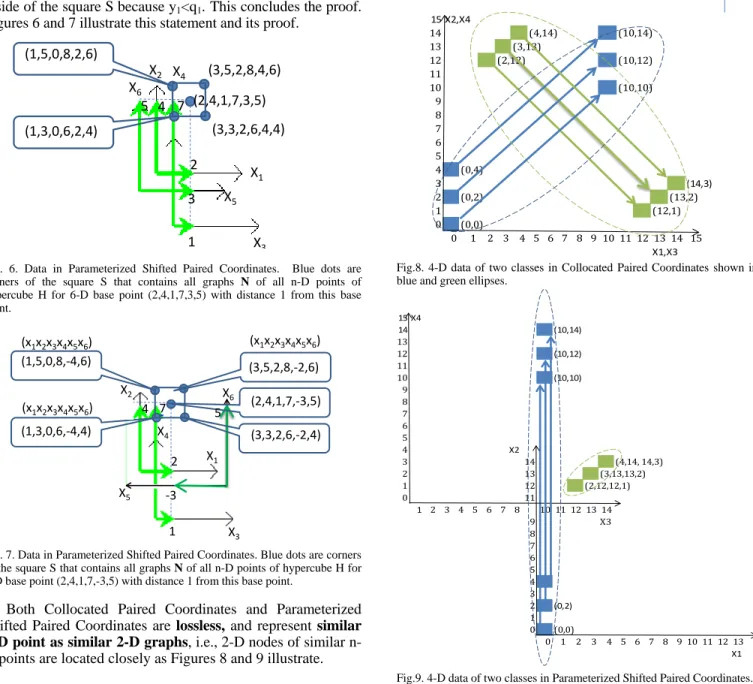
Figures 6 and 7 illustrate this statement and its proof.

Fig. 6. Data in Parameterized Shifted Paired Coordinates. Blue dots are corners of the square S that contains all graphs N of all n-D points of hypercube H for 6-D base point (2,4,1,7,3,5) with distance 1 from this base point.

Fig. 7. Data in Parameterized Shifted Paired Coordinates. Blue dots are corners of the square S that contains all graphs N of all n-D points of hypercube H for 6-D base point (2,4,1,7,-3,5) with distance 1 from this base point.

Both Collocated Paired Coordinates and Parameterized Shifted Paired Coordinates are lossless, and represent similar n-D point as similar 2-D graphs, i.e., 2-D nodes of similar n-D points are located closely as Figures 8 and 9 illustrate. Fig. 8 shows an example of 4-D data of two classes in Collocated Paired Coordinates in blue and green ellipses. Fig. 9 shows data from Fig. 8 in the Parameterized Shifted Paired Coordinates with 4-D point (3, 13,13,2) from the green class as the base point for parameterized shift.

Both Figs 8 and 9 show the separation of two classes, but in Fig. 9, the separation between these blue and green classes is much simpler than in Fig. 8. This is a demonstration of the promising advantages of parameterized shifted coordinates to simplify visual patterns of n-D data in 2-D in tasks such as clustering and supervised classification.

This gives the direction for future studies to solve a major challenge. This challenge is finding conditions where this

empirical observation can be converted into the provable property of simpler and less overlapped 2-D representation of non-intersecting hyper-ellipses, hyper-rectangles, and other shapes in n-D.

Fig.8. 4-D data of two classes in Collocated Paired Coordinates shown in blue and green ellipses.

Fig.9. 4-D data of two classes in Parameterized Shifted Paired Coordinates. V. REAL DATA VISUALIZATION

Fig. 10 shows the results of the comparison of all four coordinates for Iris data [4] that contain 150 4-D iris records. In contract with Parallel Coordinates (Fig. 10d), the new Collocated Paired visualizations (Fig.10abc) practically have no overlap for these data.

The iris-setosa class is clearly separated from the other two classes in these new visualizations. Note that these visualizations need only one 2-D segment to represent a 4-D data record. In contrast the Parallel Coordinates require three segments per 4-D record. The larger number of segments leads to more overlaps among lines in parallel coordinates. Other successful experiments with real world data are presented in [6,7]. (3,5,2,8,4,6) X1 X5 X3 X2 X4 X6 2 1 3 7 4 5 (2,4,1,7,3,5) (3,3,2,6,4,4) (1,5,0,8,2,6) (1,3,0,6,2,4) (3,5,2,8,-2,6) X1 X5 X3 X2 X4 X6 2 1 7 4 (2,4,1,7,-3,5) (3,3,2,6,-2,4) (1,5,0,8,-4,6) (1,3,0,6,-4,4) -3 (x1x2x3x4x5x6) (x1x2x3x4x5x6) (x1x2x3x4x5x6) 5 15 X2,X4 14 (4,14) (10,14) 13 (3,13) 12 (2,12) (10,12) 11 10 (10,10) 9 8 7 6 5 4 (0,4) 3 (14,3) 2 (0,2) (13,2) 1 (12,1) 0 (0,0) 0 1 2 3 4 5 6 7 8 9 10 11 12 13 14 15 X1,X3 15 X4 14 (10,14) 13 12 (10,12) 11 10 (10,10) 9 8 7 6 5 4 X2 3 14 (4,14, 14,3) 2 13 (3,13,13,2) 1 12 (2,12,12,1) 0 11 1 2 3 4 5 6 7 8 10 11 12 13 14 9 X3 8 7 6 5 4 3 2 (0,2) 1 0 (0,0) 0 1 2 3 4 5 6 7 8 9 10 11 12 13 X1

7

(a) Collocated Paired Coordinates (b) Anchored Paired Coordinates.

(c) Shifted Paired Coordinates (d) Parallel Coordinates Figure 10. Iris data (red Iris-setosa class)

VI.SUPER-INTELLIGENCE FOR HIGH-DIMENSIONAL DATA The results presented above create an exciting opportunity for progress in super-intelligence studies. While significant progress in AI, CI and Machine Leaning improved human abilities to discover patterns in n-D data the direct human cognitive abilities to do this with a naked eye are extremely limited to relatively small 2-D and 3-D datasets.

Lifting this human cognitive limitation is in a drastic contrast with the opposite goal of reaching human-level machine intelligence for human abilities, which is the goal of other aspects of AI, CI, and Cognitive Science. This opposite goal is deciphering the brain’s existing cognitive abilities and mimicking human intelligence that use a naked eye very successfully to recognize and discover visual patterns, e.g., faces and facial expressions, in our physical 3-D world.

Thus we need both the deciphering of the brain and the enhancing of it to be able to deal with abstract high-dimensional data as it does with 2-D and 3-D data. Compare it to building a machine that will fly as a bird. It is difficult to decipher the mechanism of bird flying. The history of aviation had shown that direct attempts to mimic it failed many times.

Next, the machine that intends only to mimic a flying bird will be limited. It will not fly to the Moon and Planets. For flying that far a machine with super-bird flying capabilities is needed. Similarly deciphering brain’s ability to work visually with 2-D data hardly will give us a way to build a super-intelligence to deal with large abstract n-D data. This is a separate and very challenging task. Evolution has developed our brain in a particular form to adapt to a particular physical 3-D environment that did not include abstract high-dimensional data (n-D data) to be analyzed until the very recent Big data era.

This separate task requires ideas beyond what is on the surface when humans solve their typical cognitive tasks in 2-D

and 3-D. In the same way exploring how a bird is flying hardly will help to build a rocket to fly to the Moon. For the flight to the Moon we need to discover more general flying principles. Similarly for dealing with Big n-D data we need to discover more general cognitive principles than we use for 2-D and 3-D data.

Is it always more difficult to discover more general principles than more specific ones? The history of the science tells us that it is not always the case. The modern flight theory that includes the propulsion theory and aerodynamics explains not only bird flight, but also rocket and aircraft flights. However this more general theory does not tell us anything about the physiology of bird flight at the level of muscles and the bird brain control of the flight. Thus higher generality does not mean abilities to explain all aspects of the bird flight. However it can help to discover and understand a mechanism of other related activities. For instance, the propulsion theory allows the understanding of an octopus motion. In our case it is discovering cognitive principles to deal with n-D data.

This brings us to the important point that for understanding some fundamental brain cognitive principles it is not necessary to study the brain itself first. Respectively to build such more general theory we can work on the task that brain does not support well, which is dealing with n-D abstract data. The goal is to understand and enhance brain’s capability to deal with such n-D data. It includes experiments with the same n-D data where a human recognizes or not recognizes the pattern depending on 2-D lossless representation of these n-D data. These experiments can tell about human abstract pattern recognition abilities providing data to build a cognitive model in a form of a discrimination function that separates 2-D lossless representations of n-D data.

After a discrimination function is built, the next question is: “What is the mental process in the brain behind this ability or inability?” The common approach in such tasks is collecting and analyzing the functional MRI data when the task is solved by subjects. In [18] functional MRI was used to measure activity in a higher object processing area, the lateral occipital complex, and in primary visual cortex in response to visual elements that were either grouped into objects or randomly arranged. These authors observed significant activity increases in the lateral occipital complex and concurrent reductions of activity in primary visual cortex when elements formed coherent shapes. Based on this observation they suggested that activity in early visual areas is reduced as a result of grouping processes performed in higher areas. These findings were used as an evidence for the brain predictive coding models of vision [17,20] that postulate that inferences of high-level areas are subtracted from incoming sensory information in lower areas through cortical feedback. Note that this study was conducted for 2-D and 3-D shapes such as shown in Fig. 11 without any relation to n-D data.

The predictive coding models of vision represent one side of two fundamental alternatives: local and distributed representation models/hypotheses for the brain to be

8

biologically-adequate representations for observed high-level structures and cognitively-adequate models. There are several distributed representation cognitive models with bottom-up and top-down signals [14, 17] including the dynamic logic model that we advocate [8] because if its ability to overcome combinatorial complexity. On the other hand while current deep leaning large Neural Networks may not be biologically-adequate their applied results are impressive.

Fig. 11. Examples of different stimulus conditions [18]

VII. CONCLUSION AND FUTURE STUDIES

This paper described the proposed new algorithms for lossless visual representation of high-dimensional data and their connections with human super-intelligence challenges. We interpret these algorithms as cognitive algorithms that enhance human cognitive abilities to deal with modern Big data high-dimensional challenges. The paper focused on Generalized Shifted Paired Coordinates as a subset of General Line Coordinates. The advantages of these coordinates have been shown both mathematically and on the data. These advantages guide future studies to solve a major challenge. This challenge is finding conditions for a provable property of simpler and less overlapped lossless 2-D representation of the non-intersecting hyper-ellipses, hyper-rectangles, and other shapes in n-D.

The advantage of a wide class of General Line Coordinates is that it allows multiple different visualizations of the same data with the different perceptual and cognitive characteristics. This multiplicity increases the chances that humans will be able to reveal the hidden n-D patterns in these visualizations. It is not realistic to expect that a single visualization will do this for all possible data and all humans. A full classification of general line coordinates for cognitively efficient n-D data visualization is a task for future research as well as deeper links with Machine Learning to be able to build visually the learning algorithms using visual means in GLC such as Decision Trees. This is an area of future studies for the design of more complete processes and for expanding to other data mining/machine learning methods.

Other future studies include gaze analysis: when humans analyze visual representations of abstract n-D data and discover n-D patterns. While eyes provide initial input of such visual information, visual perception, and cognition deeply involve the brain. Therefore the gaze analysis will help to look deeper into this complex process. Combining eye tracking methodology, mathematical models from different fields, and the behavioral information which emerges in the analysis of n-D data will be a source of new knowledge of the cognitive processes. This will include future experiments that compare

observers' performance in discovering n-D data patterns by analyzing 2-D graphs as a function of their fixations and simulations by computations of these fixations.

These future studies will also help to reveal the individual variability among the people in their perceptual and cognitive abilities for recognizing the abstract forms. These future studies will provide a new way to understand visual and cognitive perception, as well as improve the accuracy, increase efficiency, and decrease the cost of n-D data analysis.

REFERENCES

[1] Bertini E., Tatu, A., Keim, D., Quality metrics in high-dimensional data visualization: An overview and systematization, IEEE Tr. on Visualization and Computer Graphics, 17 (12), pp. 2203 – 2212, 2011 [2] Grishin V., Kovalerchuk, B., Multidimensional collaborative lossless

visualization: experimental study, CDVE 2014, Seattle, Sept 2014. Luo (Ed.): CDVE 2014, LNCS 8683, pp. 27–35, Springer, 2014.

[3] Hoffman P., Grinstein G.,, Survey of Visualizations for High-Dimensional Data Mining, In: Information Visualization in Data Mining and Knowledge Discovery, Eds. U. Fayyad, A. Wierse, G. Grinstein, pp. 44-82, Academic Press, 2002.

[4] Iris Data Set, Machine Learning Repository, 1988. https://archive.ics.uci.edu/ml/datasets/Iris

[5] Inselberg, A., Parallel Coordinates: Visual Multidimensional Geometry and its Applications. Springer, 2009.

[6] B. Kovalerchuk, Visualization of multidimensional data with collocated paired coordinates and general line coordinates, Proc. SPIE 9017, Visualization and Data Analysis 2014, 90170I.

[7] Kovalerchuk B., Grishin V, Collaborative lossless visualization of n-D data by collocated paired coordinates, CDVE 2014, Seattle, Sept 2014, Y. Luo (Ed.): CDVE 2014, LNCS 8683, pp. 19–26, Springer Switzerland, 2014.

[8] Kovalerchuk B., Perlovsky L., Wheeler G., Modeling of Phenomena and Dynamic Logic of Phenomena, Journal of Applied Non-classical Logics, 22(1): 51-82, 2012.

[9] Simov S., Bohlen M., Mazeika A. (Eds), Visual Data Mining, Springer, 2008

[10] Tergan S., Keller T., (eds) Knowledge and Information Visualization, Springer, 2005

[11] M. Ward, G. Grinstein, and D. Keim, Interactive Data Visualization: foundations, techniques, and applications, A K Peters, Ltd. Natick, MA, 2010.

[12] Wong, P., Bergeron, R., 30 Years of Multidimensional Multivariate Visualization. In G. M. Nielson, H. Hagan, and H. Muller (Eds), Scientific Visualization - Overviews, Methodologies and Techniques, pages 3-33, IEEE Computer Society Press, 1997.

[13] Hibbard, B. Super-Intelligent Machines. Kluwer, 2002

[14] Carpenter, G. A., and Grossberg, S. (2015). Adaptive resonance theory. Encyclopedia of Machine Learning and Data Mining. C. Sammut and G. Webb, Eds. Berlin: Springer-Verlag, 2014.

[15] Kandogan, E., Visualizing multi-dimensional clusters, trends, and outliers using star coordinates, Proc. 7th ACM SIGKDD International conference on Knowledge discovery and data mining, pp. 107-116, 2001.

[16] Michelucci, P., Dickinson, J. L. The power of crowds. Science, 2015; 351 (6268): 32 DOI: 10.1126/science.aad6499

[17] Mumford, D., On the computational architecture of the neocortex. II. The role of cortico-cortical loops.Biol. Cybern. 66, 241–251, 1992. [18] Murray S., Kersten D., Olshausen B., Schrater P., Woods D., Shape

perception reduces activity in human primary visual cortex, 15164– 15169, PNAS, Nov.12, 2002, vol. 99, no. 23,

www.pnas.orgycgiydoiy10.1073ypnas.192579399 [19] Superintelligence, Wikipedia, 11/12/2015

https://en.wikipedia.org/wiki/Superintelligence

[20] Rao, R. P., Ballard, D. H. , Predictive coding in the visual cortex: a functional interpretation of some extra-classical receptive-field effects, Nat. Neuroscience. 2, 79–87, 1999