J
ENA
E
CONOMIC
R
ESEARCH
P
APERS
# 2009 – 091
Accuracy, Unbiasedness and Efficiency of Professional
Macroeconomic Forecasts:
An empirical Comparison for the G7
by
Jonas Dovern
Johannes Weisser
www.jenecon.de ISSN 1864-7057
The JENA ECONOMIC RESEARCH PAPERS is a joint publication of the Friedrich
Schiller University and the Max Planck Institute of Economics, Jena, Germany. For editorial correspondence please contact [email protected]. Impressum:
Friedrich Schiller University Jena Max Planck Institute of Economics
Carl-Zeiss-Str. 3 Kahlaische Str. 10
D-07743 Jena D-07745 Jena
ACCURACY, UNBIASEDNESS AND EFFICIENCY OF PROFESSIONAL MACROECONOMIC FORECASTS:
AN EMPIRICAL COMPARISON FOR THE G7
JONAS DOVERN AND JOHANNES WEISSER November 16, 2009
Abstract. In this paper, we use survey data to analyze the accuracy, unbiasedness,
and the efficiency of professional macroeconomic forecasts. We analyze a large panel of individual forecasts that has not been analyzed in the literature so far. We provide evidence on the properties of forecasts for all G7 counties and for four different macro-economic variables. Our results show a high degree of dispersion of forecast accuracy across forecasters. We also find that there are large differences in the performance of forecasters not only across countries but also across different macroeconomic variables. In general, forecasts tend to be biased in situations where forecasters have to respond to large structural shocks or gradual changes in the trend of a variable. Furthermore, while a sizable fraction of forecasters seem to smooth their GDP forecasts significantly, this does not apply to forecasts made for other macroeconomic variables.
Keywords: Evaluating forecasts, Macroeconomic Forecasting, Rationality, Survey Data, Fixed-Event Forecasts
JEL Classification: C25,E32,E37
1. Introduction
In this paper, we use survey data to analyze the accuracy, efficiency, and unbiasedness of professional macroeconomic forecasts in the G7 countries. We analyze individual forecasts from large cross sections of professional forecasters, enabling us to throw light on the heterogeneity across forecasters.1
Moreover, our results are not affected by problems that arise from the use of average, so-called consensus, forecasts (e.g., aggregation bias). Our large data set has not been exhaustively used in the literature before. By using this large amount of disaggregate data on individual macroeconomic forecasts, we are able to
Jonas Dovern, Kiel Economics Research & Forecasting GmbH & Co. KG, Fraunhoferstr. 13, 24118 Kiel, Germany, Tel: 0049-431-530349-7; [email protected]. Johannes Weisser, Max Planck Institute of Economics, [email protected]. The views presented in this paper reflect the authors’ opinion, and do not necessarily coincide with those of the Max Planck Institute of Economics. We are grateful to Helmut Herwartz, Christian Merkl, and two anonymous referees as well as to all participants of the Brown-Bag Seminar at Kiel University for valuable comments and suggestions. Adelheid Baker provided valuable support.
1For a comparison of results for individual and average forecasts, see a previous version of this paper
provide a much broader evidence base on the properties of macroeconomic forecasts than has so far been available in the literature.
A weak point of the empirical literature, which uses survey data to assess the efficiency or unbiasedness of macroeconomic forecasts, is that there is only a limited number of non-U.S. data sets providing information on forecasts. Consequently, existing evidence is predominantly based on U.S. data. Notable exceptions are Harvey et al. (2001), who ana-lyze a set of selected individual forecasts for the U.K. from the survey data set provided by
Consensus Economics; Gallo et al. (2002), who analyze the evolution of macroeconomic forecasts for the U.S., the U.K., and Japan; Bowles et al. (2007), who analyze the perfor-mance of forecasts summarized in the Survey of Professional Forecasters conducted by the European Central Bank; Isiklar et al. (2006) or Ager et al. (2009), who use data from the
Consensus Economics data set on forecasts for a set of industrialized countries; Loungani (2001), who additionally examines data for developing countries; Timmermann (2007), who analyzes the performance of IMF forecasts from the World Economic Outlook for various countries; Batchelor (2001), who compares the forecasts made by the IMF and the OECD to private sector forecasts; and Boero et al. (2008a,b), who analyze forecasts from the Bank of England Survey of External Forecasters. However, all existing international studies, with the exception of Harvey et al. (2001) and Boero et al. (2008a,b), make ex-clusive use of consensus forecasts rather than analyzing individual forecasts – these three studies are, however, confined to U.K. data sets. The purpose of our paper is to fill this gap, covering individual forecasts for all G7 countries and four macroeconomic variables. Our results are based on an approach commonly used in the literature to model the structure of macroeconomic forecasts, dating back to early contributions by Ball (1962), Mincer and Zarnowitz (1969), Figlewski and Wachtel (1981), or Nordhaus (1987), who introduced the basic modeling framework for analyzing fixed event forecasts.2 A sequence
of fixed event forecasts consists of consecutively formed forecasts for the same event (such as an annual figure for a macroeconomic variable). The data we use below is of this type.
2Pesaran and Weale (2006) and Stekler (2002) present concise summaries of the commonly used
ap-proaches. The latter contribution also provides an overview of the most prominent survey data sets used in empirical research on forecast efficiency.
Some more recent contributions have proposed to improve the econometric approach for testing the rationality of such large panels of fixed event forecasts. These include Keane and Runkle (1990) and Batchelor and Dua (1990), who introduce an analysis in a panel framework using the Generalized Methods of Moments (GMM) method, or Davies and Lahiri (1995), who develop a framework for analyzing three-dimensional panels of survey data, enabling the use of information along all dimensions. To ensure that our results are comparable to existing studies, we closely follow the approach suggested by Davies and Lahiri (1995), and recently used by Clements et al. (2007), Boero et al. (2008a), and Ager et al. (2009), and suggest only minor modifications to the econometric framework.
of the survey and test whether they are unbiased and efficient. Assuming that forecast accuracy is the only objective of a forecaster and that her loss function is symmetric and increases with the forecast error, the latter two properties are inevitable features of a rational forecast. Regarding this point, it should be noted, however, that there are also arguments against the assumption that published forecasts reflect true expectations and are meant to minimize a loss function of the described form. Some of these arguments are as follows. First, forecasters might seek to maximize public attention. In this case, an unbiased forecast is not optimal anymore, since the utility of the forecaster depends on more than one argument (Laster et al., 1999). Second, forecasters might produce a so-called “intentional” forecast in some situations (Stege, 1989). A forecaster could, for example, predict a specific event to provoke a policy action that actually prevents the occurrence of the event. Third, forecasters might have asymmetric loss functions (Capis-tran and Timmermann, 2006, Boero et al., 2008a). These could have different weights concerning a possible over- or underestimation of an outcome. We believe, however, that these arguments are not a priori strong, particularly because in the data set we use the identity of the panelists are revealed. We therefore abstract from these issues and start this paper from the null hypothesis that it is in the forecasters’ best interest to provide unbiased and efficient forecasts.
Our findings show that the dispersion of forecast accuracy across panelists is surprisingly high for most (of the) countries and variables examined in this paper. We also find that
there are large differences in the performance (in terms of accuracy, unbiasedness, and efficiency) of forecasters not only across countries but also across different macroeconomic variables. In general, the forecasts for inflation are mostly consistent with the hypothesis of unbiased and efficient forecasts. Furthermore, forecasts tend to be biased in situations where forecasters have to recognize large structural shocks or gradual changes in the trend component of a variable.
The remainder of this paper is structured as follows. Section??presents a brief overview of the data set we use and a first visual inspection of the data. Section ?? illustrates the econometric framework used by us to model the forecast errors, and how tests on the unbiasedness and efficiency of forecasts can be derived. Section 3 discusses the hetero-geneity of accuracy of individual forecasts. Section 4 presents the empirical results on the unbiasedness of individual forecasts. Section 5 presents the empirical results on the efficiency of individual forecasts. Section 6 concludes.
In this paper, we rely on data from the surveys conducted by Consensus Economics, a London-based firm.3
Each month, starting in October 1989, Consensus Economics polls institutions like investment banks or economic research institutes about their forecasts for the most common macroeconomic variables. The largest samples of panelists are available for the G7 countries, on which we concentrate in this paper.4
A considerable advantage of the data set is that the data are comparable across countries as well as panelists.
Due to the fact that Consensus Economics asks the panelists to report their forecasts for the annual figures of the variables, the panel data set has a rather complex structure in that observations are correlated across several dimensions, as shown below. More specifically, the panel has a three-dimensional structure of the kind introduced in Davies and Lahiri (1995). For each country and variable we have an N T H-dimensional vector
3Information from the Consensus Economics data set have been used in a sequence of papers in recent
years to analyze the properties of macroeconomic forecasts. Most contributions, however, consider only data on average forecasts but do not analyze individual forecasts. Notable exceptions are Lahiri and Sheng (2008), who propose a model for disagreement among forecasters and estimate this based on individual forecasts on GDP growth from the Consensus Economics data set; Batchelor (2007), who uses a similar disaggregated data set to analyze the bias in forecasts for GDP growth; Dovern et al. (2009), who analyze the dispersion of macroeconomic forecasts; and, to some extent, Harvey et al. (2001), who analyze the properties of forecasts made by a selected group of panelists from theConsensus Economics data for the U.K.
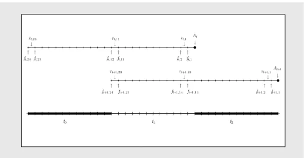
Figure 1. Forecast Data Structure
Notes: This shows schematically the sequence of forecast (ft,h) and forecast revisions (rt,h)
of one forecaster for the realizations of a variable in two consecutive years (t1 andt2).
of forecasts for T years made by N forecasters with forecast horizons ranging from 1 to
H months. In other words, for each year a sequence of H forecasts is collected from each forecaster, starting H months before the year ends and ending with the last month of that respective year. In our case, we have a sequence of H = 24 forecasts from each panelist for each variable’s annual figures. In our sample, we include forecasts for the years 1991 – 2005, i.e., T = 15 in our analysis. The number of panelists covered by the data set varies considerably across countries but also over time; however, usually N ≥ 10 even for the smaller countries. Figure 1 shows a schematic diagram of the forecast structure for one panelist and two consecutive target years.
We concentrate on forecasts for four variables: the annual growth rate of gross do-mestic product (GDP), the annual inflation rate, and the annual growth rates of private consumption expenditure and industrial production, respectively. It is important to note that some changes occurred in the definition of the target variables in some of the coun-tries. More specifically, while the inflation forecasts refer to the consumer price inflation in general, the relevant figure which had to be forecasted in the U.K. referred to the
Retail Price Index during the first period of our sample. Forecasts for CPI inflation in the U.K. were introduced in 2004.5 Furthermore, forecasters were asked to target the annual growth rate of the gross national product (GNP) rather than that of the gross domestic product (GDP) in Germany and Japan until 1992 and 1993, respectively. With regard to the German forecast, there is another break in the data due to the switch from data for former West Germany to data for reunified Germany. In our data set, forecasts for GDP growth and inflation refer to West Germany until 1996; for forecasts on private consumption expenditures and industrial production, the change was made in 1995.
A feature of the data we are concerned with is given by the fact that the record of most of the forecasters includes a set of missing values, i.e., the panel is heavily unbalanced. There are two reasons for this. First, the set of panelists engaged in the Consensus Economics survey changes continuously. Hence there are some forecasters entering the panel at a later stage, while others leave the panel after the first part of the period covered by our data set. Second, some forecasters do not submit their forecasts on a regular basis, i.e., they do not submit them for certain months. To minimize the reduction of our data base due to this aspect, we interpolate a missing value when a forecast is unavailable for one month and the two adjacent forecasts are equal to each other. Formally, if fi,t,h is
missingand fi,t,h+1 =fi,t,h−1, we set the missing forecast equal tofi,t,h+1. For the analysis
below, we include those panelists in the sample who made a forecast at more than 50% of the possible dates. We thereby avoid the influence of small sample problems which could arise from those panelists who submitted only a few forecasts.6
A final issue regarding data concerns the realizations we use to evaluate the forecast errors. For the evaluation of macroeconomic forecasts, it has become standard in the literature to use data from the initial releases rather than revised ex post data (see, e.g., Croushore, 2006). Following this approach, we compute forecast errors based on the historical data as listed in the publications of Consensus Economics in May of each subsequent year, respectively, since these data vintages should reflect the initial releases
5An additional change occurred in May 1997 when the underlying Retail Price Index changed to a version
that excludes interest payments on mortgages.
6The threshold of 50% is, of course, arbitrary. Results for the included panelists are, however, robust to
for all cases. To give an example: we use the realizations of variables for 1996, as reported together with the survey results by Consensus Economics in May 1997, to evaluate all forecasts that have been made for a variable’s realization in 1996 for the years 1995 and 1996.
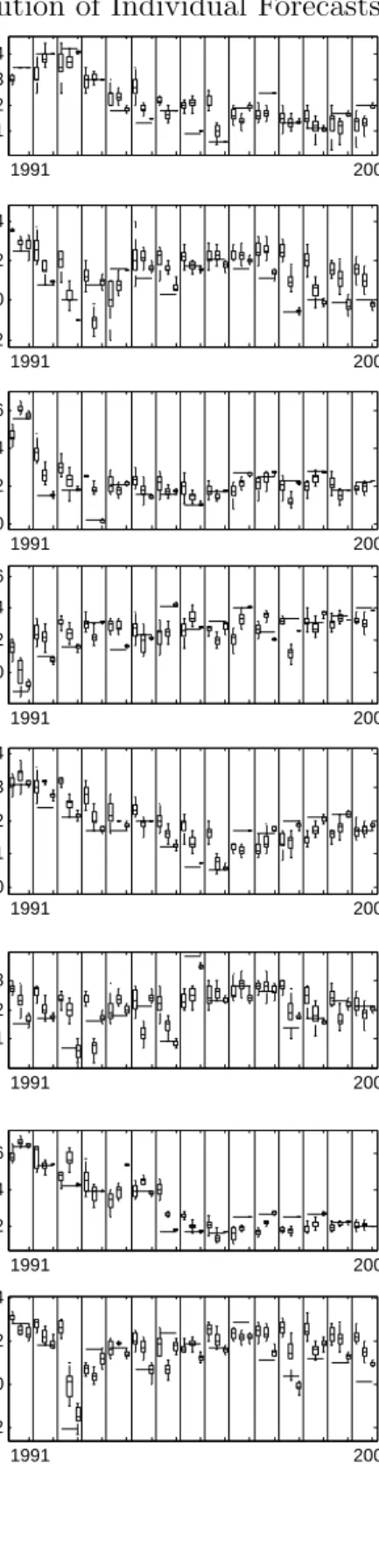
Figure 2 shows these first data releases together with three Box-Whisker plots for each year that depict the distribution of forecasts for h = 24,12,1, respectively. Four aspects are clear from a visual inspection of the data. First, the forecast dispersion diminishes considerably when the forecast horizon approaches zero, i.e., the height of the box is usually largest for h = 24 and smallest for h = 1. Second, quite often even the last forecasts made for a specific year (with h = 1) are quite distant from the first data releases. Third, the majority of forecasters seem to lag behind when structural changes occur, i.e., when the unconditional expectation of a variable changes. This is exemplarily shown in the graph for inflation forecasts in the U.K. for the period between 1991 and 1994; the forecasts for real GDP growth and the growth rate of private consumption in the U.S. between 1996 and 2000; or the forecasts for real GDP growth in Germany between 2001 and 2003. Finally, the figure illustrates the well-known phenomenon that turning points are usually not forecasted in advance. This is particularly pronounced for turning points in real economic activity, as can be seen, for instance, in the case of the recessions in Germany (1993), Canada (1991), Italy (1993), the U.K. (1991), or the U.S. (2001).
2. Model Framework
2.1. A Structural Model for Forecast Errors. As mentioned above, our panel pos-sesses a three dimensional structure of the kind introduced in Davies and Lahiri (1995). Following conventional notation, we denote a forecast made by forecaster i = 1, . . . , N
with a forecast horizon of h = 1, . . . , H for the realization of the variable of interest in target year t = 1, . . . , T by fi,t,h. The stacked vector of forecasts is denoted by
F = [f1,1,H, f1,1,H−1, . . . , f1,1,1, f1,2,H, . . . , f1,T ,1, f2,1,H, . . . , fN,T,1]
0
and NTH entries long. Following Davies and Lahiri (1995), we assume that the forecast error for each forecast
Figure 2. Data Realizations and Distribution of Individual Forecasts 1991 2005 −2 0 2 4 Germany−GDP 1991 2005 −2 0 2 4 Canada−GDP 1991 2005 0 2 4 France−GDP 1991 2005 0 1 2 3 Italy−GDP 1991 2005 1 2 3 4 Germany−INFL 1991 2005 0 2 4 6 Canada−INFL 1991 2005 0 1 2 3 4 France−INFL 1991 2005 2 4 6 Italy−INFL 1991 2005 −5 0 5 Germany−IP 1991 2005 −5 0 5 Canada−IP 1991 2005 −5 0 5 France−IP 1991 2005 −4 −2 0 2 4 6 Italy−IP 1991 2005 −2 0 2 4 Germany−CONS 1991 2005 0 2 4 6 Canada−CONS 1991 2005 1 2 3 France−CONS 1991 2005 −2 0 2 4 Italy−CONS
can be decomposed into three different parts
ei,t,h ≡At−fi,t,h =φi+λt,h+i,t,h ,
Figure 2. Data Realizations and Distribution of Individual Forecasts (Continued) 1991 2005 −2 0 2 4 Japan−GDP 1991 2005 −2 0 2 4 U.K.−GDP 1991 2005 0 2 4 6 U.S.−GDP 1991 2005 −1 0 1 2 3 Japan−INFL 1991 2005 2 4 6 U.K.−INFL 1991 2005 1 2 3 4 5 U.S.−INFL 1991 2005 −5 0 5 Japan−IP 1991 2005 −5 0 5 U.K.−IP 1991 2005 −5 0 5 U.S.−IP 1991 2005 −2 0 2 4 Japan−CONS 1991 2005 −2 0 2 4 U.K.−CONS 1991 2005 0 2 4 U.S.−CONS
Notes: First data releases are represented by solid lines. The items of the Box-Whisker-plots have the usual meaning. The box indicates the upper and lower quartile, whereas the Whiskers indicate the remaining distribution of observations but are restricted to be 1.5 times as long as the interquartile range. Outlier are not displayed to retain clarity.
where At denotes the realization of a variable for year t. The first error component φi is
the individual bias of the forecasts made by forecasteri. The second error componentλt,h
is common to all forecasters and reflects the occurrence of macroeconomic shocks that hit an economy between the date at which the forecasts are made and the end of year t. Following the literature, we assume that these shocks are cumulated over the hmonths in an arithmetic way, so that this component can be written asλt,h =
Ph
k=1ut,k. We assume
that ut,h is distributed with a zero mean and a variance of σ2u. Since ut,h and ut+1,h+12
The third error componenti,t,h refers to the forecaster specific part of the forecast error
(apart of the constant bias). The literature proposes two alternative ways to model this error. On the one hand, it can be seen as an independently and identically distributed (iid) shock. This is the view taken for the estimation in Davies and Lahiri (1995). On the other hand, Davies and Lahiri mention that one could assume that over time each forecaster receives a flow of private information on the outcome, which successively decreases her individual forecasting error. Under this assumption, one can model the forecaster-specific error component as i,t,h =
Ph
k=1ηi,t,k, where the ηi,t,k are distributed with mean 0 and
varianceσi2. Again,ηi,t,kandηi,t+1,k+12have a non-zero correlation, since these information
shocks occur at the same point in time.
It is clear that the two model variants for i,t,h have very different implications. In
the first case, the forecaster-specific error components are assumed to be a white noise process, while, in the second case, they are assumed to follow a random walk for each target year t. In the first case, there would be no correlation between consecutive forecaster-specific error components, while, in the second case, the autocorrelation would be high and decay only slowly for higher distances between two forecast errors for the same target year. Intuitively, the second model is much more attractive: consider a forecaster whose forecast is above the consensus forecast in one month. Is it not very likely that he will publish an above-average forecast also in the following month? That is, it would be very strange to think that individual forecasts fluctuate randomly around the consensus forecast without any persistence. Rather, a forecaster is likely to be persistently more optimistic or pessimistic than the average for some time. This behavior would be better captured by the second model, implying a high autocorrelation of the individual errors.
Ultimately, choosing from the two alternatives is a matter of empirical facts. In our data set, the estimates of the forecaster-specific error components, say ˆi,t,h, show a fairly high
degree of autocorrelation. The empirical autocorrelation functions are usually declining slowly and approach zero only after about twelve months. So we usually prefer the second model to the first based on Bayesian information criteria. In this respect, our econometric framework deviates from other studies.
2.2. A Test of Unbiasedness. Testing the unbiasedness of forecaster i is equivalent to testing whether φi = 0 in (1). We can examine this hypothesis by testing the zero
restriction on the elements of Φ = [φ1, . . . , φN]
0 in e=A−F = Φ⊗iT H+λ+ | {z } =ν , (2)
where e is the vector of stacked forecast errors, A is given by iN ⊗(A+⊗iH) with A+ =
(A1, A2, . . . , AT)
0
and iT H, iN and iH are vector of ones of dimension T H, N and H
respectively.7 λ and are vectors of length N T H in which we stack the appropriate λt,h
and i,t,h respectively.
Now, while a simple OLS regression gives consistent point estimates for the bias, we cannot base our inference on the OLS standard errors, since the elements of ν are clearly not iid due to the special correlation structure caused by the structure of the panel data set. Davies and Lahiri (1995) show that it is neither diagonal nor homoscedastic. Recalling that due to our assumption about the individual errors our specification differs from their model, we formally have the following elements of Σ = E[νν0] for two forecasters, say i
and j:
Cov(νi,t1,h1, νj,t2,h2) =Cov
h1 X k=1 ut1,k+ h1 X k=1 ηi,t1,k, h2 X k=1 ut2,k+ h2 X k=1 ηj,t2,k ! (3) Cov(νi,t1,h1, νj,t2,h2) = min{h1, h2}[σu2+σi2] ifi=j, t1 =t2, h1 =h2 min{h1, h2 −12}[σu2+σi2] ifi=j, t1 =t2−1, h2 ≥12 min{h1, h2}σ2u ifi6=j, t1 =t2, h1 =h2 min{h1, h2 −12}σu2 ifi6=j, t1 =t2−1, h2 ≥12 0 else
Clearly, the different non-zero cases deserve some more explanation. The forecast errors
ν are correlated across several dimensions. First, they are correlated within the maximum
forecast horizon H sinceλt,h and i,t,h are the accumulation of period-specific shocks; this
refers to the first case shown in (3). Second, the forecast errors are correlated between subsequent years since the forecast horizons are of overlapping nature; this refers to the second case shown in (3). Finally, the forecast errors are correlated across different forecasters, since forecast errors are produced at the same time and are all subject to the same subsequent aggregate shocks summarized by λt,h; this refers to the third and fourth
case shown in (3).
Given Σ, the covariance matrix of the Generalized Methods of Moments (GMM) esti-mator is given by V ar( ˆΦ) = [(IN ⊗iT H)0(IN ⊗iT H)] −1 [(IN⊗iT H)0Σ(IN⊗iT H)] [(IN ⊗iT H)0(IN⊗iT H)] −1 (4)
and can be used to derive valid t-statistics for testing φi = 0. Naturally, Σ is not observed
and has to be replaced by a consistent estimate, say ˆΣ, before computation of the test statistics is possible.
Though Σ has a complicated pattern, it depends only on N + 1 parameters, namely
σ2
1, . . . , σN2 and σu2. Davies and Lahiri (1995) propose to obtain a consistent estimate by
first estimating these N + 1 parameters and then replacing the parameters in Σ by the corresponding estimates. We will follow this approach. Note that an estimator of φi is
simply given by the average forecast error of forecaster i and that we can estimate the two other parts of the forecasts errors by
ˆ λt,h = 1 N N X i=1 At−fi,t,h−φˆi (5) and ˆ i,t,h =At−fi,t,h−φˆi−λˆt,h . (6)
We can obtain estimates for the unknown parameters as the estimated coefficients from the following regressions using Ordinary Least Squares:
ˆ λλˆ=σu2κH +ωλ (7) ˆ ˆ= (IN ⊗κH)σ2+ω , (8) where κH =iT ⊗[H, H−1, . . . ,1] 0 and σ2 = [σ2 1, . . . , σN2 ] 0.
2.3. Test of (Weak) Efficiency. For testing the efficiency of the forecasts, we use the concept of weak-form efficiency that has been originally proposed by Nordhaus (1987). The concept starts from the notion of strong efficiency of forecasts which requires that all information, which has been revealed at the time a forecast is made, is taken into account during the forecasting process. In other words: If a series of forecasts is strongly efficient, it would have not been possible to improve the forecast performance by using any information available also to the forecaster. Since the amount of potentially relevant information is immense and any selection for an empirical analysis would be ad-hoc,8 Nordhaus (1987) proposes to restrict the relevant information set to lagged values of the forecasts themselves. He shows that under weak form efficiency the revisions of forecasts should be uncorrelated under certain assumptions. It should be intuitively clear that for efficient forecasts the current forecast should not reveal any information on future revisions – or as Nordhaus states (p. 673):
If I could look at your most recent forecasts and accurately say, “Your next forecast will be 2% lower than today’s”, then you can surely improve your forecasts.
Against this background, weak-form efficiency of a sequence of forecasts can be formally tested using an equation of the form
ri,t,h =βiri,t,h+k+ξi,t,h ,
(9)
where ri,t,h is defined as fi,t,h−fi,t,h+1, k ≥1, and ξi,t,h is the error term. The hypothesis
of weak-form efficiency implies βi = 0; a consistent estimate of βi can be obtained by
the OLS estimator treating ξi,t,h as white noise. But again – due to the special structure
of the fixed event forecasts – the covariance matrix of ξ = ξ1,1,H−(k+1), . . . , ξN,T,1
0 , say Ξ = E[ξξ0], is non-diagonal and heteroscedastic.
To derive the exact form of Ξ, we first note that, using (1), we can re-write the forecast revisions as
ri,t,h =fi,t,h−fi,t,h+1 =λt,h+1−λt,h +i,t,h+1−i,t,h =ut,h+1+ηi,t,h+1 .
(10)
Now, it is evident that under the Null hypothesis βi = 0 we obtain the following
expres-sions for the elements of Ξ:9
Cov(ξi,t1,h1, ξj,t2,h2) =Cov(ut1,h1+1+ηi,t1,h1+1, ut2,h2+1+ηj,t2,h2+1)
(11) Cov(ξi,t1,h1, ξj,t2,h2) = σu2+σ2i ifi=j, t1 =t2, h1 =h2 σu2+σ2i ifi=j, t1 =t2−1, h1 =h2−12 σ2 u ifi6=j, t1 =t2, h1 =h2 σ2 u ifi6=j, t1 =t2−1, h1 =h2−12 0 else (12)
Given Ξ, the covariance matrix for the GMM estimator of β can be written as
V ar( ˆβ) = r0+kr+k −1 r+0 kΞr+k r0+kr+k −1 , (13) wherer+k = r1,1,H−1, . . . , r1,1,(k+1), r1,2,H−1, . . . , rN,T,(k+1) 0 andβ = [β1, . . . , βN] 0 . V ar( ˆβ) can be used to derive valid t-statistics for testing βi = 0. Naturally, Ξ is not observed
9Note that at this point the assumption of private information for
i,t,h is crucial for the result that
under weak-form efficiencyβi=Cov(ri,t,h, ri,t,h+1) =Cov(ut,h+1+ηi,t,h+1, ut,h+2+ηi,t,h+2) = 0. Under
the assumption that the i,t,h represent ordinary iid shocks we would get βi =Cov(ut,h+1+i,t,h+1−
and has to be replaced by a consistent estimate, say ˆΞ, before computation of the test statistics is possible.
To obtain ˆΞ we can use the same method that we used to derive ˆΣ. First, we derive estimates for the single elements of Ξ and replace these elements in a second step by their estimates to consistently estimate Ξ. Note that the structure of Ξ is much more simple than that of Σ so that its elements are simply given by
ˆ σu2 = 1 T(H−(k+ 1)) T X t=1 H−(k+1) X h=1 (ˆu2t,h+1) (14) and ˆ γi2 = 1 T(H−(k+ 1)) T X t=1 H−(k+1) X h=1 ˆ ηi,t,h2 +1 , (15)
where ˆut,h and ˆηi,t,h are consistently estimated by
ˆ ut,h = 1 N N X i=1 ri,t,h−1 (16) and ˆ ηi,t,h =ri,t,h−1−uˆt,h . (17)
Given this formal framework, we will now move to the empirical analysis of the macroe-conomic forecasts in the G7 countries.
3. Forecast Accuracy
3.1. Individual Forecast Accuracy. We can compute measures of forecast accuracy for each panelist based on the individual forecasting errors ei,t,h = At−fi,t,h. To limit
the amount of information, we restrict ourselves to the forecasts with h = 12 in the remainder of this section. The root mean squared forecast error (RMSE) is one of the standard measures to analyze the accuracy of a panelist’s forecasts. We compute it for each panelist as RM SEi,12=
q
1/TPT
Figure 3. Histograms of RMSEs across Panelists 0.5 1 1.5 2 0 2 4 6 8 Germany − GDP 0.5 1 1.5 2 0 1 2 3 4 5 Canada − GDP 0.5 1 1.5 2 0 1 2 3 4 France − GDP 0.5 1 1.5 2 0 1 2 3 4 5 Italy − GDP 0.5 1 1.5 2 0 1 2 3 Japan − GDP 0.5 1 1.5 2 0 2 4 6 8 U.K. − GDP 0.5 1 1.5 2 0 1 2 3 4 5 U.S. − GDP 0 0.5 1 1.5 0 2 4 6 8 10 12 14 16 Germany − INFL 0 0.5 1 1.5 0 2 4 6 Canada − INFL 0 0.5 1 1.5 0 2 4 6 8 10 France − INFL 0 0.5 1 1.5 0 1 2 3 4 Italy − INFL 0 0.5 1 1.5 0 1 2 3 4 5 Japan − INFL 0 0.5 1 1.5 0 2 4 6 8 10 U.K. − INFL 0 0.5 1 1.5 0 2 4 6 8 10 U.S. − INFL 2 4 6 0 2 4 6 8 10 12 Germany − IP 2 4 6 0 1 2 Canada − IP 2 4 6 0 1 2 3 France − IP 2 4 6 0 1 2 3 Italy − IP 2 4 6 0 1 2 3 Japan − IP 2 4 6 0 2 4 6 8 10 U.K. − IP 2 4 6 0 2 4 6 U.S. − IP 0.5 1 1.5 2 0 2 4 6 8 Germany − CONS 0.5 1 1.5 2 0 1 2 3 4 Canada − CONS 0.5 1 1.5 2 0 2 4 6 8 France − CONS 0.5 1 1.5 2 0 1 2 3 Italy − CONS 0.5 1 1.5 2 0 1 2 3 4 Japan − CONS 0.5 1 1.5 2 0 2 4 6 U.K. − CONS 0.5 1 1.5 2 0 2 4 6 8 U.S. − CONS
Notes: This shows the histograms of the root mean squared errors (RMSEs) across panelists for forecasts for different variables and countries. The y-axis indicates absolute frequencies.
Figure 3 shows histograms of the individual RMSEs for each variable and country. It is surprising that the distribution of forecast accuracy across panelists does not follow a bell-shaped pattern for most of the cases.
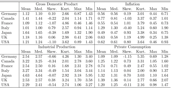
In general, the dispersion of forecast accuracy is quite large. Especially for forecasts of changes in industrial production and the forecasts for all variables in the U.K. the distance between the best and worst RMSEs is substantial. Most extreme examples are the forecasts for industrial production in Japan (2.8), the U.S. (2.2), Germany (2.1), and the U.K. (1.9), but also forecasts for less volatile variables such as real GDP growth in the U.K. (1.6), private consumption growth in the U.K. (1.4), or inflation in Italy (1.3). This first impression is further confirmed by the fact that the kurtosis of a sizable fraction of the distributions of RMSE across panelists considerably exceeds that of a normal distribution, indicating distributions of RMSEs with high density for extreme observations (Table 1). On average, kurtosis is highest for the forecasts for Germany (3.82), the U.K. (3.50), and for forecasts of the inflation rate (3.92). In addition, the distribution of forecast accuracy is considerably skewed in many cases, e.g., in case of inflation forecasts in Canada, France, or the U.K., and forecasts for real GDP growth in France or the U.S. However, we do not observe any systematic pattern of skewness. It seems to be a function neither of the different variables nor of the countries, and there is no tendency that forecasts are skewed more to the right or left.
Table 1. Descriptive Statistics on the Distribution of RMSEs across Panelists
Gross Domestic Product Inflation
Mean Med. Skew. Kurt. Max Min Mean Med. Skew. Kurt. Max Min Germany 1.12 1.10 0.10 2.66 0.87 1.43 0.56 0.56 0.19 3.01 0.44 0.71 Canada 1.41 1.44 -0.22 2.04 1.14 1.71 0.77 0.81 -1.03 3.37 0.37 1.01 France 1.09 1.12 -1.07 4.86 0.46 1.46 0.55 0.54 1.01 3.79 0.45 0.73 Italy 1.01 1.00 0.79 2.57 0.94 1.14 1.29 1.30 -0.40 5.24 0.60 1.90 Japan 1.64 1.65 -0.38 1.69 1.32 1.90 0.49 0.47 0.93 3.38 0.34 0.75 UK 1.18 1.16 0.06 2.98 0.41 2.06 0.63 0.58 1.19 4.99 0.25 1.38 USA 1.21 1.24 -1.10 3.62 0.89 1.43 0.62 0.61 0.80 3.64 0.46 0.93
Industrial Production Private Consumption
Mean Med. Skew. Kurt. Max Min Mean Med. Skew. Kurt. Max Min Germany 2.54 2.57 -0.66 4.26 1.30 3.40 1.09 1.09 -1.15 5.35 0.69 1.28 Canada 3.22 3.25 -0.34 2.01 2.78 3.60 1.25 1.22 0.73 3.31 1.05 1.60 France 2.54 2.50 0.16 1.68 2.31 2.78 0.74 0.71 0.49 2.47 0.55 1.02 Italy 3.27 3.34 -0.49 1.54 3.04 3.44 1.14 1.13 0.04 2.00 0.90 1.37 Japan 4.63 4.64 -0.07 2.92 3.18 5.95 1.32 1.31 0.70 3.03 1.10 1.64 UK 2.53 2.57 0.38 3.24 1.70 3.58 1.39 1.36 0.14 2.77 0.66 2.07 USA 2.29 2.41 -0.54 2.74 1.06 3.27 1.20 1.25 -0.11 2.16 0.98 1.47 Notes: All statistics refer to those RMSEs that correspond to the forecasts made with h= 12.
It would therefore be valuable to know, if there is any systematic pattern of (relative) forecast accuracy of a forecaster’s performance across variables. To answer this question,
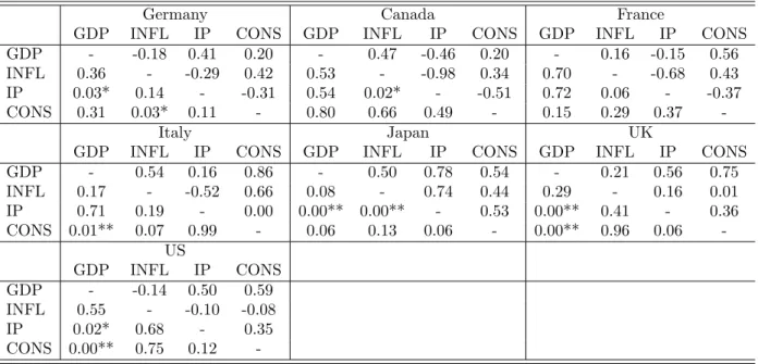
we show the correlations across panelists between any pairs of forecasts for two variables. High positive correlation coefficients would indicate that a forecaster who performs badly in terms of accuracy for one variable is also likely to perform badly for the other variable. Our results show that overall there are no high correlations between the forecast perfor-mance across variables–only about one quarter of the cross correlations are significantly different from zero (Table 2). One notable observation is, however, that 7 out of 10 sig-nificant correlations relate to cases involving the forecasts for real GDP growth. In all of the 7 cases, the correlation is significantly positive, indicating that more accurate GDP forecasts go together with more accurate forecasts for the other variables. This is, to some extent, not surprising, given that real GDP is the central variable in any business cycle forecasting model. This observation leads us to conclude that there is a tendency that those forecasters who have a suitable model for predicting real GDP growth also perform well in terms of forecast accuracy for other variables.
Table 2. Correlation of RMSEs across Variables
Germany Canada France
GDP INFL IP CONS GDP INFL IP CONS GDP INFL IP CONS GDP - -0.18 0.41 0.20 - 0.47 -0.46 0.20 - 0.16 -0.15 0.56 INFL 0.36 - -0.29 0.42 0.53 - -0.98 0.34 0.70 - -0.68 0.43 IP 0.03* 0.14 - -0.31 0.54 0.02* - -0.51 0.72 0.06 - -0.37 CONS 0.31 0.03* 0.11 - 0.80 0.66 0.49 - 0.15 0.29 0.37
-Italy Japan UK
GDP INFL IP CONS GDP INFL IP CONS GDP INFL IP CONS GDP - 0.54 0.16 0.86 - 0.50 0.78 0.54 - 0.21 0.56 0.75 INFL 0.17 - -0.52 0.66 0.08 - 0.74 0.44 0.29 - 0.16 0.01 IP 0.71 0.19 - 0.00 0.00** 0.00** - 0.53 0.00** 0.41 - 0.36 CONS 0.01** 0.07 0.99 - 0.06 0.13 0.06 - 0.00** 0.96 0.06 -US GDP INFL IP CONS GDP - -0.14 0.50 0.59 INFL 0.55 - -0.10 -0.08 IP 0.02* 0.68 - 0.35 CONS 0.00** 0.75 0.12
-Notes: Numbers above the diagonals indicate Pearson correlation coefficients computed across panelists; numbers below the diagonals denote the corresponding p-values for a test of zero-correlation. ∗ and∗∗
indicate significance on the 5%- and 1%-level. The correlations refer to those RMSEs corresponding to the forecasts made withh= 12.
4. Forecast Unbiasedness
4.1. Individual Forecast Unbiasedness. In this section, we present the empirical re-sults on the bias of the individual forecasts. For the estimation, we follow Davies and
Lahiri (1995) and deal with missing values by simply deleting the appropriate elements in the vectors of forecast errors eand the corresponding rows and columns in the covariance matrix Σ, respectively. The compressed matrices can be directly used to compute the estimates and corresponding standard errors (Blundell et al., 1992).
The analysis of the biases present in the individual forecasts reveal some notable dif-ferences across countries as well as variables. The results are summarized in Table 3.10 In general, most of the individual forecasts are unbiased. The overall performance is best for the inflation forecasts. There are very few biased forecasters for Canada, France, the U.K., and the U.S. Rather surprising is the good performance of inflation forecasts for Italy, which underwent a significant transition from a high to a low inflation regime during the early sample period. One might have imagined that forecasters adjusted only slowly to the new environment, causing forecasts to be biased upwards.
This expected behavior is similar to what can be observed for the inflation forecasts in the U.K., where inflation was also very high at the beginning of our sample period and then declined considerably to low levels in the mid 1990s. All but three panelists, who entered the sample rather late, overestimated inflation on average. After all, only 2 out of 30 did so significantly on a 95% confidence level.
A similar argument applies to the bias found in most of the forecasts for GDP growth in the European countries. Here the wide majority of forecasters overestimated growth on average. This phenomenon is most pronounced in Germany and Italy, but applies to a lesser extent also to France. The same is also true of the forecast for the growth of private consumption in Germany. Batchelor (2007) shows that this kind of bias can be inevitable in an environment of declining trend growth rates, since forecasters have to gradually realize the new trend.
A complex picture arises from the combination of forecasts for GDP growth and the growth of industrial production in the U.K. While forecasts for the former are generally unbiased, the results for the latter yield strong evidence for rejecting the hypothesis of unbiased forecasts; most panelist on average overestimate growth of industrial production
Table 3. Bias of Individual Forecasts
Gross Domestic Product Inflation
# obs # bias(+) # bias(-) mean var # obs # bias(+) # bias(-) mean var Germany 29 0 7 -0.49 0.021 30 0 0 -0.06 0.011 Canada 14 0 0 -0.27 0.020 14 0 3 -0.20 0.054 France 17 0 4 -0.40 0.016 17 0 2 -0.14 0.021 Italy 11 0 10 -0.61 0.002 11 0 0 0.20 0.010 Japan 13 0 0 -0.22 0.042 13 0 0 -0.13 0.011 UK 30 0 0 -0.25 0.025 30 0 2 -0.20 0.025 USA 22 0 0 0.23 0.023 22 0 1 -0.08 0.028
Industrial Production Private Consumption
# obs # bias(+) # bias(-) mean var # obs # bias(+) # bias(-) mean var Germany 28 0 0 -1.00 0.078 29 0 18 -0.52 0.039 Canada 4 0 0 -0.93 0.120 14 0 0 0.03 0.051 France 8 0 2 -0.98 0.093 17 0 0 -0.18 0.008 Italy 8 0 4 -1.53 0.048 11 0 0 -0.40 0.005 Japan 13 0 0 -1.26 0.089 13 0 0 -0.31 0.012 UK 28 0 22 -1.40 0.056 29 0 0 0.15 0.033 USA 21 0 0 -0.46 0.077 22 10 0 0.51 0.019 Notes: #obs indicates the number of individual panelists, #bias(+)/(−) indicate the number of them that provides significantly upward/downward biased forecasts. meanandvar indicate the mean and the variance of the biases across panelists.
by about 1 to 1.5 percentage points. This might reflect the fact that although the trend growth of overall output remained relatively constant over the sample, there was a shift in the structural composition of the economy in the U.K. from production-oriented sectors toward services – especially toward the financial sector – which had to be realized by the forecasters. A similar phenomenon can be observed when comparing forecasts on GDP growth for the U.S., which are generally unbiased, to forecasts for growth of private con-sumption in the U.S., which tend to underestimate concon-sumption growth. Again, it seems that it was difficult for a large number of panelists to anticipate the gradual decline in the saving rate of private households as well as to properly estimate additional consumption effects of huge increases in household wealth caused by the stock market boom of the late 1990s and the real estate boom from 2002 until the end of our sample.
In general, we can conclude that biased forecasts are apparently produced in times of structural shocks or gradual changes which have to be realized by the forecasters.11
On the contrary, forecasts seem to be generally unbiased for stable economies without large structural shocks. One example is Canada where the structure of the economy and the
11This source of bias in macroeconomic forecasts is also supported by results in Andolfatto et al. (2008),
who analyze the properties of artificial forecast generated within a standard dynamic stochastic general equilibrium model.
medium-term growth trend have not fundamentally changed since the introduction of inflation targeting in 1991. As a consequence, there are only 3 (out of 46) cases among all forecasts for the Canadian economy, in which the panelists produced biased forecasts.
5. Forecast Efficiency
5.1. Individual Forecast Efficiency. For testing weak efficiency of individual forecasts, we follow the literature (Clements, 1997, Harvey et al., 2001, Isiklar et al., 2006) by setting
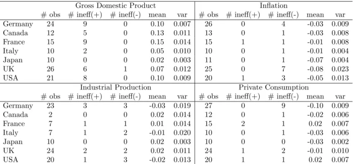
k in Eq. 9 equal to 1. Indeed, this makes sense since by the time a new revision is made, each forecaster knows about his most recent forecast revision. The results are summarized in Table 4.12
Our analysis of individual forecasts’ properties in terms of weak efficiency reveals an interesting contrast between the forecasts made for GDP growth and those made for the other variables under investigation in this paper. For the majority of forecasts on the growth of industrial production and private consumption as well as the inflation rate, we cannot reject the hypothesis of weakly efficient forecasts; only few series of forecasts show a significant correlation between successive forecast revisions. In those cases, the estimated coefficient is mostly negative, indicating that the forecasters in question tend to overreact to incoming news, i.e., at first, they overly revise their forecasts, undoing part of this revision during the next forecasting round.
In contrast, we find more evidence for deviations from weak efficiency for forecasts of GDP growth in all counties but Japan.13
The main difference is, however, that the estimated coefficients are positive in all but one of the significant cases. Accordingly, those forecasts for GDP growth that deviate from weak efficiency show a strong tendency toward forecast smoothing in general. This indicates that forecasters tend to process new information only slowly, which results in positively autocorrelated revisions.14
Gallo et al. (2002) find that forecasters tend to stick to their previous forecasts even when
12Again, detailed results for all individual panelists are available on request.
13The fact that we find weakly efficient forecasts for GDP growth in Japan is in contrast to the results
of Ashiya (2003), who analyzes the reaction of forecasters to news of GDP growth in a slightly different modeling framework and based on a different set of private sector forecasts; he concludes that forecasters tend to significantly overreact to new information.
14In psychology, this phenomenon is also known as conservatism (Phillips and Edwards, 1966, Edwards,
Table 4. Efficiency of Individual Forecasts
Gross Domestic Product Inflation
# obs # ineff(+) # ineff(-) mean var # obs # ineff(+) # ineff(-) mean var Germany 24 9 0 0.10 0.007 26 0 4 -0.03 0.009 Canada 12 5 0 0.13 0.011 13 0 1 -0.03 0.008 France 15 9 0 0.15 0.014 15 1 1 -0.01 0.008 Italy 10 2 0 0.05 0.010 10 0 1 -0.01 0.004 Japan 10 0 0 0.02 0.003 11 0 1 -0.07 0.004 UK 26 6 1 0.07 0.012 25 0 7 -0.08 0.023 USA 21 8 0 0.10 0.009 20 1 3 -0.05 0.013
Industrial Production Private Consumption
# obs # ineff(+) # ineff(-) mean var # obs # ineff(+) # ineff(-) mean var Germany 23 3 3 -0.03 0.019 27 0 9 -0.10 0.009 Canada 2 0 0 0.02 0.014 12 0 1 -0.02 0.006 France 7 1 1 0.01 0.014 15 2 1 0.02 0.007 Italy 7 1 2 -0.01 0.020 10 0 1 -0.03 0.006 Japan 10 0 0 0.02 0.003 10 0 0 -0.03 0.002 UK 24 2 2 0.02 0.011 24 1 2 -0.01 0.010 USA 20 1 3 -0.02 0.013 20 1 1 0.02 0.007 Note: #obsindicates the number of individual panelists,# ineff(+)/(-)the number of them that provides significantly weakly inefficient forecasts with positive/negative autocorrelated revisions. mean andvar
indicate the mean and the variance of the estimated autocorrelation coefficients across panelists.
controlling for the most recently observed average forecast and the dispersion of forecasts. Batchelor and Dua (1992) rationalize such forecasting behavior, noting that in reality forecasters might not have a single objective, which is to minimize the expected squared errors. Moreover, they are likely to take into account that their clients might “mistrust forecasters who make frequent [erratic] revisions to forecasts” (p. 179). The fact that the GDP growth forecast is usually the part of a comprehensive macroeconomic forecast report published by a forecaster, which is anticipated most by clients or the media, might result in just this behavior and make forecasters deviate most from their true expectations out of incentive and reputation considerations. This would explain why we find a strong tendency for forecast smoothing only for forecasts on GDP growth.
6. Conclusion
In this paper, we have analyzed individual macroeconomic forecasts for all G7 countries based on survey data from the Consensus Economics data set. We have shown the degree of heterogeneity across panelists with respect to forecast accuracy and tested whether the forecasts in the sample are unbiased and weakly efficient. The empirical results lead us to the following conclusions.
First, the dispersion of forecast accuracy is surprisingly high. Second, we observe that forecasters who perform well in terms of forecast accuracy for real GDP growth are also likely to perform well for other variables. Third, we find large difference in the performance of forecasters with respect to unbiasedness and efficiency across countries and different macroeconomic variables. Fourth, among the four kinds of forecasts analyzed, inflation forecasts perform best in terms of unbiasedness. Fifth, forecasters, on average, seem to smooth their GDP forecasts more heavily relative to the other macroeconomic forecasts they make. Sixth and last, forecasts tend to be biased in situations where forecasters have to realize large structural shocks or gradual changes in the trend of a variable. As a consequence, if a sizeable fraction of panelists produce biased forecasts for a variable, then virtually all of them are biased in the same direction, i.e., biases are not uncorrelated across panelists.
There are several dimensions along which this research could be expanded in the future. For simplicity, we have assumed that the variance of the macroeconomic shocks (λt,h) as
well as the variance of the forecaster-specific error component (i,t,h) decay linearly if h
goes to 1. First, more general functional forms could be developed in the future to better match the data. Second, as soon as a sufficient number of longer time series become available for forecasters of individual forecasts, one could implement the estimation of horizon-specific bias, which would be more attractive from a theoretical point of view. Currently, however, the time dimension of the data set is too small, that is, for most of the panelists the estimates would be based on fewer than ten observations. Finally, taking into account correlations across countries – as Isiklar et al. (2006) do in their analysis of consensus forecasts – would clearly be desirable, given the high impact that international shocks potentially have on the size of forecast errors. However, this would require immense computational power for the estimation of the covariance matrices.
References
Ager, P., Kappler, M., Osterloh, S., 2009. The accuracy and efficiency of the consensus forecasts: A further application and extension of the pooled approach. International Journal of Forecasting 25 (1), 167–181.
Andolfatto, D., Hendry, S., Moran, K., 2008. Are inflation expectations rational? Journal of Monetary Economics 55 (2), 406–422.
Ashiya, M., 2003. Testing the rationality of Japanese GDP forecasts: The sign of forecast revision matters. Journal of Economic Behavior & Organization 50, 263–269.
Ball, R. J., 1962. The prediction of wage-rate changes in the United Kingdom economy 1957-60. Economic Journal 72, 27–44.
Batchelor, R., 2001. How useful are the forecasts of intergovernmental agencies? The IMF and OECD versus the consensus. Applied Economics 33, 225–235.
Batchelor, R., 2007. Bias in macroeconomic forecasts. International Journal of Forecasting 23, 189–203.
Batchelor, R., Dua, P., 1990. Forecaster ideology, forecasting technique, and the accuracy of economic forecasts. International Journal of Forecasting 6, 3–10.
Batchelor, R., Dua, P., 1992. Conservatism and consensus-seeking among economic fore-casters. Journal of Forecasting 11, 169–181.
Blundell, R., Bond, S., Devereux, M., Schiantarelli, F., 1992. Investment and Tobin’s Q: Evidence from company panel data. Journal of Econometrics 51, 233–257.
Boero, G., Smith, J., Wallis, K. F., 2008a. Evaluating a three-dimensional panel of point forecasts: The Bank of England Survey of External Forecasters. International Journal of Forecasting 24, 354–367.
Boero, G., Smith, J., Wallis, K. F., 2008b. Here is the news: Forecast revisions in the Bank of England Survey of External Forecasters. National Institute Economic Review 203, 68–77.
Bowles, C., Friz, R., Genre, V., Kenny, G., Meyler, A., Rautanen, T., 2007. The ECB sur-vey of professional forecasters (SPF). Review after eight years’ experience. Occasional paper series 59, European Central Bank.
Capistran, C., Timmermann, A., October 2006. Disagreement and biases in inflation expectations, mimeo.
Clements, M. P., 1997. Evaluating the rationality of fixed-event forecasts. Journal of Forecasting 16, 225–239.
Clements, M. P., Joutz, F., Stekler, H. O., 2007. An evaluation of the forecasts of the Federal Reserve: A pooled approach. Journal of Applied Econometrics 22 (1), 121–136. Croushore, D., 2006. Forecasting with real-time macroeconomic data. In: Elliott, G., Granger, C. W., Timmermann, A. (Eds.), Handbook of Economic Forecasting Volume 1. North-Holland, Amsterdam.
Davies, A., Lahiri, K., 1995. A new framework for analysing survey forecasts using three-dimensional panel data. Journal of Econometrics 68, 205–227.
Dovern, J., Fritsche, U., Slacalek, J., 2009. Disagreement among forecasters in G7 coun-tries. Working Paper 1082, European Central Bank.
Dovern, J., Weisser, J., 2008. Are the really rational? Assessing professional macro-economic forecasts from the G7 countries. Kiel Working Paper 1447, The Kiel Institute for the World Economy.
Edwards, W., 1968. Conservatism in human information processing. In: Kleinmuntz, B. (Ed.), Formal Representations of Human Judgements. Wiley, New York.
Figlewski, S., Wachtel, P., 1981. The formation of inflationary expectations. Review of Economics and Statistics 63, 1–10.
Gallo, G. M., Granger, C. W., Jeon, Y., 2002. Copycats and common swings: The impact of the use of forecasts in information sets. IMF Staff Papers 49, 4–21.
Harvey, D. I., Leybourne, S. J., Newbold, P., 2001. Analysis of a panel of UK macroeco-nomic forecasts. Econometrics Journal 4, 37–55.
Isiklar, G., Lahiri, K., Loungani, P., 2006. How quickly do forecasters incorporate news? Evidence from cross-country surveys. Journal of Applied Econometrics 21, 703–725. Keane, M. P., Runkle, D. E., 1990. Testing the rationality of price forecasts: New evidence
from panel data. American Economic Review 80, 714–735.
Lahiri, K., Sheng, X., 2008. Evolution of forecast disagreement in a Bayesian learning model. Journal of Econometrics 144 (2), 325–340.
Laster, D., Bennett, P., Geoum, I. S., 1999. Rational bias in macroeconomic forecasts. The Quarterley Journal of Economics, 293–318.
Loungani, P., 2001. How accurate are private sector forecasts? Cross-country evidence from consensus forecasts of output growth. International Journal of Forecasting 17, 419–432.
Mincer, J., Zarnowitz, V., 1969. The evaluation of economic forecasts. In: Mincer, J. (Ed.), Economic Forecasts and Expectations. National Bureau of Economic Research, New York.
Nordhaus, W. D., 1987. Forecasting efficiency concepts and applications. Review of Eco-nomics and Statistics 69, 667–674.
Pesaran, M. H., Weale, M., 2006. Survey expectations. In: Elliott, G., Granger, C. W., Timmermann, A. (Eds.), Handbook of Economic Forecasting Volume 1. North-Holland, Amsterdam.
Phillips, L. D., Edwards, W., 1966. Conservatism in a simple probaility inference task. Journal of Experimental Psychology 72, 346–357.
Stege, C., 1989. Zur Beurteilung der Prognoset¨atigkeit der “f¨uhrenden Wirtschaftswis-senschaftlichen Forschungsinstitute” in der Bundesrepublik Deutschland. Verlag Dr. Kovac.
Stekler, H. O., 2002. The rationality and efficiency of individuals’ forecasts. In: Clements, M. P., Hendry, D. F. (Eds.), A Companion to Economic Forecasting. Blackwell Pub-lishers Inc., Oxford.
Timmermann, A., 2007. An evaluation of the World Economic Outlook forecasts. IMF Staff Papers 54 (1), 1–33.