Model compression methods for convolutional neural networks

Model compression methods for

convolutional neural networks

Faculty of Information Technology and Communication Sciences (ITC) Master’s thesis November 2019

Henri Lunnikivi: Model compression methods for convolutional neural networks Master’s thesis

Tampere University

Master’s Degree Programme in Information Technology November 2019

Deep learning has been found to be an effective solution to many problems in the field of computer vision. Convolutional networks have been a particularly successful model for computer vision. Convolutional neural networks extract feature maps from an image, then use the feature maps to determine to which of the preset categories the image belongs. Convolutional neural networks can be trained on a powerful machine, and then deployed onto a target device for inference. Computing inference has become feasible on mobile phones and IoT edge devices. However, these devices come with constraints like reduced processing resources, smaller memory caches, decreased memory bandwidth. To make computing inference practical on these devices, the effectiveness of various model compression methods is evaluated quantitatively. Methods are evaluated by applying them on a simple convolutional neural network for optical vehicle classification. Convolutional layers are separated into component vectors for a reduction in inference time on CPU, GPU, and an embedded target. Fully connected layers are pruned and retuned in combination with regularization and dropout. Pruned layers are compressed using a sparse matrix format. All optimizations are tested on three platforms with varying capabilities. Separation of convolutional layers improves latency of the whole model by 3.00×

on a CPU platform. Using a sparse format on a pruned model with a large fully connected layer improves latency of the whole model by 2.01× on desktop with a GPU and by 1.82× on the embedded platform. On average, pruning the model allows 39.1× reduction in total model size while causing a 1.67 %-point reduction in accuracy, when dropout is used to control overfitting. This allows for a vehicle classifier to fit in 180 kB of memory with reasonable reduction in accuracy.

Keywords: CNN, cross-platform, deep learning, dropout, GPGPU, Mali, master of science thesis, model compression, neural networks, OpenCL, pruning, Rust, separable convolutions, supervised learning.

The originality of this thesis has been checked using the Turnitin Originality Check service.

Henri Lunnikivi: Konvoluutioneuroverkkojen mallinpakkausmenetelmien arviointi Diplomity¨o

Tampereen yliopisto

Tietotekniikan DI-tutkinto-ohjelma Marraskuu 2019

Syv¨aoppimisen on todettu olevan hyv¨a ratkaisu moniin konen¨a¨on ongelmiin. Ko-nen¨a¨on sovelluksissa erityisen menestyksekk¨a¨asti k¨aytetyt konvoluutioneuroverkot yksinkertaistavat laskentaa erottelemalla kuvasta korkean tason piirrekarttoja (engl. feature map). Konvoluutioneuroverkkoja voidaan kouluttaa tehokkaalla laitteistolla, josta mallin painokertoimet voidaan ottaa k¨aytt¨o¨on kohdelaitteelle. Mallin k¨aytt¨amis-est¨a on tullut mahdollista matkapuhelimissa ja Internet-reunalaitteissa. N¨am¨a lait-teet ovat kuitenkin usein monella tavalla rajoittuneita: v¨ahemm¨an laskentakapa-siteettia, pienemm¨at v¨alimuistit ja v¨ahemm¨an erilaisten muistien v¨alist¨a kaistan-leveytt¨a. Jotta mallin k¨aytt¨amisest¨a voitaisiin tehd¨a k¨ayt¨ann¨ollisemp¨a¨a t¨allaisilla laitteilla, erilaisten mallinpakkausmenetelmien tehokkuutta arvioidaan kvantitatiivis-esti. Ty¨oss¨a menetelmi¨a arvioidaan k¨aytt¨aen niit¨a yksinkertaiseen konvoluutioneu-roverkkoon, joka luokittelee ajoneuvoja optisesti. Konvoluutiokerrokset optimoidaan separoimalla ne pohjavektoreiksi, jotta mallin k¨aytt¨aminen olisi laskennallisesti yksinkertaisempaa. T¨aysin kytkettyjen kerrosten v¨ahiten merkityksellisi¨a painok-ertoimia karsitaan regularisoinnin (engl. regularization) ja dropout-menetelmien avulla. Karsitut kerrokset pakataan harvaan matriisimuotoon. Optimoituja verkkoja testataan p¨oyt¨atietokoneen suorittimella, grafiikkasuorittimella ja tyypillisell¨a su-lautetulla laskentaj¨arjestelm¨all¨a. Konvoluutioiden separointi nopeuttaa koko mallin suoritusta 3-kertaisesti tavallisella suorittimella. Karsitut mallit ja harva matri-isimuoto nopeuttavat mallin suoritusta 2,01-kertaisesti kun konvoluutiot voidaan ajaa grafiikkasuorittimella. Vastaava nopeutus sulautetulla laskentaj¨arjestelm¨all¨a on 1,82-kertainen. Mallin karsiminen v¨ahent¨a¨a mallin kokonaismuistivaatimusta 39,1-kertaisesti, aiheuttaen noin 1,67 %-yksik¨on menetyksen tarkkuudessa, kun k¨aytet¨a¨an dropout-menetelm¨a¨a ylisovittumisen (engl. overfitting) est¨amiseen. T¨am¨a mahdollis-taa ajoneuvoluokittelijan sovittamisen 180 kilotavuun muistia.

Avainsanat: diplomity¨o, dropout, GPGPU, konvoluutioneuroverkot, Mali, mallinpakkaus, neuroverkot, OpenCL, pruning, Rust, separoituvat konvoluutiot, syv¨aoppiminen, valvottu oppiminen.

1 Introduction . . . 1

1.1 Deep neural networks and image recognition . . . 2

1.2 Deep models with resource-constraints . . . 4

1.3 Separable convolutions and sparse layers . . . 5

2 Convolutional neural networks and model compression . . . 6

2.1 The structure of a convolutional neural network . . . 7

2.1.1 Fully connected layer . . . 8

2.1.2 Convolutional layer . . . 10

2.1.3 Rectifier linear unit . . . 11

2.1.4 Softmax . . . 13

2.2 Model training and the pruning process . . . 13

2.2.1 Calculating training loss . . . 14

2.2.2 Backpropagation . . . 15 2.2.3 Gradient descent . . . 17 2.2.4 Regularization . . . 17 2.3 Proposed optimizations . . . 19 2.3.1 Weights pruning . . . 19 2.3.2 Sparse models . . . 20 2.3.3 Separable convolutions . . . 20 3 Implementation of optimizations . . . 23

3.1 Use case: a convolutional network for car type recognition . . . 23

3.2 Implementation of training . . . 25

3.2.1 Pruning . . . 25

3.2.2 Assessment of model accuracy and overfitting . . . 26

3.3 Inference optimizations . . . 26

3.3.1 Sparse matrix multiplication . . . 27

3.3.2 Separable convolutions . . . 30

4 Measurements . . . 31

4.1 Data collection . . . 31

4.1.1 Threshold pruning . . . 33

4.1.2 L2 pruning . . . 33

4.1.3 L2 pruning with 50 % dropout . . . 35

4.1.4 Performance measurements . . . 36

4.2 Analysis of results . . . 39

4.2.4 Combining pruning and separable convolutions . . . 42 4.2.5 Reliability of results . . . 42 4.3 Summary of findings . . . 43 5 Conclusions . . . 44 5.1 Discussion . . . 44 5.2 Recommendation . . . 45 5.3 Future work . . . 45 References . . . 48

Adam Adaptive moment estimation algorithm for gradient descent AI Artificial intelligence

ASIC Application specific integrated circuit AVX Advanced vector extensions

BLAS Basic linear algebra subroutine CNN Convolutional neural network CPU Central processing unit CRS Compressed row storage CSB Compressed sparse blocks DNN Deep neural network

DRAM Dynamic random-access memory FMA Fused multiply-add

FPGA Field-programmable gate array GAN General adversarial network GEMM General matrix multiply

GPGPU General-purpose computing on graphics processing units GPP General purpose processor

GPU Graphics processing unit MAC Multiplier-accumulator MLP Multilayer perceptron MSE Mean squared error ReLU Rectifier linear unit

SGD Stochastic gradient descent SIMD Single instruction, multiple data SIMT Single instruction, multiple threads SRAM Static random-access memory SSE Streaming SIMD extension SVM Support vector machine TPU Tensor Processing Unit

VCN A convolutional neural network for vehicle classification [15] by Huttunen et al.

nnz Non-zero

fN N-bit floating-point number (eg. float f32, double f64) iN N-bit signed fixed-point integer (eg. signed char, short, int) uN N-bit unsigned fixed-point integer (eg. unsigned char) N The set of all natural numbers n ∈[1,∞[

Z The set of all integers.

1 Introduction

Deep learning is becoming pervasive as a solution to problems in the field of computer vision. In 2012, Cire¸san et al. [6] reported reaching and exceeding of human level performance on state of the art computer vision benchmarks. Soon after, Krizhevsky’s

convolutional neural network [20] classified the 1000-category ImageNet database of images with unprecedented accuracy. They achieved this level of accuracy by using a significantly more efficient training procedure that enabled them to fit a large model to the 1.2 million training examples of the huge ImageNet database. The best modern deep learning models, based on the convolutional neural network archetype, are able to create photorealistic images of people [18] or transform hand-drawn style guide images into synthesized photorealistic sceneries [26].

Research on convolutional neural networks and their derivatives has produced impressive results. The number of applications for convolutional neural networks and other deep learning models has increased steadily. The wealth of applicability is making deep learning pervasive, and there is a growing interest in how to deploy deep learning models on mobile phones, embedded devices, wearables, and in other applications of edge computing [1, 15].

As AI becomes pervasive, the requirements to supporting infrastructure increase as well. Pushing location of computing towards the end-user helps reduce total power consumption and increase privacy. However, deep learning and edge computing is a difficult combination. Resource constraints include: limited memory size and bandwidth, limited processing power and requirements for efficient usage of hardware. Simpler processors andapplication specific integrated circuits (ASICs) are often used instead of general purpose processors. In the past, running a deep learning model on an edge device has seemed like a tall order. In recent years, there has been plenty of research into compressing models. An older state-of-the-art deep model like AlexNet [20] used to have 60 million parameters, while recent cutting edge networks like MobileNetV21 _{[28] have only a little more than 2 million parameters for a similar or}

better accuracy. Another recent space-optimized variant, SqueezeNet, only has 1.2 million parameters, resulting in a<500 kB model size [16].

For edge computing, reducing resource usage of deep learning models also results in less communication between devices, which results in less total power used and better bandwidth usage. Enabling a model to run on an edge device also mitigates the privacy problems inherent with the very common practice of server-offloading, where a picture taken on a cell phone might be sent to a server for processing. Moving

1_{open-sourced and available as part of}

TensorFlow-Slim Image Classification Library

the processing onto a user’s phone or an intermediate edge device lessens problems caused by server-offloading. Additionally, it makes it easier for a user to be aware of where their data has gone.

The particular constraints of edge platforms create a need for particular techniques and processes. There is a need for models that are smaller, require less power, and that enable computation on the device instead of server-offloading. Enabling creation of models like this makes it possible to apply deep learning models on a wider range of platforms for cheaper and more securely than before.

The aim of this work is to evaluate the effects, results and platform applicability of some recent techniques in creating smaller and more efficient models. The main methods evaluated are cross-platform model compression and computational approximations.

1.1

Deep neural networks and image recognition

The neural network is a basic model structure of deep learning. A neural network comprises interconnected weights, or parameters, that transform the inputs in a series of layers. A properly trained network with enough input data can infer classes or attributes from unseen inputs. An instance of a simple deep neural network (DNN) is the multilayer perceptron (MLP). A MLP takes selected features as a vector of inputs. Inputs are then multiplied in chained fully connected hidden layers and a nonlinearity for each layer. The role of fully connected layers is to apply a weight to each of the inputs, and the role of the nonlinearities is to simulate an activation of a neuron. Fully connected layers are often implemented as plain matrix multiplications, while there are multiple popular implementations of different activation functions. To summarize, the inputs to the network are progressively multiplied with matrices and then activated in a predefined structure of layers.

The many parameters of a network can be algorithmically stabilized such that the resultant model can correctly classify input data it has never seen before. This is called training of weights. Training can be done by ”showing” the network carefully selected and correctly labeled input data, and adjusting the weights towards the least error with a gradient descent algorithm. In addition to the parameters, a network is defined by its hyperparameters. The typical hyperparameters of a network are the number of layers and the cardinality of each layer. The first layer starts the transformation of the input data, and the last layer provides a representation of the desired outputs.

The creation and operation of a neural network can thus be coarsely divided into two phases: training and inference. The training phase involves the use of a massive set of training data to estimate the correct parameters for the network. Training until the network stops learning (ie. convergence) can often take hours, days

or weeks depending on the size of the model and the availability of computational resources. In inference, the deployed network is making predictions on data it has never seen before, and the training data set needs not be present on the inference device. Inference is a real-time application. Real-time applications are often latency sensitive and constrained by available resources on the real-world platforms that need to be doing the inference. While training is mostly done on a high performance computer, inference might be run on a small edge device. Examples of devices that might be running inference would be an end user’s cell phone, or an integrated system like a security camera.

Hardware manufacturers have risen to the occasion by developing various hardware solutions to accelerating computations for machine learning, both for server-side and edge computing. At Google I/O, in 2016, Google announced its Tensor Processing Unit (TPU), which had already been in use in their data centers. A TPU resembles a GPU in its ability to do high volumes computation power efficiently but lacks rasterization and texture mapping capabilities. In 2018, Google announced the Edge TPU - a power efficient ASIC for machine learning in edge computing. All of the optimizations measured on a GPU in this thesis should also translate to comparable TPUs with similar effects on performance, possibly with further reductions in power consumption. Other notable machine learning manufacturers include Intel Movidius2

which produces special hardware for computer vision, and Huawei with their Kirin3

-family of SoC chipsets, which are oriented for mobile AI.

The convolutional neural network (CNN) is a special case of a deep neural network, with layers of adaptive feature extractors before the fully connected layers. CNNs have held the title of being the best adaptive image recognizer since 2011, when Cire¸san et al. used CUDA to accelerate the training of a general, fully parameterizable convolutional network on a GPU platform. That implementation used maxpooling and gradient descent on a GPU to achieve best published results on object classification benchmarks of that time (NORB, CIFAR10, MNIST). [5]

The bar for the state-of-the-art of convolutional neural networks was again raised in 2012 by Alex Krizhevsky’s AlexNet [20]. His work enabled quick training of CNNs on very large datasets. This was achieved by speeding up network training via swap-ping the commonly used nonlinearity functionf(x) = tanh(x) for a nonsaturating nonlinearity called ReLU, and then by training the network using a GPU. ReLU is defined simply as R(x) = max(0, x) and it was first applied in signal processing by Hahnloser et al. in 2000 [9]. ReLU and its gradient are easy to compute on a GPU. This technique has been found to consistently reduce model training times by at least a factor of 2−6×. Additionally, they effectively reduced model overfitting by

2_{https://www.movidius.com/}

use of a technique calleddropout, where half of the model parameters are randomly selected for temporary deactivation during training.

1.2

Deep models with resource-constraints

Deep learning models have come a long way in ease of computing. Creating and training a model with sufficient predictive power used to be difficult, but is now practical. While the process of training an effective computational model is still a task better fit for specialized, high-capacity hardware, the inferring models have become small. The size reduction of models has proven it possible [21] to fit a model on an embedded device, with constraints on memory bandwidth and processing power. In 2016, Iandola et al. introduced SqueezeNet [16], that reaches AlexNet level accuracy on ImageNet with 50×less parameters. SqueezeNet can also be compressed into the size of 0.5 MB, which is 510×smaller than AlexNet. Running these networks on smaller devices, ASICs and FPGAs is now viable.

Reducing model size has many advantages. Memory access on small devices is generally energy intensive. Han et al. indicate that in a neural network, the energy use per operation is most dependent on the type of memory access: 5 pJ for on-chip SRAM and 640 pJ on off-chip DRAM [11]. There is a 100-fold difference in using a register w.r.t. using the main memory. Reducing the size of the network is generally effective in reducing the total energy cost of the network by moving the computation closer to the processor.

Another advantage of small model size is when a model is trained in a distributed environment, where servers need to communicate less [16]. Lane and Bhattacharya discuss that many of the current models running on smaller devices also offload the inference to an external server [1]. This causes a privacy issue where unnecessary data, such as the pictures that a cell phone user takes, leak further away from the device where they are needed. Not requiring cloud offloading for inference alleviates these privacy concerns.

Smaller model size implies that less data need to move between circuits and between devices. For the current processor architectures, this means that a smaller network layer might fit into a different kind of a memory or a smaller cache that is closer to the computation device doing the work. Moving less data between devices is also obviously beneficial to reduce network load and delays in real-time systems. There has been continuing research interest in reducing the size of deep models. A recent study [10] by Han, Mao and Dally has been able to reduce the memory footprint of AlexNet by 35× and the memory footprint of the VGG-16 by 49×, both with only a very slight reduction in accuracy. This was achieved via pruning of low-relevance weights, trained quantization and Huffman coding.

SparseSep to reduce the memory footprint of a CNN consisting of both a notable amount of convolutional layers and fully connected layers. In SparseSep, the idea is to compress the fully connected layers via use of sparse matrices and the convolution layers via separation of the kernels into vectors. Both techniques involve insertion of a new layer to get a reduction in total number of computations. The techniques produce a minor loss in accuracy, but they claim to use principled methods that avoid specializing the original model to recognize a smaller set of activities/contexts. They were able to reduce the memory footprint of some commonly used deep neural networks by 11.3×on average and get the networks to run 13.3×faster on platforms like Qualcomm Snapdragon 400, ARM Cortex M0 and M3, and Nvidia Tegra K1.

1.3

Separable convolutions and sparse layers

Effective compression of convolutional neural networks requires strategies that are able to reduce the size of both convolutional and fully connected layers. Model pruning is a method of removing low impact parameters and has been previously used effectively in model compression [10, 34], though it has been shown to be mostly effective on the fully connected layers, and less so on convolutional layers.

Combining the model pruning approach with an orthogonal approach for reducing the size of the convolutional layers is an effective way to gain good total model compression. An effective way to reduce the cost of the convolutional layers has been introduced by Jaderberg et al. [17]. They exploit the redundancy between different filters by decomposing the convolution into a horizontal and a vertical convolutional vector.

In this study, the effects of several recent inference optimization techniques are investigated in the context of a small CNN [15]. This CNN classifies images into four classes of vehicles. The network will be introduced in detail in Chapter 3. The performance characteristics of the compressed layers are empirically mapped for three different devices: a desktop computer with a graphical processor, a multithreading Intel CPU and a representative embedded computer.

2 Convolutional neural networks and model

compression

Making a small MLP capable of making predictions on images is nigh impossible due to the large size of image files. Multiplying the pixels of an image taken on a multi-megapixel camera with a weights matrix costs unfeasibly high amounts of computing power. Fortunately, much smaller images, like a 128×128 pixels RGB image, usually contain enough information for a computer to make predictions on. However, this is still too large to enable training a MLP and another approach is required.

Prior to training, MLP has no presumption of any correlation between the parameters of the input layer. In a real world image, the close-together pixels are strongly correlated. A more macroscopic feature of the image might have significance regardless of its position in the image. Given enough training data, a MLP may learn to account for this, but it is computationally very costly. The other option is to build these types of correlations into the model via use of techniques called local receptive fields, weight sharing and subsampling (Chapter 2). This is what makes up a convolutional neural network (CNN). [2, pp. 267-269]

Convolutional neural networks solve the problem of extracting macroscopic features from the image instead of treating each input pixel as a feature. This has allowed models to have much less parameters, e.g. one 3×3 kernel of parameters per feature instead of one for each combination of one pixel and one hidden layer node.

The convolutional neural network (CNN) is a DNN that is widely applied in image recognition tasks [2, p. 267], and has in fact been the state-of-the-art model architecture of image recognition since the implementation by Cire¸san et al. [5]. It differs from a MLP in the inclusion of one or more convolutional layers at the start of the network. To understand the purpose of including the convolutional layers, the difference to a MLP is explained next.

Prior to training, a DNN does not assume any correlation between the parameters of the input layer, though it may learn it with enough input data. A convolutional neural network uses the intrinsic properties of images to extract relevant information before the fully connected layers. This is achieved by leveraging the fact that the close-by pixels of a real-world photo are more related to each other than distant pixels. Convolutional layers extract local features into feature maps using local receptive fields and weight sharing (2.1.2 Convolutional layer). Stacking more than one convolutional layer makes it possible to extract higher-order features. Convolutional layers are often paired with subsampling layers that effectively reduce the amount of

data in the pipeline and make the network less sensitive to small input translations. [2, pp. 267-269]

An illustration of a convolutional neural network is presented in Figure 2.1.

Figure 2.1 An illustration of a CNN [32].

As seen in Figure 2.1, features get extracted with convolutions from an image into feature maps. These feature maps get subsampled into smaller feature maps. From those smaller feature maps, higher order features are extracted and again subsampled. The final layer of feature maps gets fed into one or more fully connected layers that produce the final output.

2.1

The structure of a convolutional neural network

Convolutional neural networks are essentially a stack of linear algebra, organized into layers. This section describes the different layer types and the non-linear activation functions used for post-processing layer outputs.

A convolutional neural network predicts the class of an input image from a number of pre-defined categories. It does so by passing the input image through a series of specifically weighted layer transformations in the form of convolutions and matrix multiplications. Transforming an input with a well-selected set of weights produces the right class label for a given input image. Obtaining well-selected weights for the layer transformations is called training of the model. The particulars of training are further explained in Section 2.2.

When a CNN makes a class prediction (i.e. inference), inputs are transformed through a series of layers. Each layer has a hyper-dimensional weights matrix - i.e. a tensor that the input gets multiplied with. The structure of a layer transformation generally matches the following template:

1. an input tensor, ...

2. multiplied or convolved with a weights tensor, ...

4. producing an output tensor.

The exact shape and function of each of the parts varies between different layers. Weights might function like a filter in a convolutional layer, or as a simple weighting matrix for a set of input neurons in a fully connected layer. In post-processing, the output may be aggregated to a reduced size, and/or an activation function may be applied to transform each element in the output to otherwise enhance the capabilities of the network. Finally, the outputs are propagated to the next hidden layer, or the final output probabilities.

The linear algebra needed for inference includes cross-correlation for convolution, matrix multiplication for fully connected layers and an activation function for the nonlinearities. In convolutional layers, features are extracted from the input image using local receptive fields (i.e. filters) that multiply-add or convolve each pixel in the input. This produces a feature map that is subsampled to a smaller feature map that makes it more invariant to small translations in input data. Reduced-size feature maps from subsampling are fed into fully connected layers. In a multiclass image classification application, the last layer would usually be a fully connected layer, with a softmax nonlinear function to convert numbers into action probabilities matching with each output class. [2, p. 267-269]

The simplest part of a CNN, a commonality with the MLP, is the fully connected layer.

2.1.1

Fully connected layer

The fully connected layer is the basic building block and the defining factor of most contemporary neural networks. A model consisting only of fully connected layers and activations is called a multilayer perceptron or a feed-forward neural network. In their 2006 book, Bishop et al. described it as having been proven to be the network type of greatest practical value in pattern recognition [2, p. 226]. The modern convolutional neural network such as the one used by Krizhevsky et al. [20] still uses this layer type to correlate image features and outputs.

A fully connected layer, put simply, is a matrix multiplication between well-selec-ted parameters and values of input neurons, producing the values of output neurons

~zl with a bias weight~b sometimes added to each output neuron.1 These outputs

become activations after being activated by the activation function. The vector formed by the activations of neurons in one layer is denoted with~al. Obviously, what

follows is that the activations of neurons in any preceding layer are called~al−1, and 1_{Mathematical descriptions about multilayer perceptrons and backpropagation in this chapter}

the neurons in the following layer are called~al+1. The structure of a fully connected

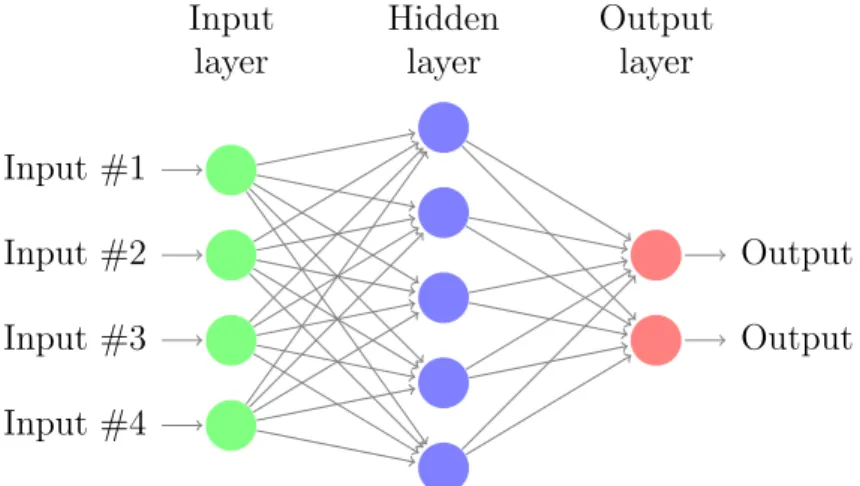
layer in the context of a simple neural network is illustrated in Figure 2.2.

Input #1 Input #2 Input #3 Input #4 Output Output Hidden layer Input layer Output layer

Figure 2.2 An illustration of a simple feed-forward neural network with one hidden layer. [8]

In a fully connected layer, every neuron is connected to every neuron in the previous layer multiplied by a weight. Mathematically, this is matrix multiplication between the activations of the previous layer~al−1 ∈RM×1, whereM is the number of

neurons in the previous layer, and the weights matrix Wl ∈RN×M, where N is the

number of neurons in the current layer. Additionally, there can be one bias variable

bl summed to each output neuron, though the network described later in this thesis

manages without. This calculation produces outputzl= Wlal−1+bl∈RN×1. Finally,

an activation function is applied to the output. The rectifier function (denoted byR) is used in all layers except the last one. The rectifier functionR is better explained later in Subsection 2.1.3. The activations of a given layer are defined in terms of the activations in the previous layer as follows:

~al =R(Wl~al−1+~bl). (1.1)

The network described later in this thesis (Chapter 3) contains no biases, so the expression for the fully connected layer simplifies to:

~al =R(Wl~al−1). (1.2)

In a MLP, these fully connected layers are chained, and the result of the final layer~aL can be calculated recursively based on Equation 1.2. Executing this part of

the algorithm on a computer is called a forward pass. A forward pass is required for both the first training pass, and later when the model is deployed, during inference. The matrix multiplications of the fully connected layers can be efficiently computed on most kinds of contemporary hardware by using highly optimized general matrix

multiplication implementations (GEMM), while applying the rectifier function is very efficient on all kinds of processors.

2.1.2

Convolutional layer

Fully connected layers and non-linearities can be used to represent the solution to any problem space, though this is often computationally expensive and redundant. The common solution to this problem in the domain of image recognition is to first extract features from the input data using convolutional layers.

The convolutional layer is a solution to the inability of the fully connected layer to correlate spatial locality, with the benefit of drastic reduction in total computation and number of weights required. Correlating spatial locality is achieved via use of local receptive fields, weight sharing and subsampling. These techniques substantially reduce the number of parameters in the network when compared to a fully connected layer. [2, p. 269]

A convolutional layer processes an image into a set ofF feature maps byconvolving

the image withF weights kernels. Each feature map is produced by convolving the respective weights kernel with each overlapping, kernel-sized neighborhood of input pixels. Each of the kernels essentially detects one pattern or feature within the input image in all positions of the image. Multiple chained convolutional layers detect higher-order features. [2]

In the network under optimization (explained later in Section 3.1), there is a downsampling layer after each convolution. The subsampling layer takes as input all nonoverlapping rectangles of the feature map and picks the highest value as output. A 2×2 max pooling layer would then produce a half-sized version of the feature map. Chaining convolution layers with subsampling layers increases the degree of invariance of features to minor input transformations [2].

The algorithm for a convolutional layer is, in principle, similar to a filter in an image processing program. In the algorithm for a monochrome image, a weighted, constant-sized, 2D filter is multiplied over each input pixel neighborhood. Then the

products are summed, which produces a single output pixel. This repeats for every input pixel, producing a 2D set of pixels known as the feature map. This process repeats for a number of times for a number of different filter weights, thus producing a number of different feature maps. The multicolored RGB version of this algorithm changes only in that the filters are 3-dimensional, where the last dimension is the color. Each 3D neighborhood still produces one singular output pixel per feature map because the products for each color are finally summed.

Given a specific hard-coded kernel and convolving it over an image, a variety of effects can be produced, as seen in Figure 2.3. In model training, this effect is turned around to train the weights of the convolutions such that they produce maps

of trainable features.

Convolution in machine learning is almost always implemented ascross-correlation. Using the notation introduced in Subsection 2.1.1, 2-D cross-correlation between a monochrome input image of (i, j)∈ W ×H and the (u, v)∈K ×K kernel of one feature map is expressed as:

~zl,i,j =Wl? ~al−1 , k X u=−k k X v=−k Wl,u,v~al−1,i+u,j+v.

Here,?is used to denote cross-correlation andk = _bK

2cis the radius of the kernel.

The inputs to a convolution usually have multiple channels C (eg. in RGB, C = 3), and multiple features are detected usingF filters. Adding in c_∈NC channels and

f _∈NF filters and feature maps, the final equation for 3-D cross-correlation is defined

as ~zl,f,i,j =Wl? ~al−1 , C X c=1 k X u=−k k X v=−k Wl,f,u,v~al−1,i+u,j+v. (2.2)

A plain convolution innately produces a slightly smaller feature map in relation to the original image by cropping a little bit of the edges of the image. This intuitively happens because the sliding multiplication window over the original image has no values to multiply for the outermost pixels of the feature map, as can be seen in Figure 2.4. Often, it would be useful to have the output feature map be equal in size to the input image. This issue can be remedied by adding zeroes as edge padding

to the input image for the kernel to convolve over.

Mathematically, a convolution is still a linear transformation and as such, can be computed using a matrix multiplication algorithm, provided that the input image is first reordered. Chellapilla et al. were the first in 2006 to use a technique which first unrolls the convolution, then uses a basic linear algebra subroutine (BLAS) to efficiently compute the convolution as a matrix multiplication [4]. This unrolling operation is often referred to as im2col, while the opposite operation is called col2im.

2.1.3

Rectifier linear unit

Outputs of all layers are activated with an activation function to introduce nonlinearity to the network. The rectifier linear unit (ReLU) is a simple nonlinear activation that turns negative values into zeros. The behavior of the ReLU is described as follows:

R(x) =    0 x <0 x x >0. (2.3)

Figure 2.4 Convolution. [27]

nature of the data and the assumed distribution of target data [2, p. 227]. However, in practice, ReLU was found by Krizhevsky et al. [20] to reduce model training times by a factor of 2₋6_×, while still allowing the parameters of a model to converge during training such that the network accuracy remains very high.

2.1.4

Softmax

In the last layer of a network, there is a softmax activation function. The purpose of the softmax activation is to convert values into action probabilities [30]. This is done by switching the elements of the activation vector from linear to logarithmic scale and updating each element to be a fraction of the total sum of values. The action probabilityσ(~x)j :RK →RK for each output class j ∈K is defined as follows,

σ(~x)j =

expx~j

PK

k=1exp~xk

, (2.4)

where ~x _∈RK _{is the vector of output neurons before activation. The softmax}

activation function produces the output probabilities, or class predictions, of the network.

2.2

Model training and the pruning process

This section describes the process of model training. Model training refers to adjusting the values of weights towards the direction of least error with a gradient descent algorithm until a sufficiently good model is obtained. The complexity comes from determining how to calculate error effectively, and how to find the minimum for the error effectively using gradient descent. A description of determining the error for each layer for each input (2.2.1 Calculating training loss, 2.2.2 Backpropagation) is followed by a description of the gradient descent method (2.2.3 Gradient descent).

Finally, well-known, modern methods are introduced for improving the ability of the model to generalize (2.2.4 Regularization). Coincidentally, these regularization methods are also relevant to creating smaller and more efficient models. At the end of 2.2.3 Gradient descent, a summary of equations for the implementation of a simple deep neural network is provided.

2.2.1

Calculating training loss

Quadratic cost

The carrying principle of supervised learning is that the weights of the model are shifted

iteratively towards the direction of least error w.r.t. ground truth, until the model is sufficiently accurate. This iterative process is governed by two main variables: the cost function and the learning rate. The cost function determines how divergence from the right answer is penalized, and the learning rate determines how fast the weights should be adjusted based on that. A learning rate that is too low causes the model to converge very slowly, while an overly high of a learning rate may cause the model to either ”bounce” around a local minimum, or to diverge. A diverging training process is known as a gradient explosion.

A modified mean squared error (MSE), or the quadratic cost function is written as C = 1 2n n X i=1 (~y(~xi)−~aL(~xi))2 = 1 2n n X i=1 (~y−~aL)2, (2.5)

wheren is the number of training samples~xi. ~aL(~xi) are the activations in the

output layer (i.e. prediction). The ground truth ~y(~xi) are the vectors with known

class labels, a.k.a. the right answers. The output activations~aL(~xi) can be calculated

simply as one forward pass over the network, as was previously discussed at the end of Subsection 2.1.1.

Throughout this work, both the activations and the ground truth labels are expressed and implemented as one-hot encoding. This means that a true label of a domain with 4 separate classes could be expressed as a vector of 4 floating point probabilities~y=h0,0,1,0i.

The quadratic cost function is easy to understand. The original formula for the MSE is multiplied here by an extra 1₂ to make the expression reduce when differentiated with respect to weights. This operation does not affect the resultant

behavior of the network.

The practical interpretation of this is that to train the weights of a model, the network needs to be provided with training samples ~xi. Then the weights must

be shifted effectively, such that the outputs ~aL(~xi) move in the direction of least

error with respect to ground truth. Mathematically, this can be interpreted as the derivative of the cost function w.r.t. the outputs:

∇~aC = ∂ ∂~a ( 1 2n n X i=1 (~y−~aL)2 ) . (2.6)

This differential is easily obtained with the chain-rule (f ◦g)0 = (f0◦g)g0:

∇~aC = 1 2n n X i=1 ∂ ∂~a(~y−~a) 2 = 1 2n n X i=1 2(~y₋~a)(₋1) = 1 n n X i=1 ~a−~y ∇~aC =~a−~y. (2.7)

As is apparent, the gradient of the error can be calculated by subtracting the value of the true label from the outputs. The extra multiplier 1₂ causes the final expression of the derivative to simplify.

However, in multiclass classification problems with a softmax output activation, the cross entropy loss function is used to represent the distance between the target distribution and the view of the model of the distribution. Cross entropy cost function is explained in subsection 2.2.2.

2.2.2

Backpropagation

Once the cost function is decided, the error for each layer needs to be determined and differentiated w.r.t. the weights in each layer. An effective method of doing this is calculating the error in the final layer, and then backpropagating that error backwards through the network, reusing the intermediate derivatives obtained in the calculation of the previous layer. A description of the backpropagation process for determining the error in the rest of the layers follows.

Calculating error

The error for the final layer is calculated first. Remembering that in a fully connected layer, the output before activation is~zL =WL×~aL−1, the error for the final layer

in a network of fully connected layers, can be defined as

~δL=∇~aC ∇σ(~zL). (2.8)

In Equation 2.8 and onwards, signifies an elementwise vector product between the gradient of the cost function and the gradient of the softmax outputs _∇σ(~zL) of

the previous layer.

For quadratic cost, the error in the final layer ~δL can be calculated based on

Equation 2.8 by differentiating the cost function presented before in Equation 2.5, producing_∇~aC =~aL−~y. The error in the final layer becomes:

~δL = (~aL−~y) ∇σ(~zL). (2.9)

This error ~δL is easily calculable. Here, the difference~aL−~y is simply output

activations subtracted by ground truth labels. Obtaining the gradient for the softmax function ∇σ is not necessary. This is because the gradient can be simplified out of the expression via swapping the MSE cost function for the cross entropy cost function, explained later in this subsection.

The error in all other layers except the final one can be found by backpropagation [23]:

~δl = (~δl+1×W>l+1) ∇R(~zl), (2.10)

where _∇R is the gradient of the rectifier function.

Cross entropy cost

If MSE is used as the loss function, initial learning is slow [23]. This is fairly intuitive from Equation 2.9 on page 16 for error in the final layer: the gradients of the softmax function tend to be a poor reflection of the perfect step sizes to find the next best estimate in backpropagation. In particular, when the outputs of the model are far from the ground truth, the gradient of the softmax function tends to be very flat, causing a slowdown in learning. This problem can be ameliorated by using cross entropy as the loss function [23]:

C =−

n

X

i=1

~aL(~xi) log~y(~xi), (2.11)

magnitude of the vectors~aand~yis the same as the number of classes. Implementation of cross entropy cost and its derivative for vectors in one-hot encoding are provided in TensorFlow. Those implementations are used in the model under optimization.

2.2.3

Gradient descent

With the knowledge of how much each weight impacts the resultant cost ∂C ∂Wl, the

weights should now be adjusted effectively towards the direction of least error. The classic approach to this optimization problem is called stochastic gradient descent (SGD). In SGD, each weight is updated each iteration ibased on a learning rate α:

Wi+1 =Wi−α

∂C ∂Wi

. (2.12)

Running this training iteration on a computer usually takes a lot of time. Iteration continues until it is interrupted, usually when the model converges.

In modern machine learning applications, SGD has largely been replaced by more recent and effective methods of gradient descent, such as the adaptive moment estimation method (Adam) by Kingma et al. [19]. The basic principle of adjusting the weights towards the least error still holds.

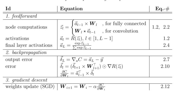
Table 2.1 Equations for training a simple CNN.

Id Equation Eq.-#

1. feedforward

node computations ~zl =

(

~al−1×Wl , for fully connected Wl? ~al−1 , for convolution

1.2, 2.2

activations ~al =R~(~zl),l ∈[1, L−1] 1.2

final layer activations ~aL = exp ~zL−1 P exp~zL−1 2.4 2. backpropagation output error ~δL=∇aC =~aL−~y 2.7 error ~δl = (~δl+1×Wl>+1) ∇R(~zl) 2.10 ∂C ∂Wl =~a > l−1×~δl 3. gradient descent weights update (SGD) Wi+1 =Wi−α_∂∂C_Wi 2.12

Table 2.1 describes all the equations required to train a neural network consisting of fully connected layers and convolutional layers.

2.2.4

Regularization

When a network is trained on a set of training data, it can perform worse with images that it has never seen before. This is called overfitting to training data. One of the most effective ways of disrupting a network’s tendency to overfit is to

prevent parameter co-adaptation with a technique called dropout. Dropout refers to deactivating random neurons for one forward pass during training, which prevents them from participating in backpropagation. This computationally inexpensive method causes the neurons of the network to learn to make more general ”observations” on the data, independent of the presence of particular neurons in the surrounding layers. [13]

Another very common method of input regularization is called data augmentation. Data augmentation means expanding the initial set of labelled images by adding slightly transformed duplicates. Some such transformations include flipping, rotating, shifting and blurring.

In supervised learning, data is not infinite as it cannot be generated. As such, the same input data may be shown to the network multiple times over the course of a single training session. Each set of iterations over which the network sees the whole input data set is called an epoch.

Dropout is generally effective in increasing the ability of a single neuron to produce more generally useful output. In practice, this results in better ability of the resultant model to generalize, improving accuracy on test set. Dropout has been found by Krizhevsky et al. to approximately double the time that it takes their model to converge [20]. The resultant models are still large, and it has been found that further reductions in size can be achieved by eliminating a large number of parameters in the resultant network.

While the inputs of a network are determined by the data, and the outputs by the use case, the structure and number of hidden units can be adjusted to get the best network performance. The number of hidden units non-trivially influences the network’s propensity for overfitting. A good practical solution is to choose a model with a high performance on a validation set. The validation set is a set of images chosen to be left out of the training set. [2, p. 256]

In this study, the best models are chosen based on validation set performance, and the reported accuracy is based on another set called the test set, which is also separated from the training data.

L2 regularization

Overfitting can be controlled by reducing model complexity. A good approach for doing this is to first choose a relatively high number of hidden units, then pressure weights towards 0, i.e. penalizing model complexity. This can be achieved by adding a regularization term to the error function~δ. [2, p. 256]

Two common techniques for penalizing model complexity are L1 _{regularization}

and L2 _{regularization. Results by Han et al. suggest that the L}1 _{regularization}

gives the best results after retraining. Both convolutional and fully connected layers can be pruned. By just pruning a network without retraining, they were able to achieve a 2× reduction in the number of connections. With retraining, the number of connections was reduced by 9×[11].

Bishop et al. describe the regularization term as

e

δ(W) =~δ(W) + λ 2W

>_{W, (2.13)}

where λ is the regularization coefficient that defines the resultant effective model complexity.

Bishop et al. write that regularizers that are not invariant to linear transformations favor some equivalent models over others, so they introduce a regularizer that is invariant to linear transformation [2, p. 258]:

λl

2

X

w∈Wl

w2_{. (2.14)}

Correctly choosing the regularization term λ forL2 _{pruning is important.}

Choos-ing a too largeλ results in a simple, underfit model, since more weights get squeezed to zero. Choosing a small lambda makes the model larger and more prone to overfit-ting. This can be seen as the accuracy on the validation set being larger than the accuracy on the test set.

In this thesis, L2 _{regularization is used in conjunction with masking of weights}

during training. This makes the fully connected layers have significantly fewer nonzero weights in total, effectively reducing model complexity.

2.3

Proposed optimizations

In this study, three strategies for reducing the model size of a pre-trained network were used: threshold pruning, pruning withL2 _{regularization, and separable convolutions.}

The effect on model size and performance was studied. Some parts of the network are more efficiently run on a graphics processor, and OpenCL was used to enable that.

2.3.1

Weights pruning

The aim of pruning weights is to reduce the total amount of values and computations required in a fully connected layer. Neural networks are often over-parameterized [7], which helps weights pruning be an effective technique in making the model smaller. Weights pruning during training has long been used as a technique for regulariza-tion. In an early work by Le Cun et al. [22], they identified and dropped the least significant weights in a network to improve its ability to generalize in classification,

and to speed up training of the model. There has been a lot of recent research interest in reducing the model size by reducing the number of weights and connections. In 2015, Han et al. [11] reduced the number of parameters of AlexNet by a factor of 9× and of VGG-16 by a factor of 13× without loss in accuracy. They did this by removing connections below a threshold and retraining the network afterwards using

L2 _{regularization. This process could be repeated multiple times to achieve final}

accuracy and to minimize network complexity. This is also one of the approaches used in this thesis.

2.3.2

Sparse models

A recent study by Zhu et al. [34] found that sparsified large models consistently outperform respective dense models of equal memory footprint across many domains. A particularly relevant class of optimizable models is that of the MobileNets [14], where Zhu et al. were able to reduce the number of parameters by 50 % with a 1.1 %-point reduction in top-1 accuracy and no reduction in top-5 accuracy.

Pruned weights matrices can be stored as sparse matrices. In this study, com-pressed row storage (CRS) format is used to represent a sparse matrix. In the format, the original matrix is encoded as non-zero (nnz) values and nnz indices along a selected axis. These compressed matrices require 2a+n+ 1 values where a is the number of nnz elements andn is either the number of rows or the number of columns [10].

The format was probably first introduced in 1967 by Tinney and Walker [31] and first fully described by Bulu¸c et al. [3]. Note that in this work, the CRS/CCS (compressed column storage) format is used instead of the more general compressed sparse blocks (CSB) format that Bulu¸c et al. describe. The CRS format allows efficient computation of theAx or the AT_{x matrix-vector product where A is an m}

byn sparse matrix and xis a dense vector of length n. Either the Ax or theAT_x

computation can be made efficient, depending on if CRS or CCS is used for matrix storage.

2.3.3

Separable convolutions

Using weights pruning to compress models has been found to be effective for the weights of the fully connected layers but less so for the kernels of the convolutional layers. Li et al. achieved inference cost reduction of 38 % on the CIFAR102 _training

set with negligible loss in accuracy by pruning out entire filters. He et al. were able to reach 2 × speed-up on state of the art networks ResNet and Xception but

2

with a significant 1.4 % and 1.0 % reduction in accuracy respectively [12]. Kernel factorization is an alternative to pruning entire channels or filters.

Jaderberg et al. [17] showed that the learned full rank kernels can be approximated by two rank-1 kernels. For a scene text character recognition application implemented in Caffe (CPU), this nets a 4.5× speedup with a 1 %-point reduction in accuracy or a 2.5× speedup with no degradation in accuracy. Their scheme 2 optimization seems to give best results in practice, as described by Jaderberg et al. [17]. They also showed that at least in their test case, the separable convolutions optimization scheme produces slightly better results than FFT based CNN optimizations. Scheme 2 means approximating a single convolutional kernel with two rank-1 basis kernels, one vertical and one horizontal:

S? ~x=~v ?(~h ? ~x).

Here, ? is again used to denote cross-correlation. Rank-1 kernels ~v and~h are defined as

~vk∈Rd×1×C :k ∈[1..K], (2.15)

where K is a hand-picked dimension for an intermediate feature map, and

~hf ∈R1×d×K :f ∈[1..F], (2.16)

where F is the number of feature maps in the original unoptimized network.

This optimization scheme reduces the complexity of computation fromO(k2_{CF H}0_W0₎

toO(F KH0W0), where W0 and H0 are the dimensions of the output feature map. In deep learning terms, each unoptimized convolutional layer is replaced by two decomposed rank-1 layers. The separated vertical convolution produces an intermediate feature map that is then convolved with a set of horizontal kernels. These kernels are learned by minimizing data reconstruction error, i.e. by aiming to reconstruct the outputs of the convolutional layers [17]. Jaderberg et al. minimize data reconstruction error asL2 _error:

min {~_{hk,f},{~vc,k}} n X i=1 F X f=1 ||Wf ? ~al−1(~xi)− C X c=1 K X k=1 ~hk,f? ~vc,k? ~al−1(~xi)||2. (2.17)

Equation 2.17 can be intuitively understood as minimizing the mean squared error (or L2 _{error) between the outputs of the unoptimized convolutional layer and}

the outputs of the optimized layers. This operation is done layer by layer and the kernels can be optimized as part of backpropagation. Jaderberg et al. note

that just replacing the original convolutional layers with the optimized ones for backpropagation results in model overfitting. Trying to combat the problem with approaches such as dropout make the model underfit instead [17]. Thus, the best approach to train the kernels is by data reconstruction as in Equation 2.17.

This optimization is effective if K(F +C)<< F Ck [17]. For the network under study, in the first layer F = 32, C = 3, k = 3, and K is selected as K = 7. Thus

K(F +C)< F Ck =⇒ 245<288. In the second layer: F = 32, C = 32, k= 3, and K is selected as K = 7. ThusK(F +C)<< F Ck =⇒ 448<<3072.

Depthwise separable convolutions

In this study, Jaderberg’s separable convolutions are used to optimize the con-volutional layers. However, other similar approaches have been developed. An optimization called the depthwise separable convolution was first introduced in 2014 by Sifre [29]. This means separating the convolution operation into two steps: depthwise and pointwise convolution. This strategy was used successfully by Howard et al. in 2017 to optimize convolutional neural networks for resource constrained platforms [14]. In their paper, they also introduced two simple hyperparameters that could be used to trade off between network latency and accuracy. Networks optimized with this strategy are called MobileNets, and they are available as part of the TensorFlow software library.

3 Implementation of optimizations

To compare the different optimizations described in Section 2.3, a convolutional neural network design by Huttunen et al. [15] was selected as a baseline implementation. The network is described in terms of dataflow programming, which facilitates easy altering of some aspects of the implementation.

Multiple versions of the different layers of the network were implemented and combined to get a view on how the optimizations stack up w.r.t. each other. In this chapter, an outline of the network to be optimized is first given, followed by descriptions of the implementations of these optimized layers and the final optimized networks formed of them.

3.1

Use case: a convolutional network for car type

recogni-tion

The network under study is a network for vehicle classification (VCN) by Huttunen et al. [15]. This is a 5-layer1 _{CNN with 1.88 million parameters, resulting in a}

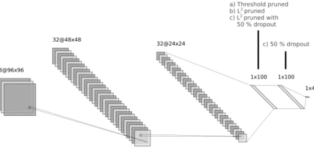
model size of 7.18 MB. It was trained using 6555 sample images collected originally in collaboration with Visy Oy2 _{[15]. An illustration of the general structure of the}

network is presented in Figure 3.1. The first two layers are convolutional layers with max pooling and ReLU as post-processing. The layers three and four are fully connected layers with ReLU post-processing. The last layer is fully connected, with softmax to process the values into action probabilities. There are 4 action probabilities, one for each type of vehicle: bus, car, truck, and van.

Figure 3.1 Illustration of the vehicle classifier network by Huttunen et al. (®2016 IEEE)

The structure and inference implementation of the network for a single image can be particularly understandably expressed in a Matlab-like pseudo code as in

1_{The number of adaptive layers of weights is used to count the number of layers in a network [2,}

p. 229].

2

Listing 1. Note that as an exception for this code sample, shapes are indexed in

Fortran-order3 as is done in Matlab code.

%% Non-trivial function explanations % read_jpg(file):

% reads a 3-channel jpg image from a `file` as 32-bit floats

% read_f32s(file):

% reads a series of 32-bit floats from a `file`

% get input and weights

input_image = reshape(read_jpg('image.jpg'), [96, 96, 3])

conv1_weights = reshape(read_f32s('w_conv1.bin'), [5, 5, 3, 32])

conv2_weights = reshape(read_f32s('w_conv2.bin'), [5, 5, 32, 32])

fc3_weights = reshape(read_f32s('w_fc3.bin'), [24*24*32, 100])

fc4_weights = reshape(read_f32s('w_fc4.bin'), [100, 100])

fc5_weights = reshape(read_f32s('w_fc5.bin'), [100, 4]) % layer 1 activations a1 = relu(convolve(input_image, conv1_weights)) a1_mxp = maxpool(a1) % layer 2 activations a2 = relu(convolve(a1_mxp, conv2_weights)) a2_mxp = maxpool(a2) % layer 3 activations

a2_mxp_reordered = reshape(a2_mxp, [24*24*32, 1]) a3 = relu(a2_mxp_reordered * fc3_weights)

% layer 4 activations

a4 = relu(a3 * fc4_weights) % layer 5 activations (softmax) z5 = a4*fc5_weights

a5 = exp(z5)/sum(exp(z5))

Listing 1 Matlab-like pseudo code for single-image inference.

The original network by Huttunen et al. was trained using backpropagation with

3

learning rate 0.001643. The reported accuracy of the network is based on the weights selected at 30,000 iterations, though the accuracy of the network seemed to converge already in 15,000 iterations in 20 minutes on Nvidia Tesla K40t GPU. The dropout technique was utilized between each layer to reduce the effect of overfitting. [15]

During measurements described in Chapter 4, it was found that the first fully connected layer of the network is highly redundant. Pruning the fully connected layer revealed that many parameters can be removed, as a similar network accuracy can still be achieved with only around 1 in 1000 of the weights retained in the network. This makes it interesting to test if simple threshold pruning would be an effective method in quickly and easily eliminating a high amount of least impactful weights. It is also interesting to see how pruning withL2 _{regularization affects the network.} L2 _{pruning was found effective by Han et al. in a very general case [11], and there}

is redundancy available in the network under testing. In the 2017 study, Zhu and Gupta also found that large-sparse networks like this tend to be more effective than theirsmall-dense counterparts [34].

3.2

Implementation of training

The network under optimization is trained like the original network [15] using TensorFlow API, with weights for separated convolution attained by minimizing data reconstruction error, i.e. Jaderberg’s approach. The network is then pruned with either of the two pruning strategies described next.

3.2.1

Pruning

Two different pruning strategies are used. In threshold pruning, some weights are periodically and permanently set to zero based on a threshold. These weights are masked out of the network for the remainder of training. Threshold T(to) is defined

as

T(t0) = min(Wl) +t0(max(Wl)−min(Wl)), (3.1)

where the threshold parameter t0 represents pruning sensitivity. Setting pruning

sensitivity to 0.0 would mean no pruning, and setting it to 1.0 would mean pruning everything, leaving the model empty. After pruning, the model is retrained until convergence.

In L2 _{pruning, the model is regularized, masked as in threshold pruning, and}

retrained. It was found via experimentation that early stopping each retraining at 10 epochs allows the model to fit to the training data. Regularization, masking and retraining is chosen to be applied in steps as follows:

2. repeat in 10 stages:

(a) eliminate parameters below halfway-through the current weight range:

T = 1₂(max(Wl) + min(Wl)),

(b) mask the zeroed weights out of the network,

(c) retrain or tune for 10 epochs with L2_{-regularization using regularization}

term λ.

After each tuning step, the model is accepted if its validation accuracy has degraded less than 1 %-point from accuracy of the baseline initial unpruned model on the validation data set. Note that the validation accuracy on the augmented data set may differ from the baseline accuracy reported previously by Huttunen et al. [15]. Tuned models are saved as long as the validation accuracy keeps increasing.

3.2.2

Assessment of model accuracy and overfitting

The images used for training the network are separated into three sets: training (90 %, 14108 images), validation (6 %, 898 images) and test set (4 %, 655 images).

The model is first fitted into the training set over a set amount of epochs. Next, the accuracy of the model on the validation set is assessed, and the accuracy on the test set is stored with the validation accuracy. The best validation accuracy is always kept, and the respective test accuracy is what is reported. Divergence of test accuracy from validation accuracy is also used to assess overfitting.

3.3

Inference optimizations

Every algorithm is run on a specific device. The structure and function of a com-putational device strongly affects how a layer transformation can be applied most efficiently. The modern computer processing unit works fastest when input values are read in the order they are used in the computation, organized into blocks of appropriate size. In terms of computer memory, an array that is organized like this without any extra space in between values is said to be contiguous.

A modern CPU is often capable of applying one operation to multiple contiguous elements, i.e. single instruction, multiple data (SIMD) of Flynn’s taxonomy [25]. Modern graphics processors (GPUs) use a similar model: single instruction, multiple threads (SIMT). Processors can often combine multiple mathematical operations together, eg. the multiply-accumulate (MAC) operation and fused multiply-add (FMA). To leverage these features, some vendors have created their own APIs and toolkits that can be used to optimize the program code for a particular device. However, in this thesis, only cross-platform optimization schemes are used: the LLVM compiler infrastructure and OpenCL.

Inference code and benchmarks were written in Rustand OpenCL.Rust is a

relatively new, open-source, systems programming language by Mozilla Foundation.

Rust is compiled with rustc of the LLVM compiler infrastructure. Part of the

inference code was written in OpenCL, that was then compiled by the driver on

each target device. OpenCL is a computing language by Khronos Group, Inc., used

for describing algorithms for GPUs and other highly parallelized processors.

The inference works in two steps: initialization and execution. During initializa-tion, the OpenCLdevices are selected and the OpenCL code is compiled by the

driver for the selected devices. Then the network graph is built into an OpenCL

command queue, and the weights are loaded into theOpenCL buffers.

After the timed execution starts, the input image buffer is loaded onto the GPU, and the OpenCL command queue is allowed to execute. After operations,

queue.wait() is called on the command queue to wait for the output buffers to flush and the operations to complete. An implementation for manually executing the inference graph across multiple devices is given in Listing 2.

In the inference implementation of Listing 2, input is mapped to the GPU buffer. This code is considered ”unsafe” in Rust, because it uses an underlying C-API to

control OpenCL, and the compiler cannot verify the memory safety of that code.

After mapping inputs, the OpenCL kernels for convolutions 1 and 2 are run. These

can be run on GPU or CPU based on instructions given per measurement. The buffer is then copied to the secondary device, which may be a GPU or a CPU. This is a no-op if the primary and secondary devices are the same. Next, the output buffers are copied onto the host memory for application of the final two fully connected layers. On the last line, softmax is applied to outputs, and the result is returned.

3.3.1

Sparse matrix multiplication

Training and pruning of weights was implemented using the TensorFlow API via Python. An optimized inference runtime4 was implemented in Rust. The main

component of the optimized inference runtime is the sparse matrix storage format. The sparse matrix storage format was first described by Tinney and Walker [31] and it is used as implemented in the community library Rustcrate sprs5.

In the sparse storage format, a matrix containing both zero and nonzero values (nnz) can be represented as three one-dimensional arrays. The arrays are as follows:

1. nnz values,

2. an accumulating counter of nnz values by row in original matrix, padded with a zero in the beginning,

4_{https://github.com/hegza/vcn-inference-rs}

let mut event_list = EventList::new(); // GPU ops are unsafe

unsafe {

map_to_buf(&input_buf, input_data).unwrap();

// Enqueue the kernel for the 1st layer (Convolution + ReLU) conv1_kernel.cmd().enq().unwrap();

// Enqueue the kernel for the 2nd layer (Convolution + ReLU) conv2_kernel.cmd().enq().unwrap();

// Copy GPU buffer to host conv2_out_buf

.copy(&dense3_in_buf, None, None) .enew(&mut event_list)

.enq() .unwrap();

// Enqueue the 3rd layer (fully connected)

dense3_kernel.cmd().ewait(&event_list).enq().unwrap(); }

// Wait for all on-device calculations to finish cl.cpu_queue.finish().unwrap();

// Read buffer into host memory

let dense3_out = &unsafe { read_buf(&dense3_out_buf).unwrap() }; // Run the 4th layer (fully connected)

let dense4_out = relu(dense4.compute(&dense3_out));

// Run and return the 5th layer (fully connected + softmax) softmax(dense5.compute(&dense4_out))

Listing 2 VCN inference code.

3. column indices of nnz values.

Consider a matrix with zeroes like

   0 1 0 7 3 0 0 0 0   .

/// computes matrix multiplication in_buf * wgts, /// when wgts is column-compressed

pub fn sprs_mtx_mul(

wgts: &sprs::CsMat<f32>, in_buf: &[f32],

out_buf: &mut [f32]) { let mat = wgts.view();

// creates an iterator over the columns of the matrix // and associated indices

for (col_idx, vec)

in mat.outer_iterator().enumerate() {

let mut acc = 0f32;

// creates an iterator over the rows of the matrix for (row_idx, &value) in vec.iter() {

acc += in_buf[row_idx] * value; }

out_buf[col_idx] = acc; }

}

Listing 3 Calculatingv×M inRustwithsprs.

// nonzero values

let nnz = [ 1, 7, 3 ];

// number of accumulated nonzeros by row let nnz_counter = [ 0, 1, 3, 3 ];

// column indices of nonzeros let col_idxs = [ 1, 0, 1 ];

This matrix is stored in the sprs library as CsMat. In practice, the transpose of the weights matrix needs to be computed instead of the original matrix. This is compensated for by using column compression instead of row compression. In a column compressed matrix, row indices are stored in the third array instead of column indices. This also changes nnz values to run from top-to-down then left-to-right. A

3.3.2

Separable convolutions

Weights for separable convolutions were trained using the approach by Jaderberg et al. by minimizing data reconstruction error in TensorFlow. Intuitively, this

means that the aim is to train the separated rank-1 kernels to produce feature maps that are as similar as possible to the feature maps produced by the original kernels.

Training is started by having the set of the original trained weights, and a set of untrained weights for the separable convolutions. The difference between the feature maps generated by each is then minimized using gradient descent, as shown in Equation 2.17 in Subsection 2.3.3.

These trained weights are then loaded in the Rust / OpenCL inference code

for benchmarking. OpenCL code for separable convolutions is provided at https: //github.com/hegza/vcn-inference-rs/blob/master/src/cl/sepconv.cl.

4 Measurements

Network performance was measured on multiple different representative platforms. Platform specifications are presented in Table 4.1.

Table 4.1 Platforms by given name.

Name CPU GPU Operating system

AMD desktop Phenom II X6 1090T Radeon HD 7800 Windows 10

Intel i7 Intel i7-2640M N/A Arch Linux

Mali ARM Cortex-A72×2/-A53×4 ARM Mali T860 Linux Firefly 4.4

Of the platforms presented in Table 4.1, AMD desktop is a typical desktop computer with a mid-tier GPU with 2 Gb of global memory and an OpenCL work

group size of 256. Intel i7 is an a typical mid-tier laptop and Mali is a representative embedded platform, used in single-board computers. SoCs of similar performance are used in contemporary smartphones, like the Samsung Exynos 5422 chip in Samsung Galaxy S5.

The structures of the trained networks are described in Table 4.2.

Table 4.2 Network structures by given name.

Name L1 L2 L3 L4 L5

VCN Conv Conv FC FC FC

VCN-sepconv SepConv SepConv FC FC FC

VCN-sparse Conv Conv Sparse FC FC

Conv is the baseline implementation of cross-correlation between weights and inputs. SepConv is the optimized separable convolution implementation. Fully connected layer (FC) is the baseline matrix multiplication implementation between weights and inputs, and Sparse is the pruned fully connected layer. Activations are rectifier linear unit (ReLU) or softmax.

4.1

Data collection

A set of weights was first trained to baseline accuracy (>97 %) in TensorFlow,

using a training set of 6555 images augmented to 14108 images by flipping and Gaussian blurring some of the images at random. The set of images was then separated to 12555 training images, 898 validation images, and 655 test images, which were used as-is forL2 _{pruning methods, but with changes for threshold pruning,}

as detailed in Subsection 4.1.1. The trained models were then pruned with three strategies. The first strategy used threshold pruning that clamps the values below the thresholdT of the range of the weight to be zero, and then eliminates them from