June 2018
NASA/CR–2018-219836
Multidisciplinary Design Optimization and
Cruise Mach Number
Study of Truss-Braced
Wing Aircraft
Rakesh K. Kapania, Mitchell Professor, Joseph A. Schetz, Fred D. Durham, Wrik Mallik, Molly C. Segee, and Rikin Gupta,
Virginia Polytechnic Institute and State University, Blacksburg, Virginia
NASA STI Program . . . in Profile
Since its founding, NASA has been dedicated to the advancement of aeronautics and space science. The NASA scientific and technical information (STI) program plays a key part in helping NASA maintain this important role.
The NASA STI program operates under the auspices of the Agency Chief Information Officer. It collects, organizes, provides for archiving, and disseminates NASA’s STI. The NASA STI program provides access to the NTRS Registered and its public interface, the NASA Technical Reports Server, thus providing one of the largest collections of aeronautical and space science STI in the world. Results are published in both non-NASA channels and by NASA in the NASA STI Report Series, which includes the following report types:
TECHNICAL PUBLICATION. Reports of completed research or a major significant phase of research that present the results of NASA
Programs and include extensive data or theoretical analysis. Includes compilations of significant scientific and technical data and information deemed to be of continuing reference value. NASA counter-part of peer-reviewed formal professional papers but has less stringent limitations on manuscript length and extent of graphic presentations.
TECHNICAL MEMORANDUM. Scientific and technical findings that are preliminary or of specialized interest, e.g., quick release reports, working
papers, and bibliographies that contain minimal annotation. Does not contain extensive analysis. CONTRACTOR REPORT. Scientific and
technical findings by NASA-sponsored contractors and grantees.
CONFERENCE PUBLICATION.
Collected papers from scientific and technical conferences, symposia, seminars, or other meetings sponsored or
co-sponsored by NASA.
SPECIAL PUBLICATION. Scientific,
technical, or historical information from NASA programs, projects, and missions, often
concerned with subjects having substantial public interest.
TECHNICAL TRANSLATION. English-language translations of foreign scientific and technical material pertinent to NASA’s mission.
Specialized services also include organizing and publishing research results, distributing specialized research announcements and feeds, providing information desk and personal search support, and enabling data exchange services. For more information about the NASA STI program, see the following:
Access the NASA STI program home page at http://www.sti.nasa.gov
E-mail your question to [email protected] Phone the NASA STI Information Desk at
757-864-9658 Write to:
NASA STI Information Desk Mail Stop 148
NASA Langley Research Center Hampton, VA 23681-2199
National Aeronautics and Space Administration
Langley Research Center Prepared for Langley Research Center Hampton, Virginia 23681-2199 under Contract NNL10AA05B
June 2018
NASA/CR–2018-219836
Multidisciplinary Design Optimization and
Cruise Mach Number Study of Truss-Braced
Wing Aircraft
Rakesh K. Kapania, Mitchell Professor, Joseph A. Schetz, Fred D. Durham, Wrik Mallik, Molly C. Segee, and Rikin Gupta,
Available from:
NASA STI Program / Mail Stop 148 NASA Langley Research Center
Hampton, VA 23681-2199 Fax: 757-864-6500
The use of trademarks or names of manufacturers in this report is for accurate reporting and does not constitute an official endorsement, either expressed or implied, of such products or manufacturers by the National Aeronautics and Space Administration.
1
SUGAR Phase III at Virginia Tech
Rakesh K. Kapania, Mitchell Professor, Department of Aerospace and Ocean Engineering Joseph A. Schetz, Holder of Fred D. Durham Chair, Department of Aerospace and Ocean Engineering
Wrik Mallik, Postdoctoral Research Associate, Department of Aerospace and Ocean Engineering Molly C. Segee, Graduate Research Assistant, Department of Aerospace and Ocean Engineering Rikin Gupta, Graduate Research Assistant, Department of Aerospace and Ocean Engineering Virginia Polytechnic Institute and State University, Blacksburg, VA, 24061
2
Contents
List of Figures ... 3 List of Tables ... 4 Acknowledgments... 5 Abstract ... 5 Nomenclature ... 6Multidisciplinary Design Optimization and Cruise Mach number Study of Truss-Braced Wing Aircraft ... 7
Introduction ... 7
Methodology ... 8
Design Constraints and Design Variables ... 9
SBW and TBW Design Configurations ... 10
VT MDO Assumptions ... 11
Comparison of VT MDO Methods and Boeing SUGAR II As-Drawn Design ... 11
Optimization Results ... 14
Optimization Results for Cruise Mach Number 0.70 ... 14
Optimization Results for Cruise Mach Number 0.80 ... 16
Transonic Aerodynamics Analysis for Multidisciplinary Design Optimization Applications ... 19
Methodology ... 22
Results and Discussion ... 24
Transonic Aeroelastic Analysis for Multidisciplinary Design Optimization Applications ... 32
Introduction ... 32
Methodology ... 34
Steady two-dimensional correction factors ... 34
State-space aeroelastic analysis of a wing ... 35
Reduced-order aerodynamic modeling ... 36
Results ... 37
Validation of the present approach for transonic flutter analysis ... 37
Validation of the ROM ... 40
Discussion ... 45
3
List
of
Figures
Figure 1. Pfenninger’s [3] vision of TBW ... 7
Figure 2. Typical Mission Profile of the aircraft studied ... 8
Figure 3. Flow of VT MDO calculations within ModelCenter TBW Framework ... 9
Figure 4. SBW Design Configuration Layout ... 10
Figure 5. TBW Design Configuration Layout ... 11
Figure 6. Fuel Weight v/s Take-off Weight at Mach= 0.70... 14
Figure 7. Fuel Weight v/s Flutter Margin at Mach= 0.70 ... 15
Figure 8. Minimum Fuel Weight configurations for TBW and SBW at Mach= 0.70 ... 15
Figure 9. Fuel Weight v/s Take-off Weight at Mach= 0.80... 17
Figure 10. Fuel Weight v/s Flutter Margin at Mach= 0.80 ... 17
Figure 11. Minimum Fuel Weight configurations for TBW at Mach= 0.80 ... 17
Figure 12. Empirical buffet boundary from Ref. 21 and 22 ... 22
Figure 13. Mesh for 10% thickness-to-chord ratio BACJ airfoil ... 23
Figure 14. Mesh independence check ... 24
Figure 15. Pressure coefficient results for 10% thickness-to-chord ratio BACJ airfoil at a lift coefficient of 0.335 and a freestream Mach number of 0.8 ... 25
Figure 16. BACJ airfoil wave drag coefficient vs lift coefficient for freestream Mach numbers from 0.7 to 0.95 ... 25
Figure 17. Surfaces fit to wave drag results at constant thickness-to-chord ratio ... 26
Figure 18. Center of pressure location vs lift coefficient for BACJ airfoil for freestream Mach numbers from 0.7 to 0.95 and comparison to empirical prediction ... 27
Figure 19. Surfaces fit to center of pressure location results at constant thickness-to-chord ratio28 Figure 20. BACJ airfoil lift coefficient vs. angle of attack for freestream Mach numbers from 0.7 to 0.95 ... 29
Figure 21. BACJ airfoil lift-curve slope vs lift coefficient and freestream Mach number for three thickness-to-chord ratios ... 30
Figure 22. Empirical buffet boundary for a BACJ airfoil for freestream Mach numbers from 0.7 to 0.95 ... 31
Figure 23. BACJ airfoil maximum allowable lift coefficient vs freestream Mach number for different thickness-to-chord ratios ... 32
Figure 24. Transonic flutter flowchart from Ref. [47] ... 35
Figure 25. Comparison of unsteady lift and moment responses between those obtained from indicial functions and unsteady RANS at k=0.202 [47] ... 38
Figure 26. Comparison of flutter boundary for 8% thick BACJ airfoil between unsteady RANS, indicial approach and linear Prandtl-Glauert (PG) [47] ... 39
Figure 27. Comparison of the flutter boundary predicted by the present method and NASTRAN DLM with the experimental results, for the WTM [47] ... 39
4 Figure 28. Nondimensional velocity-damping diagram for NACA 64A006 airfoil and wing strip
theory ... 41
Figure 29. Idealized cantilever wing ... 42
Figure 30. ZAERO g-method flutter results for an idealized cantilever at 8,000 ft. ... 42
Figure 31. Idealized cantilever wing: Mode 1, 1st out-of-plane bending mode ... 43
Figure 32. Idealized cantilever wing: Mode 2, 2nd out-of-plane bending mode ... 43
Figure 33. Idealized cantilever wing: Mode 5, 1st torsion mode ... 44
Figure 34. LB method flutter results for idealized cantilever at 8,000 ft. ... 44
Figure 35. Details of ROM eigenanalysis ... 45
List
of
Tables
Table 1. Design Load Cases ... 9Table 2. Design Metric for SUGAR II As-Drawn Configurations in Analysis Mode ... 13
Table 3. Design Metrics for VT SUGAR III (TBW and SBW) at M=0.7 ... 15
Table 4. Design Metrics for VT SUGAR III (TBW and SBW) at M=0.8 ... 18
Table 5. CPU time for each eigenvalue analysis ... 41
5
Acknowledgments
The research was funded by NASA under a SMAART contract to the Boeing Company. The authors thank Christopher Droney and Chester Nelson for many valuable technical discussions.
Abstract
The SUGAR Phase III was led by Dr. Rakesh K. Kapania and Dr. Joseph A. Schetz at the Multidisciplinary Analysis and Design Center for Advanced Vehicles, Department of Aerospace and Ocean Engineering, Virginia Tech, Blacksburg VA. The research was performed from December 2014 to December 2015. Three major areas were investigated:
Multidisciplinary Design Optimization (MDO) studies of truss braced wing (TBW) and strut braced wing (SBW) vehicles at cruise Mach numbers of 0.7 and 0.8 for a flight mission similar to current market single aisle configurations. The performance and the characteristics of the optimized vehicles were compared to the SUGAR Phase II TBW vehicle. These results were obtained without applying any of the extended transonic aerodynamic and aeroelastic tools that will be discussed later. It was found that the cruise Mach number has a large effect on the best “truss” configuration. At Mach 0.7, an SBW has a better fuel consumption and better take-off gross weight (TOGW). However, at Mach 0.8, the TBW is superior because the jury strut aids in satisfying the flutter constraint.
Two-dimensional, steady, transonic aerodynamic analysis of the Boeing Airfoil J (BACJ) airfoil was performed for a range of thickness ratios, Mach numbers and lift coefficients. Reynolds-averaged Navier-Stokes (RANS) equations were solved to obtain the lift-curve slope, wave drag coefficient, the location of the center of pressure and to predict the separation at the trailing edge, which may lead to buffeting. One of the goals was to develop a database of lift-curve slope and the location of center of pressure, which could be used in a transonic aeroelastic analysis. Another goal was to compare the wave drag coefficients to those predicted by Lock’s fourth-power law [3-6] and also to compare the transonic effects obtained from RANS simulations to those predicted by the Korn equations [10]. A third goal was to develop a buffet boundary, which can be integrated into the MDO framework to prevent the optimized designs from probable buffeting. A state-space transonic aeroelastic analysis tool was developed, which can incorporate the
nonlinear transonic effects in the unsteady aerodynamics but is yet computationally cheap when used within the VT MDO framework. The aeroelastic analysis uses Leishman-Beddoes (LB) [45-46] indicial functions, which generated a state-space representation of the aeroelastic system. The indicial functions allow the incorporation of data for steady lift-curve slope and location of the center of pressure. Thus, the steady transonic effects are included, and the unsteady aerodynamic responses are a linearization about the steady results. The aeroelastic approach discretizes the wing into numerous strips, which results
6 in a large eigenvalue problem as each strip has eight augmented aerodynamic states as per the LB theory. Thus, to reduce the computation expense, a reduced order model (ROM) was developed. The approach was validated using a few examples.
Nomenclature
c Chord
cd Two-dimensional drag coefficient
cdw Two-dimensional wave drag coefficient
cl Two-dimensional lift coefficient
cm Two-dimensional pitching moment coefficient about the quarter chord
CDW Three-dimensional wave drag coefficient
Cf Skin friction coefficient
CL Three-dimensional lift coefficient
Cm Three-dimensional pitching moment coefficient about the quarter chord
h Bending degree of freedom
Moment of inertia
L/D Lift-to-Drag ratio
M Local Mach number
m Mass per unit length
Q Generalized aerodynamic force
q Pitch rate
S Distance traveled in semichords, 2 U t/c
Sstrip Area of a wing strip
Sref Reference area based on wing planform
Static mass moment
t Time
t/c Thickness-to-chord ratio
U Local air velocity
V∞ Freestream velocity
xcp Center of pressure location
Angle of attack
κa Korn technology factor
Λ Wing leading edge sweep angle Frequency
Torsion degree of freedom
Wt. Weight
Mchordwise Chordwise Mach number Mstreamwise Streamwise Mach number
Mdrag divergence Streamwise drag divergence Mach number Mcrit Critical Mach number
7
Multidisciplinary
Design
Optimization
and
Cruise
Mach
number
Study
of
Truss
‐
Braced
Wing
Aircraft
Introduction
Limited oil resources and increasing fuel prices have led to intensive research of more efficient aircraft. One of the main factors affecting the fuel consumption of an aircraft is the amount of drag it produces. According to the study conducted by United States Department of Transportation (US DOT), in year 2015, the commercial aviation consumed 16.22 billion gallons of fuel with a cost of 46.27 billion dollars [1-2]. So, even a 1% reduction in fuel consumption would save millions of gallons of fuel annually. Many restrictions and constraints imposed on the structural aspects of a cantilever wing restrain it from further benefits. During the 1950s, Pfenninger [3] proposed the design of a truss-braced wing for transonic aircraft to achieve an increase in span and reduction in the thickness-to-chord ratio and wing sweep but with higher complexity as shown in Figure 1. Following Pfenninger’s ideas, the concept of SBW and TBW configurations for civilian transport aircraft has been extensively investigated using a multidisciplinary design optimization (MDO) approach [4-11]. These studies clearly establish the potential benefit of these configurations.
Figure 1. Pfenninger’s [3] vision of TBW.
The current study explores TBW configurations at Mach 0.7 and Mach 0.8, for current market single-aisle configurations aircraft mission with a payload of 30800 lbs. and a range of 3500NM. Different configurations have been considered: a truss-braced wing (TBW) configuration and the strut-braced wing (SBW) configuration. Figure 2 provides a schematic of the mission profile.
8
Figure 2. Typical Mission Profile of the aircraft studied.
Previous studies of SBW and TBW concepts at Virginia Tech have shown that both SBW and TBW configurations provide a significant reduction in fuel consumption for Boeing 777-200 ER and Boeing 737-800 NG types of missions[7-11]. So minimization of fuel consumption was the primary objective of this study. The TBW configurations were developed with the fuselage from the SUGAR II [12] public report with a DC-9 type T-Tail and the GE gfan+ engine [12]. The optimized TBW and SBW designs for all four configurations have been compared and analyzed.
Methodology
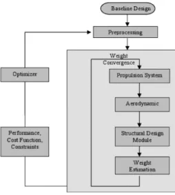
The MDO study was performed using the ModelCenter [13] interface, which serves as a link between the various analysis nodes and optimization nodes. The analyses are performed by in-house VT codes, which are linked to the ModelCenter interface via C++ or Python plug-ins known as Wrappers (see Figure 3). Details about the various wrappers and their purposes have been explained in detail in previous studies [4-11]. The aircraft is designed for 17 load cases, which represent various flight conditions as shown in Table 1. The first four load cases are the aircraft maneuver load cases. The fifth load case is a taxi bump load case that evaluates the wing-tip deflection for a 2-g landing associated with this transport mission [14, 15]. The remaining 12 load cases are used to calculate the gust loads as specified by Federal Aviation Regulations (FAR). As can be seen from Table 1, the loads are evaluated at conditions with different amounts of fuel weight. However, the present MDO framework does not account for the aeroelastic effects while computing the load distribution on the wing at various flight conditions. Thus, the load alleviation that may be provided by change in wing twist due to change in fuel weight or the aerodynamic loads is not accounted for. The MDO code assumes that the aerodynamic distribution would be the one that will lead to minimum induced drag and that the aircraft will have the jig shape that will lead to a twist distribution that would yield minimum induced drag.
9
Figure 3. Flow of VT MDO calculations within ModelCenter TBW Framework.
The entire process of optimization was carried out using a Genetic Algorithm (GA). The genetic algorithm used for this study is Darwin [16]. Detailed information about Darwin has been explained in previous publications [6, 9, 11 and 16].
Table 1. Design Load Cases.
.
Design Constraints and Design Variables
Design constraints have been imposed on the aircraft geometry and performance to ensure that the design satisfies the requirements of the flight mission. There are certain performance constraints placed on the initial cruise rate of climb, the second segment climb, the range of the design and
No. Alt [ft.] Mach N-Aero N-Inertia % Fuel % Cargo Title
1 36000 0.700 2.500 2.500 100.00 100.00 +2.5g,100%Fuel 2 36000 0.700 2.500 2.500 50.00 100.00 +2.5g,50%Fuel 3 36000 0.700 -1.00 -1.00 100.00 100.00 1g,100%Fuel 4 36000 0.700 -1.00 -1.00 50.00 100.00 1g,50%Fuel 5 0.0000 0.200 0.00 2.000 100.00 100.00 2g,Taxi_Bump 6 0.0000 0.200 - - 100.00 100.00 Gust,Approach,TOGW 7 0.0000 0.200 - - 10.00 100.00 Gust,Approach,Residual 8 0.0000 0.400 - - 100.00 100.00 Gust,0[ft.],TOGW 9 0.0000 0.400 - - 10.00 100.00 Gust,0[ft.],Empty 10 10000 0.500 - - 100.00 100.00 Gust,10000[ft.],TOGW 11 10000 0.500 - - 10.00 100.00 Gust,10000[ft.],Residual 12 20000 0.600 - - 100.00 100.00 Gust,20000[ft.],TOGW 13 20000 0.600 - - 10.00 100.00 Gust,20000[ft.],Residual 14 30000 0.700 - - 100.00 100.00 Gust,30000[ft.],TOGW 15 30000 0.700 - - 10.00 100.00 Gust,30000[ft.],Residual 16 40000 0.700 - - 100.00 100.00 Gust,40000[ft.],TOGW 17 40000 0.700 - - 10.00 100.00 Gust,40000[ft.],Residual
10 some limitations applied on the approach velocity and landing and takeoff distances based on FAA regulations.
Flutter margin was also added as one of the design constraints. The flutter analysis was conducted using the k-method with unsteady aerodynamics calculated using Theoderson’s theory. The flutter margin for braced wings (SBW or TBW) is always performed including the stress-stiffening effect. Thus, the stressed modal frequencies and the flutter speed are always functions of the load cases. However, such in-plane stresses are computed via linear static analysis. While a nonlinear static analysis would enable incorporation of the nonlinear geometric effects, it is not considered for the MDO studies owing to the computational expense associated with it. During the evaluation of the critical flutter margin, the flutter margins due to various load cases are computed and compared. The worst flutter margin is considered as the critical one to be applied as the constraint in the optimization study.
There are also some other constraints that impose limitations on the maximum wing-tip displacement during landing and a geometric constraint that rules out infeasible aircraft geometries. Further details about the various constraints are available in previous publications [5, 8, 11 and 17].
Design variables of the current TBW configuration contain the nongeometric and geometric design variables provided in previous studies [5, 8, 11 and 17]. The nongeometric design variables are average cruise altitude, the takeoff fuel weight, and the maximum required thrust. The geometric design variables constitute the wing planform and geometry of the truss members. The other geometric parameters remain constant throughout the process of optimization.
SBW and TBW Design Configurations
The VT MDO framework has the capability to perform design optimization for three types of configurations namely, Cantilever, SBW (Strut-Braced Wing) and TBW (Truss-Braced Wing) respectively. The SBW configuration has a strut attached to the high wing as shown in Figure 4 below.
Figure 4. SBW Design Configuration Layout.
The TBW configuration has an additional jury member as can be seen in Figure 5 below. The jury member provides additional support to the wing, thereby further reducing the bending stresses in the inner wing. It also reduces the effective length of individual truss members, thereby reducing
11 the possibility of strut or jury buckling during a -1g load case. However, it also generates additional interference drag.The MDO code includes all these effects and comes up with the most appropriate solution, a strut-braced or a truss-braced wing aircraft.
Figure 5. TBW Design Configuration Layout.
VT MDO Assumptions
Lift on the strut and jury is not considered, and no drag increment for landing gear pods is included.
0% drag reduction from riblets
Current Natural Laminar Flow (NLF) Technology factor and a Korn Factor = 0.887 gfan+ ducted fan engine with Specific Fuel Consumption (SFC) = 0.22 at Sea Level Static
(SLS) as mentioned in the SUGAR II Report and the DC-9 type T-Tail Latest VT structural model for better estimate of torsional stiffness
2015 Flutter Constraint [17] without the latest transonic aerodynamics added to the MDO
Comparison of VT MDO Methods and Boeing SUGAR II As‐Drawn Design
The VT MDO code can be used in two different modes:
1. Design Mode: In Design Mode, the MDO is carried out using Darwin (the genetic algorithm) optimizer or the gradient based optimizer.
2. Analysis Mode: In this mode, parameters like the guess-TOGW, fuel weight, thrust, etc., are provided as inputs. Converged TOGW, L/D ratio, the lift and the drag coefficients are obtained as output. No design optimization is performed.
In order to get a thorough understanding about the aerodynamics and the weight of the aircraft, the Boeing SUGAR II As-Drawn configuration was run in Analysis mode with different aerodynamics and the latest VT structural module (which gives a better estimate of torsional stiffness). Different technology factors as defined in the VT MDO, were used during the analysis mode calculations:
Body Riblets Turbulent Friction Factor: This factor multiplies the turbulent flat-plate friction coefficient, Cf, calculated for the bodies. It is used to simulate the use of riblets
12 Wave Drag Airfoil Technology Factor: The airfoil Korn factor influences the wave drag
calculation. The range is from 0.87 to 0.95 [10]. 0.87 represents the NACA 6-digit airfoil, while 0.95 represents a supercritical airfoil.
Natural Laminar Flow Technology Factor: In this case “nTransitionMode”=1. This is the technology factor for the chordwise transition Reynolds number for lifting surfaces.
Current technology based on current wings (0).
Aggressive laminar case based on F-14 NLF glove experiment (1).
If the value is between 0 and 1, an extrapolation is done. In any case, the chordwise location of the transition is limited by “dMaxLaminarFlowRatio”.
Several cases for the As-Drawn configuration were studied, and results for four cases are presented here to show the comparison of the VT SUGAR II As-Drawn configuration with the Boeing SUGAR II As-Drawn Configuration [12]. The Body Riblets Turbulent Friction Technology factor, Wave Drag Airfoil Technology factor and the Natural Laminar Flow (NLF) Technology factors were varied for these analysis mode calculations. The analysis mode calculations were made on the following assumptions:
Lift on the strut and the jury is not considered and no drag increment for landing gear pods were considered.
Gfan+ ducted fan engine with SFC = 0.22 @ SLS as mentioned in the Boeing SUGAR II Report and the DC-9 type T-Tail.
Latest VT structural model for better estimate of torsional stiffness
The flutter constraint was not considered during the Analysis Mode calculations
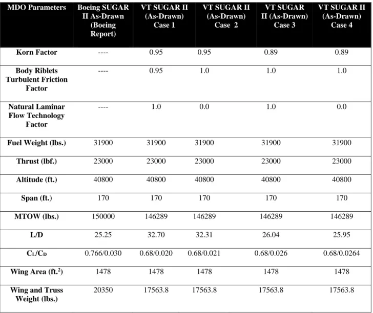
In the design metrics, MTOW, fuel weight, thrust, altitude, and span are the input parameters. After running the analysis mode, the MDO gives the output in terms of the converged MTOW, fuel weight, thrust, altitude, span and calculated L/D ratio, CL/CD, wing area and wing and truss system weight. Results are shown in Table 2.
Looking at the design metrics in Table 2, we mainly observe how a change in the Korn Factor affects the L/D ratio of the aircraft. Case 1 represents the design using highly aggressive aerodynamics with 5% reduction using body riblets turbulent friction technology along with aggressive NLF technology factor and a very high Korn factor of 0.95. This case has a 29% higher L/D ratio and 3.2% less TOGW than the Boeing result. This reduction in TOGW is mainly due to lower wing and truss weight for this configuration. Case 2 uses 0% reduction using the body riblets turbulent friction technology factor along with the current technology factor for NLF and the same Korn factor of 0.95. There is a very slight difference in terms of L/D ratio. Moreover, the TOGW and the wing and the truss weight system for this case also remains the same. For Case 3, we reduced the Korn factor to 0.89 with an aggressive NLF technology factor. This reduction in Korn factor further reduced the L/D ratio by 20.3% bringing it closer to the Boeing SUGAR II As-Drawn configuration results. Finally, for Case 4, we used the NLF based current aerodynamics technology factor with the Korn factor of 0.89. This change reduced the L/D ratio to 25.95 reducing
13 the difference between the Boeing SUGAR II As-Drawn and the VT SUGAR II As-Drawn configuration to 2.7%.
Table 2. Design Metric for SUGAR II As-Drawn Configurations in Analysis Mode.
MDO Parameters Boeing SUGAR
II As-Drawn (Boeing Report) VT SUGAR II (As-Drawn) Case 1 VT SUGAR II (As-Drawn) Case 2 VT SUGAR II (As-Drawn) Case 3 VT SUGAR II (As-Drawn) Case 4 Korn Factor ---- 0.95 0.95 0.89 0.89 Body Riblets Turbulent Friction Factor ---- 0.95 1.0 1.0 1.0 Natural Laminar Flow Technology Factor ---- 1.0 0.0 1.0 0.0 Fuel Weight (lbs.) 31900 31900 31900 31900 31900 Thrust (lbf.) 23000 23000 23000 23000 23000 Altitude (ft.) 40800 40800 40800 40800 40800 Span (ft.) 170 170 170 170 170 MTOW (lbs.) 150000 146289 146289 146289 146289 L/D 25.25 32.70 32.31 26.04 25.95 CL/CD 0.766/0.030 0.68/0.020 0.68/0.021 0.68/0.026 0.68/0.0264 Wing Area (ft.2) 1478 1478 1478 1478 1478
Wing and Truss Weight (lbs.)
20350 17563.8 17563.8 17563.8 17563.8
The calculations carried out in analysis mode helped us to understand how different technology factors affected the L/D ratio of the aircraft. It helped us achieve similar aerodynamics environments as Boeing in the VT MDO code. All the Case 4 inputs for the VT MDO during the analysis mode study shown above were applied in the design mode for carrying out the genetic based design optimizations for the SUGAR III designs.
14
Optimization Results
The basic objective of this study was to minimize the fuel weight for all four configurations and to analyze how other parameters change when we move from SBW to TBW. The best design will be the one showing the minimum fuel weight with the takeoff weight as low as possible. A graph of fuel weight v/s takeoff weight is plotted for each run, and the arrow on the figure points out the best design in terms of fuel weight. The color code represents the value of maximum thrust required by the aircraft. The design chosen was run further by seeding the genetic algorithm with best designs to make sure that the MDO converged. The images of the best designs were sketched using Visual Sketch Pad.
Optimization Results for Cruise Mach Number 0.70
The MDO results presented next are for the TBW and SBW at Mach 0.7. Figure 6 (a & b) presents the graphs of fuel weight v/s takeoff weight, and the arrows point out the best designs in terms of fuel weight. All the designs represented are feasible designs satisfying all the constraints including the flutter constraint. Figure 7 (a & b) show the graphs of fuel weight v/s flutter margin. From Figure 7 (a & b), the designs on the right hand side of the zero line satisfy all the constraints including the flutter constraint and the designs on the left violate the flutter constraint. For the TBW from Figure 7 (a), one can observe a cluster of designs that form almost a straight line. It also shows a very low fuel weight penalty to meet the flutter constraint. We also observe a similar trend for the SBW configuration. The aircraft configurations are shown in Figure 8. The numerical results in Table 3 indicate that the SBW configuration has a fuel weight of 16,030 lbs. and the TBW has 18,370 lbs. of fuel weight. The TOGW for the SBW is also ~10,000 lbs. less than the 132,219 lbs. of TOGW for the TBW. The wing and truss system weight of the SBW is ~7,000 lbs. less than the 22,291 lbs. of the TBW for the same mission profile.
15
Figure 7. Fuel Weight v/s Flutter Margin at Mach= 0.70.
Figure 8. Minimum Fuel Weight configurations for TBW and SBW at Mach= 0.70.
Table 3. Design Metrics for VT SUGAR III (TBW and SBW) at M=0.70.
S no Aspects VT SUGAR III
Min. Fuel Wt. (TBW) M = 0.7 VT SUGAR III Min. Fuel Wt. (SBW) M = 0.7 SUGAR II (As-Drawn) Boeing Report 1 MTOW (lbs.) 132219 122160 150000 2 Fuel Weight (lbs.) 18730 16030 31900 3 Thrust (lbf.) 13490 13470 23000 4 Altitude (ft.) 43776 48000 40800 5 Span (ft.) 181.1 217.7 170 6 Wing Area (ft.2) 1682 1821 1478 7 Aspect Ratio 19.49 26 19.56
16
8 Root Chord (ft.)/ t/c 11.67/0.084 12.47/0.0604 10.74
9 Tip Chord (ft.)/ t/c 4.35/0.077 3.96/0.0524 3.76
10 Strut Location/ Chord (ft.) 46.71/3.716 53.7/4.316 48.99/--
11 Wing and Truss Weight (lbs.)
22291 15216.3 20350
12 Wing Sweep (°) 4.4 4.39 12.52
13 L/D 36.2 41.2 25.25
14 Flutter Margin 1.048 % 6.954% -
We also observe that the aspect ratio of the SBW is 26 as compared to 19.49 for the TBW. The 33% increase in aspect ratio is one of the reasons why the SBW has a higher L/D of 41.2 than that of the TBW with 36.2. This leads to a reduction in induced drag, which further improves the efficiency of the aircraft by reducing the fuel weight by 14.4% to 16,030 lbs. The wing area of the SBW is slightly higher than that of the TBW, however, the t/c ratios are lower than that of the TBW leading to a lower wing and truss system weight for the SBW than the TBW. This reduction in wing and truss system weight helps in the reduction of the TOGW of the SBW compared to the TBW by approximately 7.7%. The relative benefits of the SBW compared to the TBW for this case is consistent with our earlier results for a 737-like mission.
Optimization Results for Cruise Mach Number 0.80
The MDO designs obtained from the optimization runs for the TBW and SBW at Mach 0.8 are shown in Figure 9(a & b). The figures provide a trade-study analogue between fuel weight and takeoff weight, and the arrows point out the best designs in terms of fuel weight. All of these designs are feasible designs satisfying all the constraints including the flutter constraint. In Figure 10 (a & b), a plot of fuel weight v/s the flutter margin is provided. The designs on the right hand side of the zero line in Figure 10 (a & b) satisfy all the constraints including the flutter constraint and the designs on the left violate the flutter constraint. For the TBW from Figure 10 (a), note a cluster of designs that form almost a straight line again showing a very low penalty to meet the flutter constraint. We observe a similar trend for the SBW configuration. These configurations are given in Figure 11. The results in Table 4 show that the SBW configuration has a fuel weight of 33,360 lbs., while the TBW has 26,760 lbs. of fuel weight. The TOGW of the SBW is also approximately 5000 lbs. more than the TOGW of the TBW with 151,204 lbs. However, the wing and truss system weight of the SBW is ~1800 lbs. less than the TBW of 26,880 lbs. for the same mission profile. This trend is opposite to the findings at Mach 0.7, where the SBW is preferred.
17
Figure 9. Fuel Weight v/s Take-off Weight at Mach= 0.80.
Figure 10. Fuel Weight v/s Flutter Margin at Mach= 0.80.
Figure 11. Minimum Fuel Weight configurations for TBW at Mach= 0.80.
One of the main reasons for the higher TOGW of the SBW in Table 4 is flutter. It leads to the SBW aircraft with reduced spans and lower aspect ratio wings. This in turn, affects the L/D, which
18 is 25% lower for the SBW than the TBW, leading to higher induced drag and higher fuel weight. The additional jury member in the TBW configuration plays a key role in reducing the flutter of the wing and the fuel weight, thus, providing additional support to the wing and permitting higher aspect ratio aircraft to achieve additional benefits.
The TOGW of the TBW at Mach 0.80 is 151,204 lbs. and the fuel weight is 26,760 lbs., 14.4% and 42.8% higher, respectively, as compared to a TBW optimized for Mach 0.7 cruise. The wing and the truss system weight is 26,880 lbs., which is 20% higher than that of the TBW at Mach 0.7. The reason for this behavior can be attributed to several factors. First, the span of the TBW at Mach 0.7 is 180 ft., and at Mach 0.8 it is 160 ft., approximately. This leads to higher induced drag which further reduces the L/D ratio of the aircraft leading to higher consumption of fuel for the same mission profile. Also at Mach 0.8, more pronounced transonic effects are observed. This is reflected as increased wave drag of the wing, further increasing the total drag coefficient. We can see this effect as the sweep almost doubles at Mach 0.8, delaying the drag divergence Mach number and the critical Mach number. The L/D ratio at Mach 0.8 is 24.5 compared to 36.2 at Mach 0.7. The L/D ratio reduces by 32.3% at Mach 0.8. The decrease in L/D ratio also leads to an increase in thrust by 61.2%. Second, the wing weight at Mach 0.8 is 20% higher mainly because of a 10.6% increase in surface area of the wing and the increase in strut chord by 62.1%. All these factors together contribute to a higher wing and truss weight system.
Table 4. Design Metrics for VT SUGAR III (TBW and SBW) at M=0.80.
S no Aspects VT SUGAR III
Min. Fuel Wt. (TBW) M = 0.8 VT SUGAR III Min. Fuel Wt. (SBW) M = 0.8 1 MTOW (lbs.) 151204 156543 2 Fuel Weight (lbs.) 26760 33360 3 Thrust (lbf.) 21770 23000 4 Altitude (ft.) 43900 42420 5 Span (ft.) 160.54 150.28 6 Wing Area (ft.2) 1861.05 1520.11 7 Aspect Ratio 13.84 14.87 8 Root Chord (ft.)/ t/c 13.49/0.038 12.41/0.065 9 Tip Chord (ft.)/ t/c 3.35/0.042 3.11/0/049
10 Strut Location/ Chord (ft.) 43.16/5.998 38.97/8.17 11 Wing and Truss Weight
(lbs.)
19
12 Wing Sweep (°) 9.8 9.89
13 L/D 24.5 18.11
14 Flutter Margin 2.12% 1.29%
Transonic
Aerodynamics
Analysis
for
Multidisciplinary
Design
Optimization
Applications
Multidisciplinary design optimization (MDO) methods require a large number of possible configurations to be analyzed while searching for an optimum. This often limits transonic aerodynamic calculations to computationally inexpensive, semi-empirical methods, which do not always accurately represent the physics. The center of pressure shift and the lift-curve slope change, both of which are required for accurate flutter calculations, are particularly difficult to predict using a semi-empirical approach. More accurate results can be found by specifying an airfoil shape and using computational fluid dynamics (CFD). However, this method is much more computationally expensive. To improve on this, Reynolds-averaged Navier-Stokes (RANS) CFD simulations are employed here on the BACJ airfoil to create a database of two-dimensional, aerodynamic coefficients and related values for a range of freestream Mach numbers, lift coefficients, and thickness-to-chord ratios likely to be used by the MDO code. The CFD calculations are performed in two dimensions to integrate the results with the strip theory formulation in the Virginia Tech MDO code and others. In addition, an empirical buffet boundary is applied to the results.
In the current VT MDO code, the 3D lift distribution is determined by a Trefftz plane analysis. The planform and the thickness-to-chord ratio variation and sweep are determined by the other analysis modules in the MDO iteration loop. The corresponding 2D values for each strip are found from the classical “strip theory” relations, which have proven especially useful for long, slender wings with low sweep.
Λ
20 Λ (2) Λ (3) cos (4)
Previously, these designs have been made without specifying an airfoil shape for the wings. To find the wave drag, the wing was divided into longitudinal strips with a known lift, thickness, and chord. The Korn equation was used to find the streamwise drag divergence Mach number for each strip based on the lift, the Mach number, the thickness-to-chord ratio, and an airfoil technology factor.
cos Λ cos Λ
| | 10 cos Λ
(5) Lock's fourth-power law was used to predict the critical Mach number for each strip, then to find the wave drag. See Refs 2-6 for more detail.
0.1 80 / (6) 20 if 0 if (7) More recently, the center of pressure, which is needed for flutter calculations, was simply assumed to vary linearly from 25% chord at a Mach number of 0.4 to 40% chord at a Mach number of 0.97 [20].
Obtaining better results for the drag, center of pressure shift, and lift-curve slope, variation in the transonic regime requires specifying an airfoil shape and using computational fluid dynamics (CFD). However, using CFD directly within the MDO would be prohibitively computationally expensive. Instead, CFD is used here to find the drag, wave drag, center of pressure, and lift-curve slope variation for a representative airfoil shape (BACJ) at numerous points over the range of
21 Mach numbers, lift coefficients, and thickness-to-chord ratios likely to be used by the MDO. The wave drag, center of pressure, and lift-curve slope variation at a given Mach number, lift coefficient, and thickness-to-chord ratio are found from these results by interpolation.
The wave component of the total drag was found from the pressure distribution. It was decided to use the database to predict wave drag, not total drag, because the CFD results do not take laminar-turbulent transition into account. As a result, the friction drag is still found with the method used previously in the MDO. An artificial neural network is used as a surrogate model for the wave drag. The input to this model is the two-dimensional lift coefficient, thickness-to-chord ratio, and freestream Mach number, and the output is the two-dimensional wave drag coefficient. Two layers of four nodes each are used for the neural network.
For small angles of attack, the center of pressure location can be found from the lift coefficient and the quarter chord moment coefficient with the following equation:
0.25 (8) Because the BACJ airfoil is cambered, the pitching moment coefficient is not zero when the lift is zero. This causes the center of pressure to have a discontinuity when the lift is zero and this discontinuity makes it difficult to fit a model directly to the center of pressure location. Instead, a
model is fit to the CFD results for the pitching moment coefficient, and Eq. +0.25 (8) is used to find the center of pressure location. An artificial neural network with two layers of
four nodes each is used as a surrogate model for the pitching moment coefficient. The input for this is the two-dimensional lift coefficient, thickness-to-chord ratio, and freestream Mach number. Two neural networks are used for the lift-curve slope model. The first is trained using the CFD lift coefficient results and uses angle of attack, thickness-to-chord ratio, and freestream Mach number as the input. It has one layer with ten nodes. By taking the derivative of this model with respect to angle of attack, the lift-curve slope can be found. However, this requires angle of attack as an input, which is not known by the MDO.
A second neural network is used to relate angle of attack to lift coefficient, thickness-to-chord ratio, and freestream Mach number. This model also has one layer with ten nodes. This model is used to find the angle of attack for a wing strip, then the first model is used to find the lift-curve slope.
An empirical buffet boundary was applied to the database results. There are a number of empirical relations that use the local Mach number before the shock and the shock location to predict the onset of buffet. Two of these relations, one from Lynch [21] and one from Fokker [22] are shown in Figure 12. There is not much difference between these relations. The Fokker boundary is used for buffet prediction in this report. This boundary only goes to 70% of the chord. When shocks
22 occur at greater than 70% of the chord it is unlikely that there will be enough interaction with the structure to allow the flow unsteadiness to be felt in the rest of the plane.
While the immediate motivation for this work is for application to our MDO studies of truss-braced wing transport aircraft, this database is equally useful for MDO studies of other conventional or unconventional configurations.
Figure 12. Empirical buffet boundary from Ref. 21 and 22.
Methodology
The CFD code used for this study is the Stanford University SU2 [23, 24] code, which is a steady, 2D RANS method. SU2 was used to find the lift, drag, wave drag, and pitching moment coefficients of the airfoil. The center of pressure and lift-curve slope at each point are found from these results. A Spalart-Allmaras turbulence model was used, and all cases were run at a Reynolds number, based on the mean aerodynamic chord, of 6×10⁶. This is done for Mach numbers from 0.7 to 0.95, lift coefficients from 0 to 0.8, and thickness-to-chord ratios of 6% to 10%. This is the range of values likely to be used by the MDO. A linear interpolation is used in the MDO to find aerodynamic coefficients and related values at a given Mach number, lift coefficient, and thickness-to-chord ratio using these results.
A BACJ airfoil shape was selected as representative of modern supercritical airfoils for transport aircraft. This airfoil has a thickness-to-chord ratio of 10.1%. Two other similar airfoils with thickness-to-chord ratios of 8% and 6% were created. The thickness perpendicular to the chord was scaled by moving the upper and lower surface points toward the midpoint between the two surfaces.
23 A separate mesh was made for each thickness-to-chord ratio. Each mesh has three regions. The first region is a structured, 1600×35 region near the airfoil surface to resolve the boundary layer. The cell spacing at the airfoil surface is 2.9×10⁻⁶, which results in y+ values near 1. The second region is a finer unstructured region to resolve the shocks. This region is circular with a radius of 1.5 chord lengths, is centered on the trailing edge, and contains 6×10⁴ cells. The rest of the mesh consists of a coarser, unstructured region containing 9×10³ cells. The cell counts given here are approximate. The exact number of cells varies between the three meshes used. The front of these meshes has a radius of 20 chord lengths, and the meshes extended 20 chord lengths behind the airfoil. See Figure 13.
Figure 13. Mesh for 10% thickness-to-chord ratio BACJ airfoil.
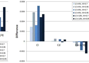
All three meshes used were found to be fine enough for mesh independent results. This was checked by comparing the results to results obtained from a mesh with approximately 4 times as many cells. This was done at the highest lift coefficient run for both the highest and lowest Mach number run for each thickness-to-chord ratio, for a total of six cases. The difference between the results for the two meshes is shown in Figure 14a, and the percent difference in the results is shown in Figure 14b.
24
Figure 14. Mesh independence check.
Results and Discussion
Figure 15 shows a comparison of results for inviscid, Euler equations and viscous, RANS equations. The case shown is for a lift coefficient of 0.335, a freestream Mach number of 0.8, and a thickness-to-chord ratio of 10%. The inviscid results have a considerably stronger and further aft shock than the viscous results. The inviscid results also have a shock on the lower surface which does not appear in the viscous results. As a result, the inviscid results predict a quarter-chord pitching moment coefficient that is much higher than the pitching moment coefficient predicted by the viscous results. This causes the center of pressure to move from 86% of the chord for the inviscid results to 70% of the chord for the viscous results. Because of the significant difference between the results for the two methods, viscous RANS equations were used to generate the database for the MDO.
The wave drag coefficient as a function of the lift coefficient for the airfoil is shown in Figure 16. It can be seen that the wave drag tends to increase with lift, Mach number, and thickness-to-chord ratio, as would be expected. However, for the 6% thickness-to-chord ratio and a lift coefficient of 0.8, the wave drag is higher for a Mach number of 0.7 than for a Mach number of 0.8. This may be due to the small leading-edge radius of the 6% thickness-to-chord ratio airfoil. The flow accelerates at the leading-edge, then begins to decelerate until near the center of the airfoil. Because the shock is further aft for a freestream Mach number of 0.8 than it is for a Mach number of 0.7, the shock is weaker.
25
Figure 15. Pressure coefficient results for 10% thickness-to-chord ratio BACJ airfoil at a lift coefficient of 0.335 and a freestream Mach number of 0.80.
Figure 16. BACJ airfoil wave drag coefficient vs lift coefficient for freestream Mach numbers from 0.70 to 0.95.
(a) Euler (b) RANS
(a) thickness-to-chord ratio of 6% (b) thickness-to-chord ratio of 8%
26 The neural network results for wave drag are shown in Figure 17 a-c. The CFD wave drag results are shown with red spheres. The root mean squared (rms) error between the neural network model and the CFD results is 0.0021.
Figure 17. Surfaces fit to wave drag results at constant thickness-to-chord ratio.
The center of pressure results are shown in Figure 18. Only the cases with positive lift are shown. Because the BACJ airfoil is cambered, the pitching moment is not zero when the lift is zero and this causes the center of pressure to go to infinity as the lift goes to zero. As a result, the location of the center of pressure is very dependent on lift. The center of pressure location also changes with Mach number. The center of pressure moves aft as the Mach number is increased until a Mach number of 0.9. After a Mach number of 0.9, the center of pressure begins to move forward as the Mach number is increased further. Figure 18d shows the center of pressure location predictions from the previous, simple empirical method used. This empirical method assumed that the center of pressure moved linearly from 25% of the chord at a Mach number of 0.4 to 40% of the chord at
(a) thickness-to-chord ratio of 6% (b) thickness-to-chord ratio of 8%
27 a Mach number of 0.95. It can be seen that this does not agree with the actual behavior, especially the strong dependence of the center of pressure location on the lift coefficient.
Figure 18. Center of pressure location vs lift coefficient for BACJ airfoil for freestream Mach numbers from 0.7 to 0.95 and comparison to empirical prediction.
The surrogate model for the center of pressure location is shown in Figure 19. The original points from the CFD results are shown with green spheres. The root-mean-squared error is 0.2972, which is somewhat high. However, if only points with lift coefficients greater than 0.05 are considered, the rms error is reduced to 0.0278. If the minimum lift coefficient is increased to 0.2, the rms error is reduced further to 0.0087. The majority of the error between the CFD results and the model is at points with very low lift coefficients, where the center of pressure location changes rapidly. At higher lift coefficients, this model has good agreement with the CFD results.
(a) Thickness-to-chord ratio of 6% (b) Thickness-to-chord ratio of 8%
28
Figure 19. Surfaces fit to center of pressure location results at constant thickness-to-chord ratio.
The lift coefficient for the BACJ airfoil vs. angle of attack is shown in Figure 20. The lift-curve slope is almost constant at a freestream Mach number of 0.7 for all the cases. As the freestream Mach number is increased, the presence of shocks and flow separation cause the slope to vary with lift. When the freestream Mach number is increased to 0.95, the upper surface shock is near the trailing edge. The shock does not move as the lift is varied, and the region of separated flow after the shock is small. As a result, the lift slope is essentially constant with angle of attack for cases where the freestream Mach number is 0.95.
(a) thickness-to-chord ratio of 6% (b) thickness-to-chord ratio of 8%
29
Figure 20. BACJ airfoil lift coefficient vs. angle of attack for freestream Mach numbers from 0.70 to 0.95.
The surrogate model for the curve slope is shown in Figure 21. This is compared to the lift-curve slope found directly from the CFD results for lift using second-order finite-difference equations, shown with green spheres. The rms error between the finite-difference results and the surrogate model is 1.3362. However, this is reduced by more than half, to 0.5793, when only points with lift coefficients between 0 and 0.8 are considered.
(a) Thickness-to-chord ratio of 6% (b) thickness-to-chord ratio of 8%
30
Figure 21. BACJ airfoil lift-curve slope vs lift coefficient and freestream Mach number for three thickness-to-chord ratios.
Figure 22 shows the two-dimensional lift coefficient at which buffet occurs as a function of freestream Mach number. Because we are not concerned with buffet at Mach numbers greater than the cruise Mach number, this relation does not go past a freestream Mach number of 0.8. To determine this limit, several cases were run at freestream Mach numbers at or below the cruise Mach number. An empirical relation from Fokker [22] is shown in Figure 12, which relates the local Mach number before a shock and the shock location to buffet was used to determine whether or not a case would buffet and how close that case was to the buffet limit. When a case was found that was at or just below this buffet limit, it was added to Figure 22.
Designs should not exhibit buffeting when the lift coefficient is increased to 1.3 times the cruise lift coefficient. Assuming that the lift distribution remains constant, this limits the lift coefficient at each strip to 0.77 times the lift coefficient at which buffet occurs. The VT MDO normally does not allow the two-dimensional lift coefficient at any location to be greater than 0.8. This means
(a) thickness-to-chord ratio of 6% (b) thickness-to-chord ratio of 8%
31 that the buffet limit is only a concern when it limits the lift coefficient to less than 1.04, 1.3 times 0.8.
When the shock location is greater than 70% of the chord, it is unlikely that there will be enough interaction with the structure to allow the flow unsteadiness to be felt in the rest of the plane.
Figure 22. Empirical buffet boundary for a BACJ airfoil for freestream Mach numbers from 0.70 to 0.95.
A neural network with one layer of three nodes was fit to the results in Figure 22 to relate the maximum allowable lift coefficient to the thickness-to-chord ratio and the freestream Mach number. A straight line is used to relate the thickness-to-chord ratio to the freestream Mach number at which the shock location is greater than 70% of the chord. The surrogate model for the maximum allowable two-dimensional lift coefficient before the buffet constraint is violated is shown in Figure 23. Note that neither axis starts at 0.
(a) thickness-to-chord ratio of 6% (b) thickness-to-chord ratio of 8%
32
Figure 23. BACJ airfoil maximum allowable lift coefficient vs freestream Mach number for different thickness-to-chord ratios.
Transonic
Aeroelastic
Analysis
for
Multidisciplinary
Design
Optimization
Applications
Introduction
All the flutter analysis performed for the TBW designs in the past assumed that the flow around the aircraft is incompressible or subsonic compressible flow. While these assumptions made the flutter analysis simple, they become inaccurate as the Mach number of the flow reaches 0.8 or above. In reality, this is where most commercial aircraft operate. Thus, a more accurate representation of the transonic flow is required to perform a better flutter analysis. The major shortcoming of the steady, subsonic, compressible, small-disturbance potential flow theory is that it is linear in nature and it provides incorrect predictions of the lift-curve slope and the location of center of pressure [25] about which a linearized unsteady aeroelastic analysis is to be performed. Secondly, it also cannot capture discontinuous physical phenomena like the appearance of shock waves [26, 27]. Thus, the aeroelastic analysis may lead to inaccurate results. To solve this problem, extensive computational fluid dynamic (CFD) simulations have been run at Virginia Tech to solve the Reynolds-Averaged Navier-Stokes (RANS) equations using the software SU2 [23-24]. The details are provided in the previous section.
Amongst the various approaches generally used for transonic flow such as the transonic small disturbance potential equations [28-31], the full potential equations [32], the Euler equations [33, 34] and the Navier-Stokes equations [35, 36], RANS equations are the most appropriate for the present work. Raj and Singer [37] have compared steady transonic predictions of the Euler and RANS solutions with experimental results for a Mach number envelope and an airfoil similar to the one studied here. They have shown that the shocks experienced by the flow would be far too
33 strong to neglect viscous effects like shock-boundary layer induced separation and the possibility of buffet. Euler or any other inviscid method cannot capture such viscous effects. Thus, RANS, supported by appropriate turbulence models, can capture the physical phenomena without going for a direct numerical simulation of the Navier-Stokes. Bendiksen provides a review of the various methods used for transonic aerodynamic analysis [27].
The unsteady aeroelastic analysis is a different problem altogether, and it is introduced as follows. It is known that the unsteady aerodynamic response of an airfoil under harmonic motion has two parts to it. One is an instantaneous response, which dies down exponentially over time. This response is due to the inertia of a body in a fluid domain when its motion is initiated. The other part is due to the circulatory response caused by the vortices shed by the body as it is disturbed. This motion develops with time and asymptotically reaches its steady-state value as the shed vortices reach infinity. These two effects must always be accounted for in an unsteady aerodynamic response evaluation. Theodorsen [38] developed a combination of Hankel functions to demonstrate the amplitude and the phase lag of the circulatory response to a small disturbance in incompressible flow for a step-change between two steady-state conditions. Such responses, termed as “indicial functions”, have the advantage that once they are known, the total response to an arbitrary time history of forcing can be developed using the superposition theory in the form of Duhamel's integral. The resulting lift and moment are a superposition of these two types of responses.
To obtain the counterparts of such functions in compressible flow, Mazelsky [39] and Mazelsky and Drischler [40] developed some responses but only at Mach numbers of 0.5, 0.6 and 0.7. Beddoes, appropriately scaled the circulatory indicial functions so that they can be developed as a generalized function of Mach number [41], and in his later work [42] developed a method to properly quantify the noncirculatory response by accurately predicting the time constants of the exponential functions representing this phenomenon. For his later work, he used the notion that an airfoil would start off as a piston with some normal downwash into a gas at rest [43]. Thus, at the initiation of the motion, the airfoil response, comprised of both the circulatory and noncirculatory components, would behave analogous to a piston, and this behavior is independent of the Mach number. Thus, he equated the rate of change of his total aerodynamic response at the initiation of the motion to the ones that Lomax [44] obtained for steady supersonic flow. This approach is used to obtain the time constants of the noncirculatory response. Leishman [45] developed an indicial response for pitching moment that includes the contribution of the pitch rate induced camber effects. This is important because the aerodynamic response of an airfoil would be similar for the angle of attack and plunge rates as both of them induce a constant downwash along the airfoil. However, the pitch rate leads to a linearly varying downwash. The present analysis uses an extended version of the Leishman-Beddoes (LB) indicial function where it is assumed that the lift acts at the center of pressure instead of the aerodynamic center. The behavior of the aerodynamic center in the transonic regime is complex and rather odd. Finally, a state-space formulation for the
34 linear system is generated similar to Leishman and Nguyen [46] to develop a linear stability analysis to determine the onset of flutter.
The state-space formulation with the LB model is a 2-D aerodynamic theory that is suited for an airfoil. However, we are interested in the development of low-order transonic flutter analysis tools for high aspect-ratio wings, which can be employed for conceptual aircraft design studies in an MDO environment. For this the LB indicial functions are first modified to include the corrections from steady 2D RANS simulations, and then applied to the individual strips of a high aspect-ratio wing discretized into numerous strips [47]. For the structure, a 3-D, 6 degrees of freedom finite element model (FEM) of the structure is developed, and a set of linear 1st-order ordinary differential equations (ODEs) is developed for the system with a large number of aerodynamic and structural states. These are then reduced to a much smaller number of states by modal transformation for the structure and reduced-order modeling (ROM) of the unsteady aerodynamics as explained later.
There are two parts to the development of the low-order transonic flutter analysis tool. One is the strip-theory based transonic flutter analysis with the modified LB indicial functions. This has been already discussed in Ref. [47]. Only key validation results from that study are presented here, and certain limitations of the approach are discussed. The other part is the ROM presented here. The development of this ROM has already been extensively discussed in Ref [48]. Benchmarking of the ROM is presented here. Finally, the computational efficiency of the reduced order approach is also discussed.
Methodology
Steady two‐dimensional correction factors
As presented earlier, a steady CFD response surface was prepared based on the two-dimensional RANS simulations. The response surface was developed offline by training neural networks to input data sets oflift coefficients, Mach numbers, and thickness ratios, and output data sets of lift-curve slopes and pitching moment-lift-curve slopes at the corresponding values of the inputs. The response surface can be subsequently used during online flutter analysis where the thickness ratio of the section, the Mach number and the lift coefficients can be provided as inputs, and the lift-curve slopes and pitching moment-lift-curve slopes to be used in the flutter analysis can be quickly obtained. A schematic illustrating the application of the steady CFD-based neural network-based response surface for online flutter analysis inside an MDO framework, is provided in Figure 24 [47]. An extensive discussion of the application of the response surface for online flutter analysis is also presented in Ref. [47].
35
Figure 24 Transonic flutter flowchart from Ref. [47].
State‐space aeroelastic analysis of a wing
Any linear system can be written in state-space form as:
9.1 9.2 where represents the states of the system, represents the inputs and represents the output. The matrices , , and have their usual definitions. The indicial functions provided in Ref. [45] by Leishman has been expressed in state-space form by Leishman and Nguyen [46]. A modified version of the indicial functions and the corresponding aerodynamic state-space system is provided in Ref. [47], which is valid for any location of pitch axis/elastic axis, and the pitching moment-curve slope is introduced directly into the indicial functions. The state-state aerodynamic formulation can be coupled with the equations of motion of an elastic structure to obtain the state-space aeroelastic formulation. Derivation of the aeroelastic state-state-space formulation for an elastic airfoil is provided in Ref. [47]. The finite element structural formulation of the wing can then be employed to assemble the airfoil aeroelastic system along the span of the wing, which has already been discretized along the span into several aerodynamic strips/structural elements. Detailed discussion of the treatment of the wing sweep, and the transformation of two-dimensional forces in the airfoil’s local coordinate system to the three-dimensional global coordinate system of the wing, is provided in Ref. [47]. The aeroelastic system of the wing can be represented in the state-space form as:
10
where I represents the identity matrix. , and represent the structural stiffness, structural damping and structural mass matrices in the global coordinate system, respectively. and represent the aerodynamic stiffness and aerodynamic damping in the global coordinate system, respectively. Matrices , and are related to the aerodynamic lag states and defined in
36 Ref. [47]. represent the states of the elastic system and . A detailed derivation is also provided in [47].
For the 3-D finite element structural model, there are 6 degrees of freedom at each node. The aerodynamic model has 8 augmented states per element or per strip. Thus, for n nodes and m elements, the eigenvalue problem becomes of the order 12 8 . To reduce the number of structural states as well as to develop diagonalized mass and stiffness matrices, a modal analysis is performed, and the first p modes of the structure obtained from an eigenanalysis of the free structural system are used. To reduce the number of aerodynamic states, a model reduction of the aerodynamic system is performed using a balanced model realization technique while matching the DC gains. This is discussed in the next section.
Reduced‐order aerodynamic modeling
The aerodynamic modeling is performed via strip theory with the LB model applied for each strip. Thus, there are 8 aerodynamic states for each strip, and there are 8 m aerodynamic states for the whole system having m elements. To reduce the size of the aerodynamic system and thereby reduce the size of the eigenvalue problem, reduced order aerodynamic modeling is implemented.
Several methods of reduced-order modeling (ROM) for unsteady flows are available. One of the earlier ones was by Hall [49] who performed an eigenanalysis of his zero-input, unsteady aerodynamic system obtained from the vortex lattice method. The eigenanalysis was able to diagonalize the zero-input aerodynamic matrix and also reduce the number of states required to represent the system. However, a quasistatic correction was required so that the contribution of the high frequency modes could be incorporated into the steady-state behavior of the system. Thus, the steady-state behavior included the contribution of all the modes, and the unsteady phase lag was characterized by the first few low-frequency modes. Romanowski [50] used a different method to perform the ROM where he used the time domain proper orthogonal decomposition (POD) technique, also known as Karhunen-Loeve expansions, to create a reduced-order aeroelastic model of a two-dimensional isolated airfoil, including compressible aerodynamics. Hall et al. [51] used the POD technique of an ensemble of small-disturbance, frequency-domain solutions to determine basis vectors for constructing the ROM. Other researchers have used the balanced realization technique to perform the aerodynamic model reduction via internally balanced modes [52, 53].
Here, a method is employed that adopts the balanced realization technique but in principle is similar to the eigenanalysis-static correction method presented by Hall. First, a balanced realization of the state-space system is performed to evaluate the grammians. Based on these grammians, the first few high frequency modes or fast modes of the system are selected. Subsequently, the model reduction is performed based on the selected fast modes. However, while doing so, the DC gains of the slow or low frequency modes are matched by performing a correction to the fast modes thereby ensuring that the steady-state behavior of the actual system is retained. The number of fast modes to be used for model reduction is problem dependent and is usually a
37 significant fraction of all the states of the full model. This is a feature of the asymmetric aerodynamic system, where the modes are not well separated unlike their structural counterpart. The algorithm for the matched DC gains method for continuous-time models is as shown below. Let the state-space system be defined by equations (9.1)-(9.2). The state vector is partitioned into
, to be kept, and , to be eliminated. Thus,
11 12 Next, the derivative of is set to zero, and the resulting equation is solved for . The ROM is given by
13.1
13.2 where a subscript of denotes that the aerodynamic matrices are reduced via balanced residualization. Note that the model-reduction method employed here is known as the method of matched DC gains or balanced residualization by the ‘controls’ community. Furthermore, the state-space system of first-order equations presented in equation (11) is for the unsteady aerodynamic system only. It is a state-space representation of the indicial functions, which are obtained by time-linearizing the actual unsteady system about steady-state responses. The model reduction thus aims to reduce the number of lag states required to represent the unsteady aerodynamics. If a reduced aerodynamic system is desired, equations (13.1) and (13.2) will substitute equations (9.1) and (9.2), respectively, in the derivation of the state-space aeroelastic formulations. The modified aeroelastic system with reduced aerodynamic matrices can be represented as,
14
Results
Validation of the present approach for transonic flutter analysis
Three cases discussed in Ref. [47] are presented here. First is the benchmarking of the RANS-corrected modified indicial functions, where the lift and pitching moment predicted via the present approach due to harmonic pitching is compared to the time-accurate RANS results obtained from
38 SU2. Second is the comparison of the flutter boundary predicted by the present approach for an 8% thick BACJ airfoil against time-accurate predictions from the SU2 RANS. Third is the comparison of the flutter boundary predicted by the present strip-theory-based approach for a TBW wind-tunnel-scaled model (WTM) against experimental results.
CaseI:Unsteadyresponseofan8%thickBACJairfoiltoharmonicpitching
An 8% thick BACJ airfoil was subjected to harmonic pitching at a Mach number of 0.8 and at a reduced frequency 0.202. The unsteady lift coefficient and pitching moment coefficient at the quarter-chord, obtained via the indicial method, is compared to unsteady RANS in Figure 25. Further details for this case are provide in Ref. [47]. The small differences between the indicial response and RANS are due to the unsteady shock dynamics that cannot be captured in the time-linearized indicial responses. This is more evident for the moment response as shock dynamics are known to affect the location of shock, thereby affecting the pitching moment at the quarter-chord.
Figure 25 Comparison of unsteady lift and moment responses between those obtained from indicial functions and unsteady RANS at k=0.202 [47].
CaseII:Flutterboundaryofan8%thickBACJairfoil
The flutter boundary predicted by unsteady RANS for the same 8% thick BACJ airfoil, is compared with its coun