Predicting individual stock returns using optimized
neural networks
Master’s Thesis
Jukka Song
Aalto University School of Business
Master of Science in Finance
Spring 2019
www.aalto.fi Abstract of master’s thesis
Author Jukka Song
Title of thesis Predicting individual stock returns using optimized neural networks Degree Master of Science
Degree programme Finance Thesis advisor(s) Matthijs Lof
Year of approval 2019 Number of pages 57 Language English Abstract
I investigate individual monthly U.S. stock return predictability through a comparative study on neural networks and ordinary least squares benchmarks, using a predictor set of 102 lagged firm characteristics and the market return from 1980 to 2018. I find monthly out-of-sample (OOS) R2 of 0.80% for the best neural network, confirming similar findings of marginal predictability from existing literature applying machine learning to empirical finance. OOS R2 increases to 7.12% for the best neural network, when considering average market return predictability using market return predictions constructed bottom-up from equal-weighting individual stock predictions. I also find significant monthly four-factor alphas of 1.55% and annualized Sharpe ratios of 2.62 on long-short top-bottom decile portfolios sorted on predicted returns – not taking into account trading costs. Investigating variable importances within neural networks reveals that networks using Rectifier as their activation function focus on momentum and liquidity variables, similar to existing findings, but networks using Maxout focus on firm fundamentals and risk measures instead – a new observation for the anomalies literature. Lastly, my findings confirm that return anomalies are stronger in small stocks, and prediction performance is generally stronger during market turbulence.
www.aalto.fi Maisterintutkinnon tutkielman tiivistelmä
Tekijä Jukka Song
Työn nimi Predicting individual stock returns using optimized neural networks Tutkinto Kauppatieteiden maisteri
Koulutusohjelma Rahoitus Työn ohjaaja(t) Matthijs Lof
Hyväksymisvuosi 2019 Sivumäärä 57 Kieli Englanti
Tiivistelmä
Tutkin Yhdysvaltalaisten yksittäisten osakkeiden kuukausittaisten tuottojen ennustettavuutta vertaillen neuroverkkoja pienimmän neliösumman menetelmään, käyttäen 102 yritysmuuttujan ja yhden markkinatuoton datasettiä vuosilta 1980-2018. Parhaan neuroverkon testiotannan R2 on 0.80%, varmistaen samankaltaiset löydökset ennustettavuuden tasosta
tutkimuksissa, jotka soveltavat neuroverkkoja empiiriseen rahoitustieteeseen. Testiotannan R2
nousee 7.12%:iin parhaan neuroverkon tapauksessa, kun on kyseessä keskimääräisen markkinatuoton ennustettavuus käyttäen markkinatuoton ennustuksia, jotka ovat laskettu yksittäisten osake-ennustusten keskiarvoista. Osake-ennustusten perusteella järjestetty portfolio, joka ostaa korkeinta ja myy alinta desiiliä, tuottaa 1.55% merkittäviä kuukausittaisia neljän tekijän alfaa ja 2.62 Sharpen lukua vuositasolla – huomioimatta kaupankäyntikustannuksia. Tutkittaessa ennustajien tärkeyttä neuroverkoissa huomataan, että verkot, jotka käyttävät Rectifier-aktivointifunktiota keskittyvät momentum ja likviditeetti muuttujiin, kun taas verkot, jotka käyttävät Maxout-aktivointifunktiota keskittyvät yritysten perustekijöihin ja riskin mittareihin, tuoden uuden löydöksen anomalioiden kirjallisuuteen. Löydökseni vahvistaa, että tuottoanomaliat esiintyvät vahvempina pienissä osakkeissa, ja ennustettavuus on yleisesti parempaa markkinoiden ollessa turbulentteja.
Contents
1. Introduction ... 5
2. Literature review ... 7
Predictability of stock returns ... 7
Proliferation of anomaly factors and the curse of dimensionality ... 8
Econometric methods to deal with model uncertainty and parameter instability ... 9
Machine learning methods suitable for high dimensionality, model uncertainty and parameter instability ... 9
3. Data ... 11
4. Methodology ... 12
Constructing training, validation and testing data sets ... 12
Over-arching function and methods ... 13
Benchmark ordinary least squares linear regression ... 15
Neural networks anatomy ... 15
Neural network hyperparameters ... 17
Hyperparameter tuning through random grid search ... 20
Controlling for randomness in model training and results through repetition ... 21
Measuring statistical prediction performance using out-of-sample R2, return correlation and directional accuracy ... 22
Measuring economic value of predictions: Bottom-up equity premium predictions and excess returns from machine learning portfolios ... 22
Measuring relative predictor variable importance ... 23
5. Analysis and results ... 23
Hyperparameter grid search results ... 23
Main results: Out-of-sample R2 compared to linear benchmarks ... 25
Standard deviations of out-of-sample R2 and correlation between in-sample and out-of-sample performance ... 27
Rolling past 12-month out-of-sample R2 over time ... 29
Correlation between predicted and realized returns and directional accuracy ... 31
Market premium perspective: Index return prediction accuracy ... 32
Neural network long-short portfolio results ... 36
Variable importance ... 40
6. Conclusion ... 45
7. References ... 48
1.
Introduction
The asset pricing literature has found significant cross-sectional stock return predictability (Avramov and Chordia (2006), Rapach and Zhou (2013), Jordan, Vivian and Wohar (2014), and Dangl and Halling (2012)). In parallel, hundreds of anomaly variables that produce excess risk-adjusted returns and correlate with firms’ subsequent stock returns have been discovered (Green, Hand, and Zhang (2013) and Hou, Xue, and Zhang (2017)). As traditional linear regression methods deal poorly with high-dimensional problems and model uncertainty, machine learning models that excel in such environments have been applied to enhance stock return predictability and gain new insights into which factors really provide independent information on stock returns (e.g. Gu, Kelly, and Xiu (2018)). My paper is largely motivated by the proliferation of anomaly variables discovered in the asset pricing literature, and the economic possibilities of understanding that information to predict stock returns with modern machine learning models.
In this paper, I study the predictability of individual stock returns based on a large set of fundamental predictor characteristics using neural networks. I use a set of 102 firm characteristics as Green et al. (2017) and the market return in a panel data to predict one-month-ahead U.S. returns for the sample period 1980 to 2018. My main focus is comparing various rigorously optimized neural network models to the baseline OLS regression predictions.
The paper contributes to the empirical asset pricing literature in three ways. First, I analyze the degree of stock return predictability for individual stocks, comparing machine learning to traditional methods. I evaluate predictability through statistical measures and economic profitability. From the statistical perspective, I find one of three chosen neural networks to consistently outperform OLS benchmarks across the measures with an average out-of-sample R2 of 0.80%, average correlation between predicted and realized returns of 9.66%, and average directional accuracy of 52.96%. Across the three statistical measures, neural networks outperform in correlation and directional accuracy, but the results are more mixed for out-of-sample R2. From the economic perspective, I construct stock portfolios sorted on predicted returns and evaluate the profitability of a long-short strategy on the top and bottom deciles. In terms of monthly returns and annualized Sharpe ratio, neural networks greatly outperform OLS benchmarks, with neural network portfolios returning as much as 1.51% on average per month, with a Sharpe ratio of 2.62, not accounting for trading costs. I also evaluate aggregate market return predictability by comparing the predicted and realized equal-weighted
average returns of market portfolios constructed from individual stock returns. I find that the results mirror those of individual stock predictions, where a few neural networks outperform in R2, and generally outperform in directional accuracy. Notably, the monthly out-of-sample R2 at a portfolio level increases to an average of 7.12% for the best neural network. Upon further analysis, most of the predictability stems from the lagged market return predictor and its nonlinear interactions with firm predictors. Models trained without the market return predictor generally fail to achieve positive out-of-sample R2. Additionally, upon analyzing result differences in 500 largest and smallest stocks, I find that all predictability measures confirm that predictability is stronger in small stock than big stocks (e.g. Green et al (2017)). I also analyze the time series of rolling out-of-sample R2 and cumulative returns of the neural network portfolios, which reveal that prediction performance is generally better during times of market turbulence, aligning with results of Dangl and Halling (2012).
Second, I identify predictor variables that contribute the most to return prediction in neural networks, contributing to the return anomalies literature where hundreds of factors have been found as statistically significant predictors of cross-sectional returns. Since neural networks learn the relation between predictors and predictions without a priori information from the researcher and allow for nonlinear complex relations, it may identify predictive power eluding conventional linear methods. I follow the Gedeon (1997) method of calculating relative variable importance based on predictor weights in the neural network and find two different results from two different neural networks: one confirms earlier findings of Gu et al. (2018) and Messmer (2017), where momentum (e.g. 1-month or 6-month momentum) and liquidity (e.g. return volatility or zero trading days) variables are most important, the other finds new evidence of the importance of firm fundamentals (e.g. cash or volatility of cash flow) and risk-based measures (e.g. beta or idiosyncratic volatility).
Third, I provide a rigorous neural network comparison, by conducting extensive random grid searches for optimal model topologies and controlling for inherent randomness of neural networks by repeating the training of each optimized network 100 times and reporting summary statistics. I find that there are significant differences in neural network performance in the noisy data environment of stock returns. Neural networks using the popular Rectifier as their activation function produced highly varied results when measured by out-of-sample R2, with standard deviations 0.42% compared to 0.12% of the next best neural network. Rectifiers also became unstable the most often during random grid search, where the majority of deeper Rectifier networks failed in training. The other two neural networks using so called Maxout
and Tanh activation functions performed more stable, generating results in a denser spread. Additionally, based on relative variable importance per neural network, Rectifier and Maxout models prioritize very different data to extract predictive information. Rectifiers use the momentum and liquidity, while Maxouts use firm fundamentals and risk measures. Thus, this paper provides researchers looking to apply neural networks to empirical finance with detailed insights on model optimization choices and resulting performance.
2.
Literature review
In the asset pricing literature, results for stock return predictability are mixed. Stock return predictability has been examined both through cross-sectional regressions that seek to model differences in expected returns across stocks on firm-level characteristics, and through time-series regressions on aggregate market returns on macroeconomic variables. There is an enormous literature (see for example Rapach and Zhou’s (2013) overview paper) documenting how various variables have predictive power of aggregate stock returns, such as the popular dividend-price ratio (Fama and French (1988)). However, the evidence for such predictability is predominantly in-sample. Goyal and Welch (2008) show in their influential paper for numerous economic variables in the literature that out-of-sample equity premium forecasts fail to consistently outperform the simple historical average benchmark forecasts in terms of mean square forecast error (MSFE).
Predictability of stock returns
Stock returns inherently contain a large unpredictable component, so that even the best forecasting models can explain only a small part of returns. In addition, market efficiency requires that when successful forecasting models or factors are discovered, they will also be adopted by others, which leads to the eventual disappearance of such predictability. On this point, McLean and Pontiff (2016) document a 58% decrease in post-publication returns based on a study of 97 variables and their out-of-sample post-publication return predictability. The maximum level of predictability in terms of monthly R2 is 8%, according to a loose analysis
by Rapach and Zhou (2013) of the typical predictive regression model. In practice, forecasting results for stock market aggregate returns are generally in the 1% neighborhood for in-sample tests, and lower out-of-sample: Fama and French (1988) report monthly R2 statistics of 1% or
less for predictive regression models based on dividend-price ratios, Zhou (2010) reports 1% or less for individual predictive regressions based on 10 popular economic variables, and Jordan et al. (2014) report over 2% out-of-sample for several European countries based on a combination of fundamental, macroeconomic and technical variables. These papers calculate R2 statistics comparing predicted returns to the historical average prediction. In comparison, a study by Gu et al. (2018) using machine learning algorithms to predict individual stock returns use a R2 statistic that compares predicted returns to a zero-return prediction, because the historical average comparison underperforms the zero-return prediction when considering individual stocks. Their study yields monthly R2 values of less than 1% at best. However, the literature agrees on that even small improvements in prediction accuracy can result in significant economic benefits (Campbell and Thompson (2008), Rapach and Zhou (2013)).
Proliferation of anomaly factors and the curse of dimensionality
The proliferation in the number of published anomaly variables that appear significant in explaining cross-sectional stock returns has led to the questioning of the validity of traditional methods in evaluating whether new characteristics really provide independent information about average returns, as asserted by Cochrane’s (2011) presidential address. Since the establishing of the CAPM of Sharpe (1964) and Lintner (1965), discoveries have been published on significant factors such as the size (Banz (1981)), value (Rosenberg, Reid, and Landstein (1985), Fama and French (1992)), and momentum (Jegadeesh and Titman (1993)) that have become mainstays in the widely used Fama and French (1993) three-factor and Carhart (1997) four-factor models. More recently in the past decades, the discovery of new anomaly variables has accelerated, resulting in hundreds of anomaly factors being published, as documented by Green, Hand, and Zhang (2013), where they analyze 333 return predictive signals, or Hou, Xue, and Zhang (2017), who conduct a replication study on 447 anomaly variables. However, these aforementioned critical studies are unified in their conclusion that most of the analyzed predictive signals do not appear significant, or their scale is much lower than originally published. Thus, there is serious evidence of p-hacking and data snooping in empirical finance (Chordia, Goyal, and Saretto (2018)).
To tame the factor zoo, many econometric methods have been applied to deal with the curse of dimensionality. For example, Giglio and Xiu (2016) and Kelly et al. (2017) use dimension reduction methods to test and estimate factor pricing models. Kozak et al. (2017)
construct a stochastic discount factor that summarizes the joint explanatory power of many cross-sectional stock return predictors. Freyberger et al. (2017) use the adaptive group LASSO to select characteristics to approximate a nonlinear function for expected returns. Feng et al. (2017) propose a model-selection method to systematically evaluate the contribution to asset pricing of any new factor. Sun (2018) uses a newly developed machine learning tool to regularize a large set of factors, grouping highly correlated factors while shrinking off the useless ones simultaneously. Though these attempts have shown promise and a reduction in the number of significant factors, there appears to be no consensus. This has led to Kozak et al. (2017) conclusion that the quest to summarize the cross-section of stock returns with sparse characteristics-based factor models to be ultimately futile, as there is not enough redundancy among the many return predictors.
Econometric methods to deal with model uncertainty and parameter instability
In addition to addressing high dimensionality, more recent strategies have improved forecasts by addressing model uncertainty and parameter instability concerns that traditional linear regression models ignore. Model uncertainty recognizes that a forecaster does not know the optimal model specification or the corresponding parameter values. Parameter instability recognizes that the model and its parameters may change over time. Rapach and Zhou (2013) describe four strands of forecasting strategies that deliver statistically significant out-of-sample gains: economically motivated model restrictions (Campbell and Thompson (2008)), forecast combination (Rapach et al. (2010)), diffusion indices (Neely et al. (2014)), and regime shifts (Dangl and Halling (2012)). Additionally, parameter instability has been investigated with time-varying coefficients, where Dangl and Halling (2012) find that models with time-varying coefficients dominate models with constant coefficients. They also find that stock return predictions are closely linked to business cycles, where stronger accuracy is achieved during recessions.
Machine learning methods suitable for high dimensionality, model uncertainty and parameter instability
Considering the discussed issues of high dimensionality, model uncertainty, and parameter instability, machine learning techniques provide attractive options. As described by Gu et al.
(2018), first, the task in asset pricing, of trying to understand the cross-section of asset returns or the aggregate market risk premium, is fundamentally about prediction, and machine learning methods are largely specialized for prediction tasks. Second, with its wide range of methods from linear models to regression trees and neural networks, machine learning is explicitly designed to deal with model uncertainty and complex nonlinear functions. Third, in the problem of high dimensionality due to hundreds of predictor variables, machine learning algorithms are well-capable of reducing dimensions and condensing redundant variation among highly correlated predictors.
The best performing machine learning models for stock return prediction have generally been neural networks and regression trees (Gu et al. (2018), Messmer (2017), Cao et al. (2005)), and improving on them, ensemble methods that pool and combine predictions from several different machine learning models (Tsai et al. (2011)).
Gu et al. (2018) conduct a comparative analysis on the performance of various machine learning algorithms in individual stock return prediction. Included are linear regression, generalized linear models with penalization, dimension reduction via principal components regression and partial least squares, regression trees (including boosted trees and random forests), and neural networks. Their analysis includes a large set of individual stocks over 60 years with a set of roughly 100 predictive variables. They find that allowing for nonlinearities substantially improves predictions, where trees and neural nets improve return predictions from a benchmark monthly stock-level R2 of 0.16% to R2’s between 0.27% and 0.39%. The benchmark is a panel regression of individual stock returns onto the lagged size, book-to-market, and momentum variables. When they run the analysis for bottom-up portfolio-level return forecasts of the S&P 500 index from stock-level forecasts, the monthly R2 for trees and neural networks is 1.39% and 1.80%, compared to the benchmark of -0.11%. The portfolio level prediction averages out more of the stock-level noise while boosting signal strength.
Messmer (2017) trains deep feedforward neural networks on a set of 68 firm characteristics to predict the U.S. cross-section of stock returns, finding that neural network long-short portfolios can generate attractive risk-adjusted returns compared to a linear benchmark. Cao et al. (2005) find the same result with Chinese stocks, where neural network models outperformed linear models. Tsai et al. (2011) use classifier ensemble methods to predict whether quarterly stock returns are positive or negative and find that classifier ensembles outperform single neural network models, and that the return on investment is better for all tested machine learning models than the buy and hold strategy. For the reasons, further
analysis on neural networks and their performance in stock return prediction is valuable and interesting. The goal of this paper is to provide a more rigorous examination of neural networks and analyze the prediction performance of optimized networks and infer information on which predictors are the most important.
3.
Data
I follow Green et al.’s (2017) influential paper in using the dataset from their website1 with 102
firm characteristics and monthly individual stock returns from the time period 1980 to 2018, totaling 38 years, with an average of around 4000 stocks per month. I also add one-month lagged market return as a predictor. The firm data is entirely calculable from CRSP, Compustat, or I/B/E/S data, and begins in 1980 due to most characteristics becoming robustly available only then. Details of the characteristics including sources, definitions, and percentage missing of each characteristic is provided in Table A1 in the appendix.
Green et al. (2017) begin the data creation with all firms with common stock on the NYSE, AMEX, or NASDAQ that have a month-end market value on CRSP and a nonmissing value for common equity in their annual financial statements. Data is integrated across Compustat, I/B/E/S, and CRSP and characteristics are computed and aligned in calendar time. For each month t’s return they calculate characteristics as they were at the end of month t-1. Also, annual accounting data is assumed to be available at the end of month t-1 if the firm’s fiscal year ended at least six months before the end of month t-1, and quarterly accounting data to be available if the fiscal quarter ended at least four months before the end of month t-1. Green et al. (2017) also include delisting returns in the monthly stock returns taken from CRSP, delete 20 observations that have a monthly return less than -100%, and set blank values of analyst following (nanalyst) to zero. The dependent variable is monthly returns in excess of the risk-free rate (XRET). Excess return is calculated as a stock’s monthly return minus the risk-free rate. The market return variable is based on the Wilshire 5000 Total Market Full Cap Index and the risk-free rate is the “3-Month Treasury Bill: Secondary Market Rate”. Both are retrieved from the economic research data base at the Federal Reserve Bank at St. Louis.
1 Dataset retrieved using the SAS code on their website:
4.
Methodology
The methodology applied in this paper consists of five steps. First, I split the entire data set into training, validation, and testing data. Second, I find the optimal neural network topologies used in further analysis through random grid searches. Third, I train three optimized neural networks 100 times each to produce 300 neural networks models to control for randomness among different iterations of the model, and compute three linear OLS benchmarks to compare against. Fourth, I generate predictions using the 300 neural networks and 3 OLS benchmarks and analyze average neural network prediction performance statistically and economically. Fifth, I analyze relative variable importance to infer which predictors are most impactful to the predictions.
Constructing training, validation and testing data sets
I split the data set into three subsets: training, validation, and testing sets. The training data set is used for training the model, where the model calculates the optimal parameter coefficients for the predictor variables. The validation data set is used during training (both in random grid search and training the optimized models) to enable “early stopping” regularization reducing overfit. The testing data is a true out-of-sample test of the tuned models, using data that has not been used for model training or validation.
Before creating the dataset splits, the characteristics are first winsorized at the 1st and 99th percentiles of their monthly distributions. Then, I split the data into a training set with 75% of all data (1980-2006) and testing set with 25% of all data (2007-2018). I shuffle the order of the training data set, as shuffling training data is considered best practice for neural networks to make learning more robust and less susceptible to time-specific outliers (Brownlee (2016)). Shuffling the training data breaks up the temporal order and enables the model to better learn information from the entire panel. I standardize the training dataset to zero mean and unit variance and store the standardization parameters (mean and standard deviation) for each characteristic. The reason to standardize the variables is both to deal with missing values, and to make neural network model training faster and reduce the chances of getting stuck in local optima (Sarle (2002)). Then, the testing set is scaled according to the stored parameters of the 75% training set. Scaling the testing dataset according to stored standardization parameters from the training set is done to avoid introducing future information of variable distributions
into the testing dataset. After standardizing and scaling the data, I set all missing values to the post-standardized mean of zero as Green et al. (2017).
Lastly, I create the validation dataset with 25% of all data by splitting a portion off from the training set. The validation dataset is thus also in a randomized order. Choosing a shuffled validation dataset instead of a time-period specific set (e.g. training using data from 1980 to 1997, then validation from 1998 to 2006) attempts to strike a reasonable compromise between trying to avoid a “lucky split” and being a representative out-of-sample test. A “lucky split” would mean, for example, that data in 1998 to 2006 could be unrepresentative of the general data, which would push the models to overfit to that period and result in poor true out-of-sample prediction performance later. The randomized validation dataset contains data from different time periods, so is more representative of general data, but is less “out-of-sample”, sacrificing some its representativeness as an out-of-sample test. However, none of the validation data is used during training, so it is still data the model has not seen. Also, since the feedforward networks I train do not explicitly learn temporal information from the order of the rows and the data is already in panel form, the order of data is less significant. I consider the potentially better k-folds cross-validation method but decide not to use it due to high computational cost and H2O not supporting cross-validation if recursive model refitting is done (which I do during the true out-of-sample testing).
The result is a shuffled and standardized training dataset with 75% of all data – from which I split a 50% training set and 25% validation set for hyperparameter tuning – and a temporally ordered and scaled testing dataset with 25% of all data.
Over-arching function and methods
We follow Gu et al.’s (2018) description of the over-arching functional form of the models utilizing panel data. In constructing predictive models for stock returns based on lagged information, the primary objective of the models is to minimize the mean squared forecast error (MSFE). Some regularization is imposed on the models through variations of the MSFE objective, in order to avoid overfitting and to improve out-of-sample predictive performance.
In its most general form, an asset’s excess returns can be described as:
𝑟𝑖,𝑡+1 = 𝐸𝑡(𝑟𝑖,𝑡+1) + 𝜀𝑖,𝑡+1
where
Stocks are indexed as 𝑖 = 1, … , 𝑁𝑡 and months as 𝑡 = 1, … , 𝑇. The predictive models construct a representation of 𝐸𝑡(𝑟𝑖,𝑡+1) as a function of predictor variables that minimizes the out-of-sample MSFE between the predicted return and realized return 𝑟𝑖,𝑡+1. The predictors are denoted as the P-dimensional vector 𝑧𝑖,𝑡 (lagged information), and the conditional expected return 𝑔∗(∙) is assumed to be a flexible function of these predictors. Thus, the function
maintains the same form over time and across stocks (doesn’t depend on 𝑖 or 𝑡) and doesn’t use information from the history prior to 𝑡 or from individual stocks other than the 𝑖𝑡ℎ in predictions. This means that the previously described shuffling of training data is acceptable, as the models essentially consider each row of data independent and identically distributed (iid). A limitation of this functional form may be the lack of year-fixed-effects, where for example market capitalization is generally lower in the training data than in the testing data time period. However, annual refitting of the models controls this to an extent.
The neural network models are refitted annually to produce predictions for the next year. This strikes a reasonable compromise between computational expensiveness of refitting every month and simulating a real-life modeling process and follows Gu et al. (2018). For neural networks, model refitting is done using “checkpointing”2, where an existing model’s training process is resumed using only next year’s data as an input, resulting in the existing model updating its parameter weights accordingly. The algorithm uses the same validation data for model regularization during each checkpointing iteration.
For robustness of the results, I will include prediction results from different subsets of data related to firm size, such as all stocks and top or bottom 500 based on market capitalization. To evaluate statistical prediction performance, I will use out-of-sample R2, correlation between predicted and realized returns, and directional accuracy. To evaluate the economic value of predictions, I will perform bottom-up estimates simulating stock index predictions, where I predict the all stocks’ and top/bottom 500 largest/smallest stocks’ equal-weighted average returns and compare them to their actual equal-equal-weighted average return. This bottom-up approach adds an equity premium prediction aspect to my thesis, demonstrating the degree of equity premium predictability based on individual stock return predictions. Additionally, I will compare the return and volatility of stock portfolios sorted on predicted returns that buys the top decile and shorts the bottom.
2 See description of the implementation of checkpointing in H2O:
Benchmark ordinary least squares linear regression
As a benchmark to the neural network results, I use three different OLS benchmarks, with lagged market return (mkt_ret_lag), market capitalization (mve), book-to-market (bm), and 6-month momentum (mom6m) as predictors. OLS-3 is a linear regression on the full training data sample that makes predictions on the entire testing data. OLS-3-R is an annually refit linear regression that annually adds the next year data to its training data, representing the methodologically closest comparison to the neural networks. OLS-FM follows the procedure of Fama and French (2006), in which first coefficient estimates are produced using monthly cross-sectional regressions of firm-level returns on lagged values of predictors (dropping market return as it is the same across firms in a given month), and then those coefficient estimates are used to calculate predicted one month ahead returns using current values of predictors. Notably, OLS-FM models can only utilize information from the previous month and not the entire panel, unlike the previous two models.
Neural networks anatomy
In the computer science or machine learning field, neural networks are arguably the most powerful modeling device, being able to approximate any smooth predictive association. Neural networks were designed as conceptual models of human brain activity, where input signals that arrive in neurons are weighted by dendrites according to their relative importance, processed by the cell body and passed on down the axon to the next neuron through synapses.
The brief description of neural networks follows Krauss et al. (2017). A neural network has an input layer equal to the predictors, one or more hidden layers of nodes that interact and nonlinearly transform the predictor signals, and an output layer that aggregates hidden layers into an outcome prediction. All layers are composed of nodes (𝑥𝑖(𝐿)), the basic units of neural networks. In feedforward networks that I use, each node in a previous layer L is fully connected to all nodes in a subsequent layer 𝐿 + 1 via directed edges, each representing a certain weight (𝑤𝑖(𝐿)). Also, each non-output layer of the network has a bias unit 𝑏(𝐿), serving as an activation threshold for the nodes in the subsequent layer. As such, each node of layer 𝐿 + 1 receives a weighted combination 𝛼(𝐿) of the 𝑛(𝐿) outputs of the neurons that are connected to it from the previous layer 𝐿as input:
Input layer
𝛼(𝐿)= 𝑏(𝐿)+ ∑ 𝑤𝑖(𝐿)𝑥𝑖(𝐿)
𝑛(𝐿)
𝑖=1
Using the left example in Figure 0, a neural network with zero hidden layers represents a linear regression model:
𝑔(𝑥) = 𝑏(0)+ ∑ 𝑤𝑖(0)𝑥𝑖(0)
4
𝑖=1
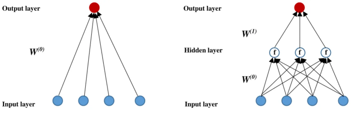
Figure 0. Simple neural network visualizations.
The left figure shows a neural network with no hidden layers, essentially a linear regression. The right figure shows a neural network with one hidden layer (3 nodes). The arrows represent the weights (𝑤𝑖) between signals connecting nodes, and W represents the n-dimensional vector of weights, where n is the number of outputs from the previous layer. In the hidden layer, a nonlinear activation function f transforms the inputs before passing them on to the output.
What enables neural networks to learn nonlinear relations and interactions between predictors is the connectedness of all predictors to the hidden layer nodes and the activation function that is used to transform the aggregated signal before passing it on. Using the right example in Figure 0, the left-most node in the hidden layer transforms its four inputs into an output as:
𝑥1(1) = 𝑓(𝑏(0)+ ∑ 𝑤𝑖(0)𝑥𝑖(0)
4
𝑖=1
)
The output from each node in the hidden layer are then linearly aggregated into the output prediction:
𝑔(𝑥) = 𝑏(1)+ ∑ 𝑤𝑘(1)𝑥𝑘(1)
3
𝑘=1
Applying the same logic to deeper and wider models, the functional form becomes a much more nested function aggregating all weight and bias matrices of each layer and node. This is
Hidden layer
Output layer Output layer
Input layer
f f f
W(0) W(1) W(0)
if x < 0 otherwise
why neural network models are infamously difficult to interpret, unlike a simple linear regression. Machine learning is implemented by adapting the entire collection of weight matrices in order to minimize the error on the training data. The process by which the weights are adapted is called the training algorithm, discussed in detail in the next section, among other parameters that control the regularization of neural networks that are prone to overfitting.
Neural network hyperparameters
Neural network hyperparameters describe the set of topology and regularization technique parameter choices when initializing a neural network. Hyperparameter value choices are non-trivial and “more of an art than science” (Zhang, Patuwo, and Hu (1998)). Thus, neural networks require rigorous optimization through grid search to enable the researcher to find an optimal set of hyperparameter values that work for the specific data in question. In this section I describe the most important hyperparameters analyzed in this paper and defer the description of my grid search process to the next section. The main neural network characteristic choices are activation function, network topology, training algorithm, learning rate, and loss function. The main regularization techniques used are early stopping, dropout, and L1/L2 regularization.
First, the activation function transforms a neuron’s net input signal into a single output signal to be broadcasted further in the network. There are many potential choices for the activation function (such as sigmoid, tanh, rectifier, etc.) (Lantz (2015)). A simple linear activation function with no hidden layers would essentially be an OLS linear regression. One popular example could be the sigmoid function, 𝑓(𝑥) = 1
1+𝑒−𝑥, where the sum of input signals
𝑥, determines an output value in the range of 0 to 1. However, the sigmoid function has fallen out in favor of better performing functions in recent literature, such as the rectifier (Gu et al. (2018)). The R package I use, H2O, offers three popular activation function alternatives: Rectifier, Tanh, and Maxout. The activation function choice is applied to all hidden layers. During hyperparameter tuning, among other variables, I compare the performance of the three activation functions using random grid search, where random combinations of given hyperparameters are used to build different neural network models.
The Rectifier is defined as the positive part of its argument:
𝑓(𝑥) = {0 𝑥
where x is the input to a neuron. It is the most popular activation function as of 2017 (Ramachandran et al. (2017)), and its advantages include 1) computational efficiency through only requiring a max(0,x) function and being capable of outputting true zero values unlike tanh functions, and 2) linear behavior, which makes the network easier to optimize and much less likely to encounter vanishing gradient problems, making the model more stable.
The Tanh is defined as:
𝑓(𝑥) = tanh(𝑥) = 𝑒
𝑥− 𝑒−𝑥
𝑒𝑥+ 𝑒−𝑥
Its benefits include being zero-centered, making it easier to model inputs that may have strongly negative or positive value. Finally, the most recently developed Maxout activation function is defined as:
𝑓(𝑥) = max(𝑤1𝑇𝑥 + 𝑏
1, 𝑤2𝑇𝑥 + 𝑏2)
and is a generalization of the Rectifier. It enjoys the benefits of the Rectifier while fixing the so-called problem of “dying Rectifiers”, where a “dead” neuron always outputs zero for any input for the rest of the training process. The trade-off for Maxout is the doubling of parameters for each neuron, requiring a higher total number of parameters to be trained.
Second, the network topology refers to the chosen structure of number of layers, whether information in the network is allowed to travel backwards, and the number of nodes within each layer. Generally, the larger and more complex networks are capable of identifying more subtle patterns, but for example Gu et al. (2018) show that a network with three layers performs better than one with five layers for stock return prediction with a large set of predictor variables. In my work I use the grid search method that varies the number of layers as well as nodes within each layer, to find the optimal model based on out-of-sample performance. The most commonly used feedforward networks only allow information to flow forwards in a network, and that is the topology I will be using.
Third, the training algorithm refers to the process by which the network is trained using input data. Training a neural network means how the network’s connection weights are adjusted to reflect patterns observed from data. Modern training algorithms are variations on a strategy of back-propagating errors, known simply as backpropagation. In its most general form, backpropagation iterates through many cycles (known as epochs) of two processes, forward and backward phases. In the forward phase an output signal is produced based on the current weights in the network. Then, in the backward phase the error of the output signal compared to the true realized value is propagated backwards in the network to adjust the weights between neurons to reduce future errors. There are many different training algorithms
to choose from, such as the stochastic gradient descent, conjugate gradient or Newton method (Quesada (n.d.)). I use the parallelized stochastic gradient descent offered by the H2O R-package, as it is widely used and fits well with large datasets with many predictor variables. Parallelization drastically improves training time at the cost of result reproducibility (details about controlling for randomness described in Section 4.7).
Finally, for the loss function and learning rate, two important hyperparameters of neural networks, I use the default options that the H2O-package offers: mean squared error (MSE) loss function objective and the adaptive learning rate ADADELTA (Zeiler (2012)). The loss function refers to the minimization objective in backpropagation. The MSE loss function widely used in linear regression is also frequently used in continuous variable predictions in neural networks, measuring and minimizing the inconsistency between predicted values and actual values during training. The learning rate in neural networks refers to the amount parameter weights are updated during training: the higher the learning rate, the faster the model learns, but at the cost of arriving on sub-optimal final weights. Smaller learning rates may allow the model to learn a more optimal set of weights but may take significantly longer to train, or never converge. Various adaptive learning rates have been developed that monitor the model performance during training and adjust the rate in response, which results in generally better performance than manually configured rates. There is no consensus on the best adaptive learning rate to use, but ADADELTA is among the most popular (Goodfellow (2016)). Two ADADELTA learning rate hyperparameters, the time decay factor (rho) and time smoothing factor (epsilon), are tuned through grid search of optimal values.
For regularization techniques, first, early stopping is used to evaluate model skill during training, with user-given stopping rounds n and stopping tolerance p: at regular intervals during training, a value for a chosen scoring metric is calculated, and if this metric hasn’t improved by p in n scoring events, model training is stopped. For example, when a separate validation sample is used, and the stopping metric is R2, the algorithm regularly calculates the pseudo-out-of-sample R2 of the model using the validation sample and uses early stopping if R2 doesn’t improve enough. The important consideration is which data to use in scoring the models during training: in-sample, validation sample (where a specific hold-out sample is used), or cross-validation. I use the H2O-package’s default stopping metric, deviance (similar to mean-squared-error (MSE)) and choose to use a separate hold-out validation sample. The construction of the validation sample was detailed in Section 4.1.
Second, dropout is a regularization technique that generally reduces overfit by randomly dropping out a percentage of nodes in different layers during training. Srinivastava et al. (2014) describe dropout to enable breaking up situations where network layers co-adapt to correct errors from other units, where these co-adaptations do not generalize to unseen data. In my model, different dropout ratios are applied to the input layer and the hidden layers, where common values are around 0.2 for input layers and 0.5 for hidden layers (Srinivastava (2014)). I use the H2O-package default of 0.5 for the hidden layer dropout ratio, but tune the input dropout ratio through grid search.
Third, L1 and L2 regularization prevents neural networks from overfitting by keeping the values of weights and biases small. Both techniques add a regularization term to the loss function, resulting in weight values to decrease. L1 regularization penalizes the absolute sum of weights and can reduce weights to zero, whereas L2 penalizes the squared sum of weights and decays weights towards zero. A regularization parameter determines the strength of L1/L2 regularization and its value is optimized through grid search. Common values for L1 and L2 regularization parameters are small, around 1e-4 to 1e-5. I search for optimal L1/L2 shrinkage parameters through grid search.
Hyperparameter tuning through random grid search
In grid search, the user inputs sets of values for hyperparameters to be considered, and neural network models will be built for each combination of the given hyperparameter values. Then, the out-of-sample performance based on the validation data set can be compared, and the best models selected. Since the hyperparameter set I input is wide (288 combinations), a random grid search (following Bergstra and Bengio (2012)) over a set number of maximum models (150) is performed instead of a cartesian search where all possible combinations are iterated through. To make the results more robust to the randomness caused by parallelized stochastic gradient descent, I repeat this random grid search 10 times before making model choice decisions. This is to counter any lucky or unlucky iterations.
For each model, I calculate the R2 based on the validation data and rank the model from 150 to 1 (150 being the best) for each of the 10 iterations. Then, I separate the results based on the activation function (Rectifier, Maxout, and Tanh). For each hyperparameter value under an activation function, I calculate the average validation R2 and average rank for models that include that hyperparameter value. Then, for each activation function I choose the
hyperparameter values that have the highest average validation R2, confirmed by the average rank that diminishes effects of outliers.
The hyperparameters I test for are hidden layer topology, ADADELTA learning rate time decay factor (rho), ADADELTA learning rate time smoothing factor (epsilon), input dropout ratio, L1 parameter, and L2 parameter. I initially test for the following sets of hyperparameter values resulting in 288 different combinations:
• Activation function: Rectifier, Maxout, and Tanh
• Hidden layers: single-layer 64-nodes, two-layer [64, 32] nodes, three-layer [64, 32, 16] nodes (following the geometric pyramid rule of Masters (1993))
• Rho: 0.9 and 0.99, where 0.99 is the H2O default
• Epsilon: 1e-8 and 1d-9, where 1e-8 is the H2O default
• Input dropout ratio: 0.1 and 0.2, where 0 is the H2O default
• L1: 0 and 1e-4, where 0 is the H2O default
• L2: 0 and 1e-4, where 0 is the H2O default
Based on the results of the above search, I will run a second grid search iteration with incrementally adjusted hyperparameter values to test for improvement. For example, if models with Rho = 0.99 have higher average validation R2 and rank than models with Rho = 0.9, which means a larger Rho seems better, I will adjust the second iteration to test for a larger Rho: Rho = 0.99 and Rho = 0.999.
Controlling for randomness in model training and results through repetition
H2O uses the HOGWILD! (Niu et al. (2011)) scheme to parallelize stochastic gradient descent computation, which drastically speeds up model training, at the cost of reproducibility. As training times without parallelization were unfeasible for practical reasons, using HOGWILD! was a necessity.
Randomness is also an inherent part of machine learning algorithms and particularly neural networks (Brownlee (2016)). Randomness is introduced through the shuffled order of training data, inherent randomness in the algorithms (such as initializing neural network parameter weights with random values), and randomness in data sampling during training (the model trains on random subsets of data at a time). H2O requires setting a seed before beginning training for its random number generator that affects the above three sources of randomness.
Choosing a single seed and reporting only on results produced by that seed would reveal a limited image of prediction performance.
Thus, I repeat hyperparameter grid search 10 times, making model choice decisions based on average R2s, and repeat the resulting three optimized models 100 times each and analyze the mean and standard deviation of their prediction accuracy measures. This also provides an interesting benchmark range of R2 values to compare existing literature on and for future research.
Measuring statistical prediction performance using out-of-sample R2, return correlation and directional accuracy
The main measure of prediction accuracy I use is the out-of-sample 𝑅2. The measure is defined
as: 𝑅𝑜𝑜𝑠2 = 1 −∑ (𝑟𝑖,𝑡+1−𝑓𝑖,𝑡+1) 2 (𝑖,𝑡) ∑ (𝑓𝑖,𝑡+1−𝑟̅ )𝑡 2 (𝑖,𝑡) ,
where 𝑟𝑖,𝑡+1 is the realized return of stock 𝑖 at time 𝑡 + 1, 𝑓𝑖,𝑡+1 is the same stock’s predicted return, and 𝑟̅𝑡 is the historic average return of all stocks in the training sample. Between different subsets of the training sample (e.g. sample that only contains large stocks), the historic average return is calculated separately for each subset. The prediction accuracy is only measured on the testing data set, whose data are not used in model estimation or tuning. In addition, I examine the prediction performance using correlation between predicted the realized returns and percentage of times predicted and realized returns have the same sign (directional accuracy).
Measuring economic value of predictions: Bottom-up equity premium predictions and excess returns from machine learning portfolios
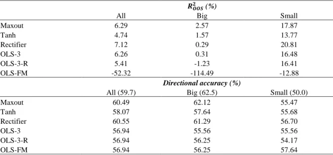
I test the predictive performance of my models in forecasting returns of custom equal-weighted indices of all stocks, largest 500 stocks, and smallest 500 stocks. For this, I construct bottom-up estimates of the index returns using individual stock return predictions of the respective stocks each month. The 𝑅𝑜𝑜𝑠2 metric for this experiment is calculated as the same:
𝑅𝑜𝑜𝑠2 = 1 −
∑𝑇𝑡=1(𝑟𝑡−𝑓𝑡)2 ∑𝑇 (𝑟𝑡−𝑟̅𝑡)2
𝑡=1
where 𝑟̅𝑡 is the historical average return of the index calculated through the training sample time period. These results can then be compared to both the 𝑅2 metric of individual stock return
predictions, and equity premium prediction results like Campbell and Thomson (2008), who estimate the out-of-sample predictability of the S&P 500 index based on several valuation ratios.
Second, I test for the profitability of machine learning long-short portfolios trading all stocks, top 500 largest stocks, and bottom 500 smallest stocks. The portfolios are built by sorting stocks of each respective size category each month based on the individual stock return predictions and buying the top decile stocks and shorting the bottom decile. I then calculate the average monthly returns, volatilities, Sharpe ratios, and the risk-adjusted alphas compared to the Carhart (1997) four-factor model. Trading costs are not considered within the scope of this paper. The results from this test give an idea of the theoretical profitability that could have been realized by investors using the forecasts.
Measuring relative predictor variable importance
To gain insight into relative predictive strength of the predictors, I extract variable importance using the Gedeon (1997) method that H2O has integrated as part of its deep learning functions. The method utilizes the sum of products of normalized weights to evaluate the weight matrices connecting the inputs with the first two hidden layers. I note that evaluating trained neural networks, which are considered “black box” models, is infamously difficult, and many measures of variable importance have been proposed over the years, all riddled with different potential shortcomings (see for example Sarle’s (2000) analysis). The Gedeon method is also applied by Krauss et al. (2017), while Gu et al. (2018) use a simpler measure.
5.
Analysis and results
Hyperparameter grid search results
The first grid search reported in Table 1 reveals a consistent picture of the best-performing parameter values underlined in the table. Across the three models (Rectifier, Maxout, Tanh), the same hyperparameter values seem to be the best fit. Overall, the Rectifier models performed the best in the validation sample with an average R2 of 0.61%, followed by Maxout (0.36%)
and Tanh (0.30%). I note that, on average, the grid search R2 results should appear more positive than in the true out-of-sample test, as the validation sample is a shuffled split from the training sample containing information from the past (as explained in Section 4.1).
Considering the standard deviations reported in brackets, the most unstable model turns out to be Maxout, with an overall average standard deviation of 0.62%. However, it seems the instability is concentrated in models with certain hyperparameter values, such as more than one hidden layer (standard deviations of 0.73% and 0.74%), input dropout of 0.2 (0.73%), L1 of 1.0E-4 (0.80%), so the instability can be avoided through the optimized parameters. The Rectifier models seem equally unstable across parameter values, exhibiting standard deviations of around the average 0.49% against its 0.61% mean R2. The Tanh models display similar behavior, although with lower R2 and standard deviations overall.
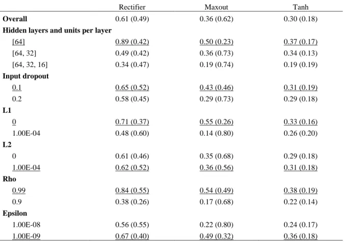
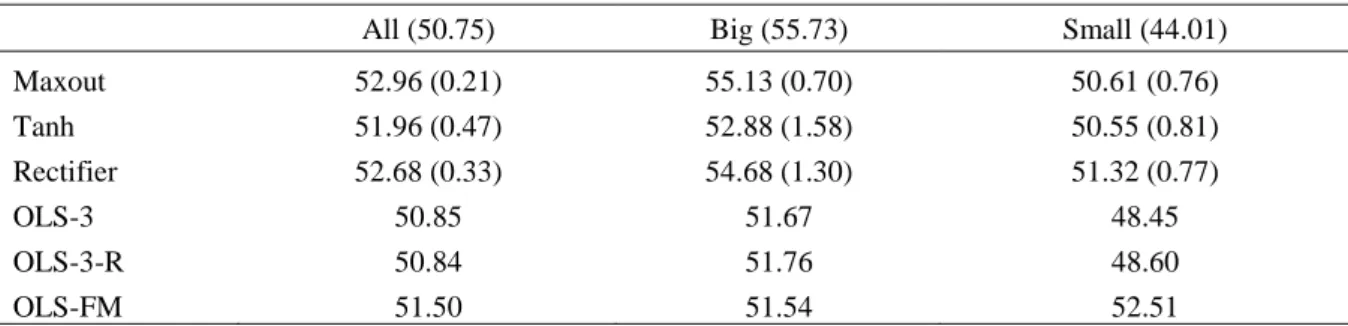
Table 1. Hyperparameter grid search results comparing average validation sample R2 (%) across parameter values. The values reported are average R2 (%) based on the validation data for models including the hyperparameter value defined in the left-most column. Rectifier, Maxout, and Tanh models are compared that differ by their activation function. The random grid search trains 150 models out of 288 possibilities (3 x 3 x 2 x 2 x 2 x 2 x 2), and grid search is repeated 10 times, producing a maximum of 1500 models. 95 models failed in training, and I filter out an additional 18 models with in-sample R2 less than -10%, resulting in a total sample size of 1387 models.
Rectifier Maxout Tanh
Overall 0.61 (0.49) 0.36 (0.62) 0.30 (0.18)
Hidden layers and units per layer
[64] 0.89 (0.42) 0.50 (0.23) 0.37 (0.17) [64, 32] 0.49 (0.42) 0.36 (0.73) 0.34 (0.13) [64, 32, 16] 0.34 (0.47) 0.19 (0.74) 0.19 (0.19) Input dropout 0.1 0.65 (0.52) 0.43 (0.46) 0.31 (0.19) 0.2 0.58 (0.45) 0.29 (0.73) 0.29 (0.18) L1 0 0.71 (0.37) 0.55 (0.26) 0.33 (0.16) 1.00E-04 0.48 (0.60) 0.14 (0.80) 0.26 (0.20) L2 0 0.61 (0.46) 0.35 (0.68) 0.29 (0.18) 1.00E-04 0.62 (0.52) 0.36 (0.56) 0.31 (0.18) Rho 0.99 0.84 (0.55) 0.54 (0.49) 0.38 (0.19) 0.9 0.38 (0.26) 0.17 (0.68) 0.22 (0.14) Epsilon 1.00E-08 0.56 (0.55) 0.22 (0.80) 0.24 (0.17) 1.00E-09 0.67 (0.40) 0.49 (0.32) 0.36 (0.18)
I conduct two iterations of the entire grid search process, where I set each grid to produce 150 models out of the 288 possible combinations, and each iteration to produce 10 grids. The first iteration created 1405 models and the second 1500. The numbers are less than the theoretical 1500 (150 models each grid with 10 grids), because some models become unstable during training fail to complete. I additionally filter away models with in-sample R2 less than -10%, as these can be considered computational failures, and filtering based on in-sample R2 is acceptable prior to engaging in the pseudo out-of-sample validation test. The hyperparameter values tested in the second iterations were adjusted based on the results from the first iteration to further optimize hyperparameter choices. The resulting Table A2 for the second grid search iteration is reported in the Appendix. Overall, changes in activation function, hidden layer topology, and rho had the most significant effects on model performance, while L1, L2 and input dropout were less impactful with models generally working better with smaller regularization parameter values. Based on the second grid search of Table A2, the best-performing models on average chosen for additional performance-testing are shown in Table 2.
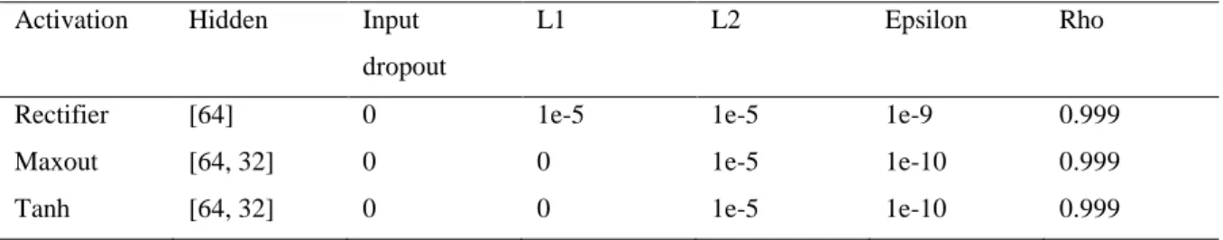
Table 2. Optimized neural network model topologies based on hyperparameter grid search.
“Activation” refers to the activation function of the model, “Hidden” refers to the number of hidden layers and number of nodes within each layer separated by a comma, and “Input dropout” refers to the percentage of inputs randomly dropped out to improve generalization. L1 and L2 refers to the L1- or L2-regularization parameter strength, where a higher value equals more respective regularization. Epsilon is the time smoothing factor and Rho the time decay factor of the ADADELTA adaptive learning rate algorithm used.
Activation Hidden Input
dropout
L1 L2 Epsilon Rho
Rectifier [64] 0 1e-5 1e-5 1e-9 0.999
Maxout [64, 32] 0 0 1e-5 1e-10 0.999
Tanh [64, 32] 0 0 1e-5 1e-10 0.999
Main results: Out-of-sample R2 compared to linear benchmarks
First, I examine the true out-of-sample monthly prediction performance of the three optimized models measured by R2 as defined in Section 4.8. As explained in Section 4.7 about the randomness of separate iterations of the same model, the figures are reported as means accompanied by their standard deviations to give a better picture of average model
performance. Shown in Table 3, the highest out-of-sample statistical prediction performance is achieved by Maxout models, with an average out-of-sample R2 of 0.80%, followed by Tanh models with R2 of 0.39% and Rectifiers with 0.17%. The values are in line with existing literature, such as Gu et al. (2018) who find a monthly out-of-sample R2 of 0.39% on their best-performing rectifier neural network model trained on an extended version of my dataset. The highest individual R2 of all models was 1.07% produced by a Rectifier model, followed by 1.03% by a Maxout model.
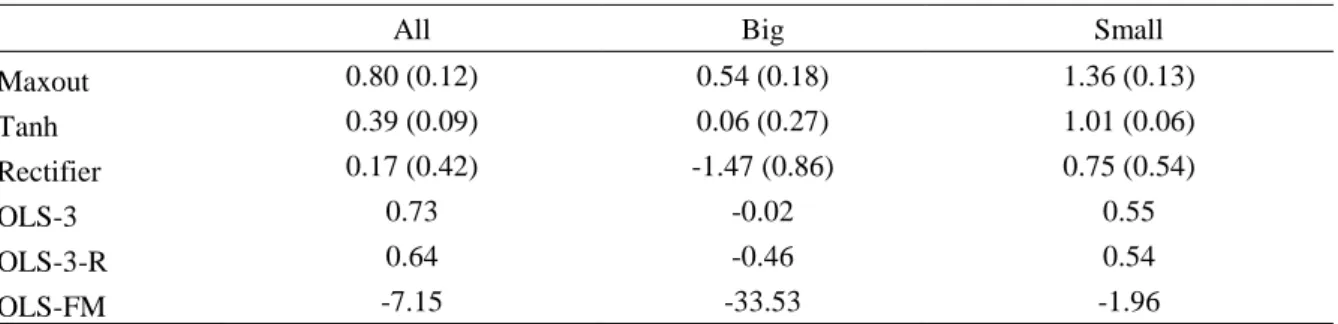
Table 3. Stock-level monthly prediction performance measured by average out-of-sample R2 (%).
The table reports the mean out-of-sample R2 (%) and the standard deviations of R2 results (in brackets) from repeating model training and prediction 100 times for the three neural network models (Rectifier, Maxout, Tanh), and compares them to the OLS benchmark using lagged market return, firm size, book-to-market, and momentum (OLS-3), OLS-3 with annual refitting (OLS-3-R), and Fama and French (2006) OLS (OLS-FM) that uses coefficient estimates from monthly cross-sectional regressions on OLS-3 predictors except market return to predict next month returns. Results are also reported for subsamples that include only the top 500 (Big) and bottom 500 (Small) stocks by market value (models built on full data, predictions subsampled).
All Big Small
Maxout 0.80 (0.12) 0.54 (0.18) 1.36 (0.13) Tanh 0.39 (0.09) 0.06 (0.27) 1.01 (0.06) Rectifier 0.17 (0.42) -1.47 (0.86) 0.75 (0.54) OLS-3 0.73 -0.02 0.55 OLS-3-R 0.64 -0.46 0.54 OLS-FM -7.15 -33.53 -1.96
In addition, I analyze prediction performance in the largest and smallest stocks by market value. This is done by calculating the R2 using returns of only the top 500 and bottom 500 stocks by market value each month, subset from existing predicted returns produced by models trained on the full data. Table 3 shows that neural network predictions are generally better in small stocks and worse in large stocks: all R2 in the “All” category are less than those in “Small” and
greater than those in “Big”. For the linear benchmarks, overall predictions on all stocks performed the best, followed by small stock predictions. This confirms there are differences in the return predictability of small versus large stocks and indicates that the neural networks fit more towards small stocks’ rather than large stocks’ return behavior, which seems reasonable as a majority of stocks in the U.S. market data belongs to small stocks.
The high small stock performance is in line with existing research that find return predictability to be the strongest among stocks with the highest levels of arbitrage frictions or
high trading costs (Lesmond, Schill, and Zhou (2004), Hou and Moskowitz (2005), Chordia, Roll, and Subrahmanyam (2008), Li and Zhang (2010), and Lam and Wei (2011)). My findings also confirm Green et al.’s (2017) observation that anomalies are mostly present in microcap stocks and not robustly so in all stocks. The result contradicts those of Gu et al. (2018), who find that predictions by neural networks are the most accurate in the top 1000 stocks (0.72% at best), then the bottom 1000 stocks (0.46% at best), then all stocks (0.39% at best). The differences are most likely to stem from data and algorithm differences. Gu et al. train their models on data from 1957 to 1986, include more macroeconomic predictors, and conduct out-of-sample testing on data from 1987 to 2016. A deeper investigation into the reasons behind the result differences is beyond the scope of this paper.
Comparing the results to the three linear regression benchmarks, neural networks do not universally outperform the linear benchmarks. The worst-performing OLS-FM, which cannot use lagged market return as a predictor in its monthly cross-sectional regressions, underperforms all other models significantly, with an OOS R2 of -7.15%. The other two,
OLS-3 and OLS-OLS-3-R, which both include lagged market return as a predictor in their panel regressions, outperform Tanh and Rectifier models on average. Both the neural networks and the OLS regressions heavily use the lagged market return as the most important predictor, shown more evidently in Section 5.8 about variable importances. So, a linear model using a longer training sample without annual refitting seems to generalize well into the bull-market period of 2009-2018. The linear benchmarks also perform worse in big stocks. For small stocks, the results are worse than for all stocks, which could imply that the models fit more towards average-sized stocks, and that neural networks are better able to learn the anomalies in small stocks.
Standard deviations of out-of-sample R2 and correlation between in-sample and out-of-sample performance
The standard deviations vary between the models and the stock size categories. Overall, the Rectifier models seem to be the most unstable, with the highest standard deviations across size categories. For example, the Rectifier has a standard deviation of 0.42% for all stocks, against a mean of 0.17%, whereas the Maxout has a standard deviation of 0.12% against a mean of 0.80%. Figure 1 presents a visualization of the variance in results, plotting the percentage frequency distribution of out-of-sample (OOS) R2 results. The graph shows the high variance
of Rectifier model results, with R2 values almost uniformly spread across the entire range, and the relatively more stable performance of the Maxout and Tanh models. Tanh models in particular center densely around the 0.4% mean, with 38% of R2 results between 0.3% and 0.4%. The variance is further visualized in the scatterplot of Figure 2.
Figure 1. Frequency distribution of out-of-sample R2s of three neural network models iterated 100 times. Three neural network models are used to predict monthly excess stock returns. Each model is repeated 100 times with its prediction performance measured by out-of-sample R2 recorded. The graph shows the frequency distribution of the resulting 100 R2s for each model, distinguished by the three different lines. The x-axis describes the R2 value ranges, and the y-axis the percentage of results in that value range.
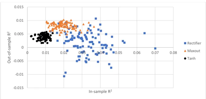
The correlation between in-sample R2 and out-of-sample R2 is -28.9% for all results, -15.8% for Rectifier model results, -12.6% for Maxout results, and 8.1% for Tanh results. From Figure 2 we see that the overall negative correlation is driven by the strong in-sample performance of some rectifier models and their relatively poor out-of-sample performance, as well as the strong out-of-sample performance of the Maxout models. The Rectifier’s negative correlation is mainly driven by the models with very strong in-sample but poor out-of-sample performance, suggesting Rectifiers more easily overfit for the noisy data being unable to generalize out-of-sample. The Maxout and Tanh models are more stable and produce denser scatters on the graph. The scatterplot also shows the average outperformance of Maxout compared to the other two models, with its scatter almost entirely above Tanh results, and on average above the high-variance Rectifier results.
0% 5% 10% 15% 20% 25% 30% 35% 40% <-0.4% -0.3% -0.2% -0.1% 0% 0.1% 0.2% 0.3% 0.4% 0.5% 0.6% 0.7% 0.8% 0.9% >0.9% Fre q u en cy Out-of-sample R2range Rectifier Maxout Tanh
Figure 2. Scatterplot of in-sample versus out-of-sample R2 for the three optimized models.
The x-axis is the in-sample R2, and y-axis the out-of-sample R2 from the selected model performance test where 100 of each model are trained and tested on out-of-sample data.
Rolling past 12-month out-of-sample R2 over time
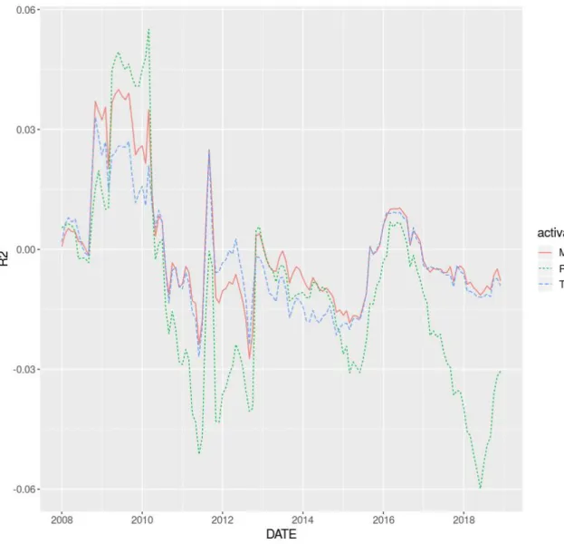
Figure 3 plots the rolling 12-month out-of-sample R2 over the testing period (2007-2018). The graph provides information on the temporal development of the R2 results. Overall, the models follow the same trends with peaks and troughs at roughly the same time. Maxout and Tanh models align very closely, while Rectifiers are generally lower. It seems that the accuracy of predictions measured by R2 varies greatly over time, peaking during 2009-2010 and bottoming during 2011-2013. At a surface level analysis, there seem to be indications of greater prediction accuracies during times of higher volatility as measured by the CBOE Volatility Index (VIX). For example, during the R2 peaks of 2009-2010, 2011-2012, 2015-2016 and end of 2018, the VIX also displays spikes in its level3 roughly during these times. The findings are somewhat surprising, considering the models’ reliance on the market return predictor (discussed in Section 5.8), and the understanding in literature that, for example, momentum strategies perform poorly during high market volatility (Wang and Xu (2015)). One might expect models to perform the best during low volatility periods when stocks follow a similar trend, but the temporal results of Figure 3 reveal that the neural networks perform particularly well during market turbulence. One explanation could lie in the out-of-sample R2 measure itself, where
3 See VIX levels for example at Yahoo Finance for the time period 2007-2018. -0.015 -0.01 -0.005 0 0.005 0.01 0.015 0 0.01 0.02 0.03 0.04 0.05 0.06 0.07 0.08 Ou t-of -s amp le R 2 In-sample R2 Rectifier Maxout Tanh
during turbulent times the historical average becomes a worse predictor, and the neural network predictions are able to better predict differences. During calmer periods the historical average serves as a solid predictor, and neural networks may introduce unnecessary variation in predictions. There may be many other reasons why out-of-sample R2 varies over time, but I leave a deeper investigation into the temporal development of R2 to future research.
Figure 3. Rolling past 12-month out-of-sample R2 over the testing period.
The figure plots the rolling past 12-month out-of-sample R2 over the testing period 2007-2018, with the first value being January 2008 and its out-of-sample R2 based on the past 12-months of predictions. The three different lines represent the three neural networks, Maxout, Rectifier, and Tanh. The x-axis represents the date, and the y-axis the R2.