Published by Canadian Center of Science and Education
Dynamic Quantile Panel Data Analysis of Stock Returns Predictability
Bülent Güloğlu1, Sinem Güler Kangalli Uyar2 & Umut Uyar31 Department of Economics, Istanbul Technical University, Macka, Istanbul, Turkey 2 Department of Econometrics, Pamukkale University, Kinikli, Denizli, Turkey
3 Department of Business Administration, Pamukkale University, Kinikli, Denizli, Turkey
Correspondence: Umut Uyar, Dr., Department of Business Administration, Pamukkale University, Kinikli, Denizli, Turkey. E-mail: [email protected]
Received: November 25, 2015 Accepted: December 30, 2015 Online Published: January 25, 2016 doi:10.5539/ijef.v8n2p115 URL: http://dx.doi.org/10.5539/ijef.v8n2p115
Abstract
This paper analyses the effect of financial ratios on stock returns using quantile regression for dynamic panel data with fixed effects. Eighty three firms of manufacturing industry, which were traded on the Borsa Istanbul for 2000-2014 period, are covered in the study. The most of financial variables have heterogeneous structure so they generally include extreme values. Thus, panel quantile regression technique, suggested by Koenker (2004), is used. Since the technique yields robust estimator in the case of extreme values the Gaussian estimators will be biased and not efficient. The sensitivity of relationship, on the other hand, can be studied for different parts of the stock returns’ conditional distribution by using quantile regression technique. However, because of that the lagged of dependent variable is used as an explanatory variable in dynamic panel models, fixed effect estimators will be biased. Thereby, in this study the instrumental variable approach suggested by Chernozhukov and Hansen (2006) is used to produce unbiased and consistent estimators.
The results show that the stock returns respond to the changes on the financial leverage ratio, the dividend yield, the market-to-book value ratio, financial beta and the total active profitability variables differently for the different parts of the stock returns’ conditional distribution. They also indicate that, at high quantiles, return fluctuations in the current period will be more effective for investors’ transaction attitudes on stocks for the next period.
Keywords: efficient market hypothesis, financial ratios, quantile regression instrumental variable approach, dynamic panel
1. Introduction
The most significant parameter in the stock market which influences investors’ decision is stock price movement. Having more developed and stable stock market depends on investors’ decisions while correctness of those decisions depends on determination of factors correctly and sensibly that are affecting stock prices.
Whether the possibility of making fortune out of estimation of future stock prices by analyzing historical stock price data exists or not has been the main focus of many studies in the literature. As a result of the studies on stock price, “Efficient Market Hypothesis” has emerged. According to the Efficient Market Hypothesis, it is not possible to make abnormal money by estimating future stock prices by analyzing its prices in the past. However, it is also quite hard to reach a certain decree about the efficiency of the market. It is neither completely efficient nor not. If new information arrive to the market and then stock prices react so fast to this information, it can be said notionally that the market is efficient otherwise, it can not be considered efficient. The efficient market hypothesis must be tested to see if stock prices or their returns can be estimated or not. However, efficient market hypothesis can not be tested by itself, it must be tested certainly together with another assumption. Hence, efficiency mostly takes place by testing jointly a model which is determining the returns on stock prices. In this study, validity of the efficiency hypothesis was tested by means of an econometric model investigating the relationship between stock price returns and financial ratios. What we have aimed is to decide that what type of market the stock market of manufacturing industry of Borsa Istanbul is in terms of efficiency. Besides based on the assumption of companies have different financial structures, it will also be investigated that how the relationship between return on a stock and financial ratios changes according to the different parts of distribution of returns on a stock.
One of the problems observed in the studies which are conducted based on data set consisting financial ratios of companies is the extreme value problem. When this problem arises, either extreme values are ignored or these values are discarded. In the case that the distributions of error terms are not normal and there are extreme values, Gaussian model estimators that are used commonly during the investigation of the relationship between variables, are generally biased and not efficient. In this case, it is required to be used more robust estimators. The relationship between financial ratios and returns on stocks was investigated by panel quantile regression analysis recommended by Koenker (2004) which is less sensitive toward heteroscedasticity and extreme values compared to Gaussian models. Accordingly, financial ratios’ (leverage rate, total return on assets, dividend yield, and market value/book value) effects on stock prices for 83 companies whose stocks were being traded within the manufacturing industry in BIST-100 in the period of 2000-2014 were analyzed by employing dynamic panel quantile regression with fixed effects.
In addition to the financial ratios, the lag of stock returns was also included into the model as an explanatory variable. The basic rationale under this relies on “state dependence effect” proposed by Heckman (1981a). According to this proposal, individuals who had faced with a certain condition/situation and obtain some information and experience out of it in past, use this information/experience when they experience similar or same cases in future. State dependence effect can be considered for the investors who prefer to make investment on stocks, investors can decide whether to make investment on a certain stock or not by analyzing price movements in the past. Hence, when there is a price fall in a stock’s price in previous period, demand for this stock is supposed to be increased in current period. On the contrary, the demand is supposed to be decreased. In other words, historical stock data can be effective on investor behaviors in current or future periods. In the analysis along with this angle, stock returns’ previous period effect was also taken into consideration. However, in case of that there are the lags of dependent variable as explanatory variables in panel data models with fixed effects, the fixed effects estimator generally are biased. Anderson and Hsiao (1981, 1982) and Arellano & Bond (1991) have shown that this bias can be removed in dynamic panel data models through instrumental variable approach.
Antonio F. Galvao Jr. (2011) investigated that forecasting performance of dynamic panel quantile regression model with fixed effects in his article. The author showed that fixed effects estimators can be biased in case there are the lags of dependent variables in the panel data model an explanatory variables and used Chernozhukov and Hansen (2006)’s quantile regression-instrumental variables method in which the lags of explanatory variables are taken as instrumental variables to reduce this dynamic bias. Monte Carlo simulations have shown that how the instrumental variable approach reduced the dynamic bias acutely and how the empirical levels came up so close to the theoretical levels for the prediction intervals. As a result of the study, a case study covering an application of estimation of 18 OECD countries’ growth rate was included. In their study, Harding and Lamarche (2009) compared performances of the least squares estimators and quantile regression estimators. They used quantile regression approach in the panel data models including endogeneous variables and explanatory variables relevant with individual effects.
This study scrutinizes the determinants of stock returns for the stocks listed at Borsa Istanbul 100 index (BIST-100). To get a better understanding of the predictability of stock returns we adopt a dynamic approach and use a dynamic panel quantile regression model. Quantile regression model has two advantageous over the standard regression model. First unlike the standard regression model which explains the conditional mean of dependent variable, quantile regression allows us to create entire distribution of dependent variable and thus gives a more complete picture of the relationship between dependent and explanatory variables without segmenting the sample. Second, while standard regression restricts the effect of an explanatory variable for example, profitability to be same for all companies on stock returns, quantile regression technique permits us to explore the effects of profitability on high and low stock returns. Third quantile regression produces estimations which are more robust to outlying observations on the dependent variable (Mello & Perrelli, 2003). This turns out to be quite important since returns on financial assets display erratic behaviour, in the sense that large outlying observations occur with rather high-frequency (Franses & Dijk, 2003, p. 5).
2. Literature
The predictability of stock returns using financial ratios has been long debated among the researchers. Earlier studies conducted by Sharp (1964), Lintner (1965) and Mossin (1966) attempted to explain expected returns by systematic market risk. Within the framework of CAPM they showed that expected stock returns are positively and linearly related to market risk. However as argued by Artmann et al. (2012) has lost credibility as its predictive power was found very poor in many empirical studies. Starting with Basu (1977, 1983) many authors showed that a firm’s size, earning to price ratio, book to market equity ratio, leverage, profitability, dividend
yields and lagged stock returns are important predictors of stock returns. Fama and French (1988) examined that ability of dividend yields to predict stock returns and they found that the degree of forecasting stock returns by dividend yield increases with return horizon; their tests confirmed that the predictable component of return is a small fraction of short–horizon return variance.
Hodrick (1992) examined that predictability of long-horizon stock returns using dividend yields and obtained a strong evidence for the predictive power of one-month-ahead returns at least for the sample from 1952 to 1987. He showed that changes in dividend yields forecast significant persistent changes in expected stock returns. Fama and French (1992) documented a significant relationship between firm size, book-to-market ratios and security returns for nonfinancial firms. However, Barber and Lyon (1997) argued that relationship among firm size, book-to-market ratios, and security returns is similar for financial and nonfinancial firms. Kothari and Shanken (1997) used Bayesian-bootstrap simulation in estimating likelihood of different slope values on the historical OLS estimates, they also used univariate least square technique (OLS) to measure the predictive power of dividend yield. Both of conventional and bootstrap methods, confirmed the existence of dividend yield predictability for the value- and equally-weighted returns. They found that the book-to-market ratio has also predictive power in both cross-section and time-series excess returns.
Lewellen (2004) studied if financial ratios like dividend yield can predict aggregate stock returns. He showed that dividend yield predicts market returns during period 1946-2000, as well as in various subsamples and book-to-market and the earnings-price ratio predict returns during 1963-2000 being shorter sample. Campbell and Yogo (2006) stressed that conventional t test of predictability of stock returns could be biased towards to reject the null too frequently when the predictor variable is persistent and its shocks are correlated with stock returns. After showing that standard t test leads to misleading inferences, they advanced an efficient test which overcomes this shortcoming of standard t test. Using the efficient test they found evidence for the predictability of stock returns using dividend–price and smoothed earning-price ratios. However, they indicated that the dividend-price ratio predicts returns only at annual frequencies.
Ang and Bekaert (2007) examined the predictive power of the dividend yields for forecasting excess returns, cash flows and interest rates. They found that dividend yields predict excess returns only at short horizons together with the short rate and do not have any long-horizon predictive power. Jiang and Lee (2007) proposed a loglinear cointegration model, which accounts for potential cointegration and explains future profitability and excess stock returns in terms of a linear combination of log book-to-market and log dividend yield by extending Campbell and Shiller’s (1987) and Vuolteenaho’s models (2000, 2002). This model takes into account possible non-stationarity of these variables. They showed that the loglinear cointegration model performs better than either the log dividend yield model or the log book-to-market model in terms of cross-equation restrictions tests, excess return forecasting performance, and out-of-sample forecasting performance comparisons.
Bhandri (1988), showed that a significant effect of the leverage ratio on stock returns. Fama and French (1992) also examined the effect of leverage ratio on the stock returns and they made two different definitions for the leverage ratio. In the first, the leverage was defined as the ratio of book assets to market equity, while in the second the ratio of book assets to book equity. More interestingly, they found that the leverage ratio had a positive relation with the stock returns by using the first definition while they obtained a negative effect of leverage on stock returns by using the second definition.
Lam (2002) investigated also the relation between the leverage ratio and the stock returns using two different definitions for the leverage ratio such as book leverage and market leverage. He found that both of two leverage ratios have explanation power on the stock returns. Johnson (2004) developed an option-based value of the firm in the presence of information risk (measured by analyst forecast dispersion). He found a weak unconditional positive relation between leverage and future returns, but after controlling for underlying firm characteristics (e.g., volatility) he showed that the relation between leverage and future returns turned out to be negative. Haugen and Baker (1996) and Cohen et al. (2002) found that more profitable firms have higher average stock returns, while Fairfield, Whisenant, and Yohn (2003) and Titmanet al. (2004) showed that firms investing more tend to have lower stock returns. Fama and French (2008) studied anomalies associated with stock returns and profitability. They found that among profitable firms, having higher profitability tend to have abnormal high returns, but they argue that there is little evidence that unprofitable firms have unusually low returns. Timmerman and Cenesizoglu (2008), explored the predictability of stock returns in a quantile regression framework and considered if a range of economic state variables are helpful in predicting different quantiles of stock returns representing left tails, right tails or shoulders of the return distribution. They found that many variables have an asymmetric effect on the return distribution.
Kheradyar, et al. (2011) investigated whether or not financial ratios can predict stock returns for period from January 2000 to December 2009 in Malaysia stock exchange. By using three financial ratios including dividend yield, earning yield and book-to-market ratio, they showed that the financial ratios can predict stock return and yet, the book-to-market ratio has higher predictive power than dividend yield and earning yield respectively. Furthermore, they found that the financial ratios are able to enhance stock return predictability when the ratios are combined in the multiple predictive regression models. Bali et al. (2008) undertook an analysis of the predictability of stock returns by using market-industry-level and firm-level earnings. They concluded that neither dividend payout ratio nor the level of aggregate earnings can forecast the excess market return.
Aktas (2008) examined the relationship between stock returns and financial ratios for medium-term. The reason for using medium-term is to support investment strategies especially for the medium and long term funds such as pension and insurance funds. The results illustrated that acid test and cash flows from operation activities divided by equity ratios are suitable for 1995-1999 and gross profit divided by sales and net profit divided by sales ratios are suitable for 2003-2006. Hjalmarsson (2010) tested for stock return predictability in the largest and most comprehensive data set analyzed so far, using four common financial variables: dividend-price (DP) and earnings price (EP) ratios, short interest rate, and term spread. The data used in that study contain over 20,000 monthly observations from 40 international markets including 24 developed and 16 emerging economies. In addition, he developed new methods for predictive regressions with panel data and showed that inferences based on the standard fixed effects estimator suffer from severe size distortions in the typical stock return regression. So he proposed an alternative robust estimator. The finding of empirical part of the study indicate that the short interest rate and the term spread are fairly robust predictors of stock returns in developed markets. In contrast, no strong or consistent evidence of predictability is found when considering the EP and DP ratios as predictors. Caglayan and Kangalli (2011) analyzed the effect of macroeconomic factors on stock returns using static and dynamic models for binary panel data. Eighty four firms of manufacturing industry, which are traded on the Borsa Istanbul, are covered in the study. The results show that inflation rate, interest rate, exchange rate and balance of trade deficit have significant effects on stock returns. They also indicate that price fluctuations in previous period will affect transaction attitudes of investors on stocks in current period.
Using two different models Nargelecekenler (2011) investigated that relationship between price/earnings ratio and stock prices for a panel of 24 sectoral index over the 2000-2008 period in Borsa Istanbul. He used one-way fixed effects models and tested for low price/earnings ratio effect. The results, provided evidence for the existence of low price/earnings ratio effect is all but metal goods industry. Aydemir et al. (2012) studied if the financial ratios are effective in determining stock prices. Using a panel data set covering 73 manufacturing companies listed in Borsa Istanbul over the period of 1990-2000. He showed that profitability and liquidity ratios have a positive effect on stock returns. Moreover, leverage ratio which is taken as an indicator of indebtedness has the same effect. However, he also showed that operating ratios have no impact on stock returns. Korkmaz and Karaca (2013) analyzed the factors affecting stock returns using a panel of 16 companies listed in Borsa Istanbul for period 1998-2010. Among the variables which are likely to affect the stock returns such as Dividend Payout Ratio, Earnings Per Share, Return on Assets, Market to Book value, change in Market value of firm, only earning per share and change in firm’s market value were reported to affect positively and significantly the stock returns.
3. Data and Methodology
Since the study of Koenker and Bassett (1978), quantile regression technique has been widely used in empirical studies. The idea that the effects of right hand side variables are the same across the quantiles of the response variable may be restrictive. As mentioned by Mello and Perrelli (2003) explanatory variables can affect the dispersion, skewness, stretch one tail, fatten the other etc. In those cases the conditional distribution of dependent variable can be affected and standard regression technique which estimates conditional mean of dependent variable turns out be inappropriate. The main difference between standard and quantile regression lies in the weighting schemes. While standard regression minimizes unweighted sum of squared residuals, quantile regression minimizes the weighted sum of the absolute value of residuals.
In this study we use a dynamic quantile regression model to allow for the effects of past stock returns, which have been well documented in the earlier studies. We consider the following dynamic quantile panel regression:
𝑄𝑙𝑟𝑒𝑡𝑢𝑟𝑛𝑠𝑖𝑡(𝜏|𝑋𝑖𝑡) = 𝛽1(𝜏)(𝑙𝑟𝑒𝑡𝑢𝑟𝑛𝑖,𝑡−1) + 𝛽2(𝜏)(𝑙𝑒𝑣𝑒𝑟𝑎𝑔𝑒𝑖𝑡) + 𝛽3(𝜏)(𝑝𝑟𝑜𝑓𝑖𝑡𝑎𝑏𝑖𝑙𝑖𝑡𝑦𝑖𝑡) + 𝛽4(𝜏)(𝑑𝑦𝑖𝑒𝑙𝑑𝑖𝑡) +
𝛽5(𝜏)(𝑚𝑣_𝑏𝑣𝑖𝑡) + 𝛽6(𝜏)(𝑏𝑒𝑡𝑎) + 𝛼𝑖+ 𝑢𝑖𝑡 (1) where lreturn is stock returns, leverage is financial leverage, profitability is total active profitability, dyield is
dividend yield, mv_bv is the ratio of market value to book value, beta is financial beta coefficient measuring systematic risk, and finally i represent individual effects which are assumed to be fixed in the study. Data covers 83 manufacturing firms listed at Borsa Istanbul 100 index (BIST-100) and spans the annual period from 2000 to 2014. We exclude the stocks that did not survive during the overall period and thus obtain a balanced panel of 83 firms. All data was obtained from BIST-100 web site and Bloomberg.
4. Findings
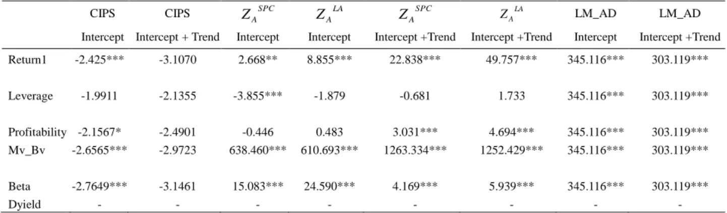
Before examining the relationship between returns on stock and financial ratios, the existence of extreme values were investigated by means of descriptive statistics and kernel density function. The existence of extreme values and the fact that the distribution of error terms is not normal were presented. Since there are extreme values and normal distribution assumption is not valid, Gaussian fixed effect estimators will be biased (Koenker, 2004). In this case, quantile regression method which is less sensitive toward the extreme values compared to the models based on Gaussian conditions in the analysis.
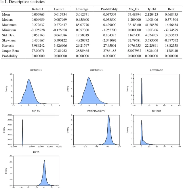
Before the estimation of models, descriptive statistics used in the investigation of existence of the extreme values and normal distribution of error terms were exhibited in Table 1. Figure 1 presents kernel density functions (Note 1).
Table 1. Descriptive statistics
Return1 Lreturn1 Leverage Profitability Mv_Bv Dyield Beta Mean 0.006963 0.015734 3.012371 0.037307 37.48394 2.120423 0.668435 Median 0.004959 0.007969 0.455600 0.038500 1.209000 1.00E-06 0.571504 Maximum 0.272637 0.272637 85.07770 0.429000 38183.60 41.28530 16.56654 Minimum -0.125928 -0.125928 0.057300 -1.252700 0.000000 1.00E-06 -32.74579 Std. Dev. 0.052163 0.062086 12.58319 0.104325 1162.431 4.024205 3.053633 Skewness 0.430167 0.590122 4.920372 -2.341092 32.79681 3.583060 -0.377572 Kurtosis 3.986242 3.426906 26.21797 27.45001 1076.753 22.25891 18.82558 Jarque-Bera 77.00671 70.81952 28589.65 27861.83 52027932 18984.05 11285.40 Probability 0.000000 0.000000 0.000000 0.000000 0.000000 0.000000 0.000000
Figure 1. Kernel density functions 0 2 4 6 8 10 -.2 -.1 .0 .1 .2 .3 .4 D en si ty RETURN1 0 2 4 6 8 -.2 -.1 .0 .1 .2 .3 .4 D en si ty LRETURN1 .0 .1 .2 .3 .4 .5 .6 .7 -20 0 20 40 60 80 100 D en si ty LEVERAGE .0000 .0005 .0010 .0015 .0020 .0025 .0030 -10,000 0 10,000 20,000 30,000 40,000 D en si ty MV_BV 0 1 2 3 4 5 6 -1.5 -1.0 -0.5 0.0 0.5 D en si ty PROFITABILITY .0 .1 .2 .3 .4 .5 -10 0 10 20 30 40 50 D en si ty DY IELD .00 .05 .10 .15 .20 .25 -40 -30 -20 -10 0 10 20 D en si ty BETA
The time series properties of data used in this study have been analyzed using the CIPS panel unit root test (Pesaran, 2007) and ZSA ZLA tests (Hadri-Kuruzomi, 2012) panel unit root tests and Durbin-H panel cointegration test (Westerlund, 2008) as well. Using these second order generation tests has been justified since the LM_AD statistics strongly reject the absence of cross section dependence (Table 2).
Table 2. Second generation panel unit root tests
CIPS Intercept CIPS Intercept + Trend SPC A Z Intercept LA A Z Intercept SPC A Z Intercept +Trend LA A Z Intercept +Trend LM_AD Intercept LM_AD Intercept +Trend Return1 -2.425*** -3.1070 2.668** 8.855*** 22.838*** 49.757*** 345.116*** 303.119*** Leverage -1.9911 -2.1355 -3.855*** -1.879 -0.681 1.733 345.116*** 303.119*** Profitability -2.1567* -2.4901 -0.446 0.483 3.031*** 4.694*** 345.116*** 303.119*** Mv_Bv -2.6565*** -2.9723 638.460*** 610.693*** 1263.334*** 1252.429*** 345.116*** 303.119*** Beta -2.7649*** -3.1461 15.083*** 24.590*** 4.169*** 5.939*** 345.116*** 303.119*** Dyield - - - -
Note. *** % 1 level of significance, ** %5 level of significance, * %10 level of significance.
The CIPS and ZSA tests statistics illustrated in Table 2 give mixed results about the order of integration of variables. When the CIPS test fail to reject unit root hypothesis, the ZSA and ZLA tests also fail to reject the stationarity hypothesis.
These findings lead us to using the Durbin-H statistic which does not require the series to have the same order of integration when testing for cointegration. The test results are illustrated in Table 3. Accordingly the null of cointegration is rejected at 1% level of significance. Since the series seem to be cointegrated we turn to estimation.
Table 3. Durbin-H panel cointegration test results
Test Statistics Probability Value Durbin-H Group Statistic 13.080 0.000
Durbin-H Panel Statistic 8.858 0.000
5. Estimation Method
Estimation of quantile dynamic panel fixed effects model such as in equation 1 could be carried out using a general approach recently introduced by Koenker (2004). However this can produce bias in the estimates as seen in the least squares case when time dimension is not large enough. As argued by Galvao (2011), differencing or within transformation of model 1 is not appropriate in this case since this can alter in a fundamental way what is being estimated. Inspired from Chernozhukov and Hansen (2006), Galvao (2011) suggests the use of instrumental variable quantile regression method to reduce the dynamic bias. The novel approach developed by Galvao (2011) combines conventional dynamic panel data approach and quantile instrumental variable approach. The main advantage of this approach is that it does not require any transformation of the model.
We estimate equation 1 using the lagged values of dependent variable as instruments as suggested by Galvao. The estimation results are shown in Table 4.
Table 4. Estimation results
Quantile constant lreturn1 leverage profitability dyield mv_bv Beta 5th -0.0297*** -0.2221*** 0.0007*** 0.1405*** -0.0022*** 4.40e-06*** 0.0011*** 10th -0.0275*** -0.2176*** 0.0010*** 0.1459*** -0.0023*** 4.13e-06*** 0.0016*** 25th -0.0130*** -0.2313*** 0.0009*** 0.1492*** -0.0029*** 3.75e-06*** 0.0026*** 50th 0.0042*** -0.1934*** 0.0008*** 0.0858*** -0.0029*** 2.93e-06*** 0.0024*** 75th 0.0542*** -0.2289*** 0.0008*** 0.0652*** -0.0035*** 2.13e-06 *** 0.0336*** 95th 0.0679*** -0.3132*** 0.0006*** 0.0835*** -0.0046*** 1.47e-06 *** -0.0003*** Pooled OLS 0.0091*** -0.1885*** 0.0008*** 0.0839*** -0.0027*** 2.85e-06** 0.0013*** Fixed-Effects 0.0098*** -0.2123*** 0.0008*** 0.0928*** -0.0029*** 2.56e-06* 0.0013***
Pseduo-R2 0.2354 (5th) 0.1861 (10th) 0.1548 (25th) 0.1361 (50th) 0.1699 (75th) 0.2987 (95th) - Wald-F 134.7045*** 83.2819*** 71.62820*** 47.23795*** 37.43145*** 23.1399*** - Wald chi-square 808.2273*** 499.6911*** 429.7692*** 283.4277*** 224.5887*** 138.8395*** -
Note. *** % 1 level of significance, ** %5 level of significance, * %10 level of significance.
If Table 4 is analyzed, it can be seen that coefficients of all variables and constant terms as well, are statistically significant at 1% in quantile regression models. When the coefficients of variables were evaluated, it can be seen that coefficient values for each quantile vary and their signs change for some variables. In other words, stock returns react differently against the changes in financial ratios for the different points of conditional distribution of returns. This may be result of different financial conditions of companies. Furthermore, the values of pseduo-R2 present the explanation level of quantile regression model changing for each quantile.
In case the model was estimated by pooled OLS method, it can be seen that except the constant term and dividend yield variable, all rest of the variables’ coefficients are statistically insignificant for all significance levels. In the fixed effect estimation of the model while profitability variable has 5% significance level, dividend yield (dyield) has 1% significance level and rest of the variables are statistically insignificant.
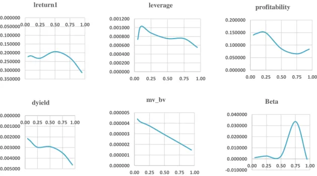
The values of the coefficients associated with each explanatory variable across different quantiles are illustrated in Figure 2. As seen the values of the coefficients vary across quantiles. These variations seem significant as the equality of coefficients across different quantiles has been rejected by Wald Chi-Square test.
Figure 2. Relationships between return on stocks and financial variables for different quantiles
On the graph that belongs to the variable of lreturn1, we can see that effect of the stock returns in the previous period is more negative at higher quantiles compared to the current period because of the short-term sales for
-0.350000 -0.300000 -0.250000 -0.200000 -0.150000 -0.100000 -0.050000 0.000000 0.00 0.25 0.50 0.75 1.00 lreturn1 0.000000 0.000200 0.000400 0.000600 0.000800 0.001000 0.001200 0.00 0.25 0.50 0.75 1.00 leverage 0.000000 0.050000 0.100000 0.150000 0.200000 0.00 0.25 0.50 0.75 1.00 profitability -0.005000 -0.004000 -0.003000 -0.002000 -0.001000 0.000000 0.00 0.25 0.50 0.75 1.00 dyield 0.000000 0.000001 0.000002 0.000003 0.000004 0.000005 0.00 0.25 0.50 0.75 1.00 mv_bv -0.010000 0.000000 0.010000 0.020000 0.030000 0.040000 0.00 0.25 0.50 0.75 1.00 Beta
profit. In other words, when the prices increase on t-1 period, investors start to sell their stocks on t period because of their expectation for future price fall. Thus, this may cause that the effects of stock returns become more negative, especially at higher quantiles, in the previous periods to current period. Furthermore, this situation refers that BIST-100 manufacturing industry is a bear market for the sample period.
On the graph presenting the leverage rate (leverage), it can be seen that the effect of leverage rate on the stock return is positive and high for the 10th quantile. After that point, the effect of leverage rate is decreasing slightly for the other quantiles. Accordingly, companies pay interest payments for the amount of debts including in their capital structure. Thus, their taxable incomes reduce and they pay less tax. The companies can increase more efficiently their capital profitability by using their resources according to the cost of debt. It is clear that companies in the 10th quantile have more tax benefits than the other quantiles. The obtained results support also the optimal capital structure theory of Modigliani and Miller (1958).
The third graph indicates that the profitability rate of companies. There is a fluctuation on the profitability between the 5th quantile and 95th quantile. The 25th quantile has the highest profit percentage, in contrast, 75th quantile has the lowest. We can say easily that the effect of profitability on stock returns is more powerful till the 25th quantile, after that the effect of profitability on stock returns is decreasing gently. The reason of this effect is that investors expect a rising movement for the companies having low returns because of buy orders, otherwise, they expect a falling movement for the companies having high returns because of sell orders.
On the fourth graph, the effect of dividend yield variable on stock returns was demonstrated. It is a financial ratio which shows how much a company pays out dividend each year relative to its share price. The dividend yield is calculated as annual dividend per share divided by price per share. Accordingly, it measures that how much cash flow when you get for each dollar invested in an equity position. It can be seen that the effect of dividend yield is more negative at higher quantiles. It can be said that investors are expecting more investments with retained earnings for high quantiles, so dividend payment makes fall effect on returns. Also, investors who invest in low stock returns have the same expectations but that effect is not as strong as low quantiles.
On the fifth graph, market value to book value ratio can be analyzed. It is a ratio between market price of a share and book value of the share. This ratio is used to identify undervalued or overvalued securities by taking the market value and dividing it by book value. There is a stabile decreasing effect on stock returns from 5th quantile to 95th quantile. It can be said that low stock returns are influenced by market value to book value ratio because the stocks might be more volatile. The volatility makes investors sensitive against to changes on market value to book value ratio. On the high quantiles, the effect of this ratio can be weaker because the variation might be less. In the graph presenting the financial beta (beta) can be described as tendency of a stock return responds to swings in the market. If the beta coefficient is equal to 1, this result indicates that the stock price will move with the market; less than 1 means that the stock will be less volatile than the market; greater than 1 indicates that the stock price will be more volatile than the market. It is clear that the beta coefficient has weak and positive effect on stock returns for all quantiles except for the 75th quantile. That graph shows two important results. The first of these, beta coefficients for all stock returns have less volatile than the market. The second one, there is interestingly a significant effect on the 75th quantile of stock returns. It means that the investors who invest to the stocks in the 75th quantile are influenced by volatility more than the other quantiles.
6. Forecast Performance of Different Methods
In this section we evaluate the forecast performance of quantile regression. We compare the forecast performance of quantile regression and GMM. To further explore the comparative performance of two models, we consider in-sample performance statistics (Table 5). The in-sample estimations for GMM and quantile regressions were carried out using observations over the period 2012-2014.
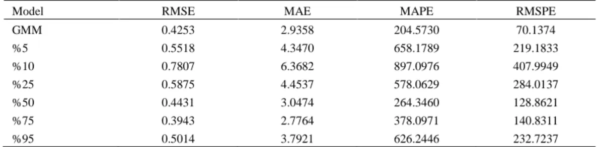
Table 5. Forecast performance statistics
Model RMSE MAE MAPE RMSPE
GMM 0.4253 2.9358 204.5730 70.1374 %5 0.5518 4.3470 658.1789 219.1833 %10 0.7807 6.3682 897.0976 407.9949 %25 0.5875 4.4537 578.0629 284.0137 %50 0.4431 3.0474 264.3460 128.8621 %75 0.3943 2.7764 378.0971 140.8311 %95 0.5014 3.7921 626.2446 232.7237
According to the results in Table 5, the forecast performance of GMM can be evaluated differently for each quantile of the dynamic quantile panel regression model. Considering the Root Mean Squared Error (RMSE) for comparison, we find that the RMSE is 0.4253 for GMM and 0.3943 for the 75th quantile of the dynamic panel quantile model. However, the RMSE is 0.5518 for the 5th quantile. Consequently, the forecast performance of quantile regression changes by quantiles as compared to GMM’s forecast performance.
7. Conclusion
In order to investigate BIST-100 manufacturing industry market in terms of efficiency, 83 companies whose stocks have been traded in BIST-100 during the period of 2000-2014 were considered. The relationship between stock returns and financial ratios (leverage rate, total return on assets, dividend yield, financial beta, market value /book value) were analyzed by using quantile regression for dynamic panel data with fixed effects. There are many articles available in the literature investigating the relationships between stock returns and financial ratios. However since heterogeneous structure of financial variables are not taken into consideration in majority of these studies, that is, the effects of financial ratios on stock returns are assumed same for each parts of conditional distribution of returns, estimators in these models based on Gaussian conditions can be biased. Therefore, panel quantile regression model was used in the investigation of the relationship between stock returns and financial ratios. Since the fixed effect estimator will be biased in case of that the lagged of dependent variable was used as an explanatory variable, quantile regression-instrument variable approach that is suggested by Chernozhukov ve Hansen (2005, 2006, and 2008) was utilized.
According to the estimation results of quantile regression-instrument variable model, stock returns do react differently to the changes in the financial ratios for different parts (5th, 10th, 25th, 50th, 75th, 95th quantiles) of the conditional distribution of returns. Furthermore, the financial ratios’ explanatory power on the change of stock returns varies also for each considered quantile. The quantile regression for dynamic panel model with fixed effects was also estimated without using instrument variable and all of the coefficients of the model were found statistically insignificant.
Consequently, there could be two different conclusions we may draw out of this study. Firstly, stock returns react differently for different parts of the conditional distribution to the changes in financial ratios. Secondly, the existing effects of the financial ratios on the stock returns represent that investors can make future projections about stocks by taking the financial ratios into their consideration and these projections change from high quantiles to low quantiles.
Moreover, BIST-100 manufacturing industry has bear market characteristics for the sample period and it can be said easily that it is not an efficient market. Accordingly since manufacturing industry market is not efficient, the stock returns are predictable.
References
Ahn, S. C., & Schmidt, P. (1995). Efficient estimation of models for dynamic panel data. Journal of Econometrics, 68, 5-27. http://dx.doi.org/10.1016/0304-4076(94)01641-C
Aktaş, M. (2008). A research on financial ratios related to stock returns in the Borsa Istanbul. Istanbul University Journal of the School of Business Administration, 37(2), 137-150.
Anderson, T. W., & Hsiao, C. (1981). Estimation of dynamic models with error components. Journal of the American Statistical Association, 76, 598-606. http://dx.doi.org/10.1080/01621459.1981.10477691
Anderson, T. W., & Hsiao, C. (1982). Formulation and estimation of dynamic models using panel data. Journal of Econometrics, 18, 47-82. http://dx.doi.org/10.1016/0304-4076(82)90095-1
Ang, A., & Bekaert, G. (2007). Stock Return Predictability: Is It There? The Review of Financial Studies, 20, 651-707. http://dx.doi.org/10.1093/rfs/hhl021
Arellano, M., & Bond, S. (1991). Some tests of specification for panel data: Monte Carlo evidence and an application to employment equations. Review of Economic Studies, 58, 277-279. http://dx.doi.org/10.2307/2297968
Artmann, S., Finter, P., & Kempf, A. (2012). Determinants of expected stock returns: Large sample evidence from the German market. Journal of Business Finance and Accounting, 39, 758-784. http://dx.doi.org/10.1111/j.1468-5957.2012.02286.x
Aydemir, O., Ogel, S., & Demirtaş, G. (2012). The Role of Financial Ratios in Determining the Stock Prices. Celal Bayar UniversityJournal of the Faculty of Economics and Administrative Sciences, 19(2), 278-288.
Bali, T. G., Demirtas, K. O., & Tehranian, H. (2008). Aggregate Earnings, Firm-Level Earnings, and Expected Stock Returns. Journal of Financial and Quantitative Analysis, 43(3), 657-684. http://dx.doi.org/10.1017/S0022109000004245
Barber, B. M., & John, D. L. (1997). Firm Size, Book-To-Market Ratio, and Security Returns: A Holdout Sample
of Financial Firms. Journal of Finance, 52(2), 875-883.
http://dx.doi.org/10.1111/j.1540-6261.1997.tb04826.x
Bhandari, L. C. (1988). Debt/Equity Ratio and Expected Common Stock Returns: Empirical Evidence. Journal of Finance, 43(2), 507-528. http://dx.doi.org/10.1111/j.1540-6261.1988.tb03952.x
Blundell, R., & Bond, S. R. (1998). Initial conditions and moment restrictions in dynamic panel data models.
Journal of Econometrics, 87(1), 115-143. http://dx.doi.org/10.1016/S0304-4076(98)00009-8
Bun, M. J., & Carree, M. A. (2005). Bias-corrected estimation in dynamic panel data models. Journal of Business and Economic Statistics, 23(2), 200-210. http://dx.doi.org/10.1198/073500104000000532
Caglayan, E., & Kangalli, S. (2011). Analysis of Binary Panel Data by Static and Dynamic Logit Models: Stock Returns and Macroeconomic Factors. The Empirical Economics Letters, 10(5), 496-501.
Campbell, J. Y., & Shiller, R. J. (1987). Cointegration and tests of present value model. Journal of Political Economy, 95, 1088-1602. http://dx.doi.org/10.1086/261502
Campbell, J. Y., & Yogo, M. (2006). Efficient tests of stock return predictability. Journal of Financial Economics,
81, 27-60. http://dx.doi.org/10.1016/j.jfineco.2005.05.008
Chernozhukov, V., & Hansen, C. (2006). Instrumental quantile regression inference for structural and treatment effects models. Journal of Econometrics, 132(2), 491-525. http://dx.doi.org/10.1016/j.jeconom.2005.02.009 Cohen, R. B., Gompers, P. A., & Vuolteenaho, T. (2002). Who underreacts to cashflow news? Evidence from trading between individuals and institutions. Journal of Financial Economics, 66, 409-462. http://dx.doi.org/10.1016/S0304-405X(02)00229-5
Fairfield, P. M., Whisenant, S., & Yohn, T. L. (2003). Accrued earnings and growth: Implications for future profitability and market mispricing, The Accounting Review, 78(1), 353-371. http://dx.doi.org/10.2308/accr.2003.78.1.353
Fama, E. F., & French, K. R. (2008). Dissecting Anomalies. Journal of Finance, 63(4), 1653-1678. http://dx.doi.org/10.1111/j.1540-6261.2008.01371.x
Fama, E. F., & Kenneth, R. F. (1992). The Cross-Section of Expected Stock Returns. Journal of Finance, 47(2), 427-465. http://dx.doi.org/10.1111/j.1540-6261.1992.tb04398.x
Fama, E. F., & French K. R. (1988). Dividend Yields and Expected Stock Returns. Journal of Financial Economics, 22, pp.3-25. http://dx.doi.org/10.1016/0304-405X(88)90020-7
Franses, P. H., & Dijk, D. (2003). Selecting a Nonlinear Time Series Model using Weighted Tests of Equal Forecast Accuracy. Oxford Bulletin of Economics and Statistics, 65, 727-744. http://dx.doi.org/10.1046/j.0305-9049.2003.00091.x
Galvao, Jr. A. F. (2011). Quantile regression for dynamic panel data with fixed effects. Journal of Econometrics,
164, 142-157. http://dx.doi.org/10.1016/j.jeconom.2011.02.016
Hadri, K., & Kurozumi, E. (2012). A Simple Panel Stationarity Test in the Presence of Serial Correlation and a Common Factor. Economics Letters, 115, 31-34. http://dx.doi.org/10.1016/j.econlet.2011.11.036
Harding, M., & Lamarche, C. (2009). A quantile regression approach for estimating panel data models using instrumental variables. Economics Letters, 104(3), 133-135. http://dx.doi.org/10.1016/j.econlet.2009.04.025 Haugen, R. A., & Baker, N. L. (1996). Commonality in the determinants of expected stock returns. Journal of
Financial Economics, 41(3), 401-439. http://dx.doi.org/10.1016/0304-405X(95)00868-F
Heckman, J. J. (1981). Heterogeneity and State Dependence in Structural Analysis of Discrete Data. Cambridge: MA, MIT Press.
Hjalmarsson, E. (2010). Predicting Global Stock Returns. Journal of Financial and Quantitative Analysis, 45(1), 49-80. http://dx.doi.org/10.1017/S0022109009990469
Hodrick, R. (1992). Dividend Yields and Expected Stock Returns: Alternative Procedure for Inference and Measurement. Review of Financial Studies, 5(3), 357-386. http://dx.doi.org/10.1093/rfs/5.3.351
Jiang, X., & Lee, B. S. (2007). Stock returns, dividend yield, and book-to-market ratio. Journal of Banking & Finance, 31(2), 455-475. http://dx.doi.org/10.1016/j.jbankfin.2006.07.012
Johnson, T. C. (2004). Forecast Dispersion and the Cross Section of Expected Returns. TheJournal of Finance,
59(5), 1957-1978. http://dx.doi.org/10.1111/j.1540-6261.2004.00688.x
Kheradyar, S., Ibrahim, I., & Nor, F. M. (2011). Stock Return Predictability with Financial Ratios. International Journal of Trade,Economics and Finance, 2(5), 391-396. http://dx.doi.org/10.7763/IJTEF.2011.V2.137 Koenker, R. (2004). Quantile regression for longitudinal data. Journal of Multivariate Analysis, 91, 74-89.
http://dx.doi.org/10.1016/j.jmva.2004.05.006
Koenker, R., & Bassett, G. Jr. (1978). Regression Quantiles. Econometrica, 46(1), 33-50. http://dx.doi.org/10.2307/1913643
Korkmaz, Ö ., & Karaca, S. S. (2013). The Factors Affecting Firm Performance: The Case of Turkey. Ege Academic Review, 169-179.
Kothari, S. P., & Shanken, J. (1997). Book-to-Market, Dividend yields, and Expected Market Returns: A time series analysis. Journal of Financial Economics, 44, 169-203. http://dx.doi.org/10.1016/S0304-405X(97)00002-0
Lam, K. S. K. (2002). The Relationship between Size, Book-to-Market Equity Ratio, Earnings-Price Ratio, and Return for the Hong Kong Stock Market. Global Finance Journal, 13, 163-179. http://dx.doi.org/10.1016/S1044-0283(02)00049-2
Lewellen, J. (2004). Predicting Returns with Financial Ratios. Journal of Financial Economics, 74, 209-235. http://dx.doi.org/10.1016/j.jfineco.2002.11.002
Litner, J. (1965). The valuation of Risk Assets and the Selection of Risky Investments in Stock Portfolios and Capital Budgets. The Review of Economics and Statistics, 47(1), 13-37. http://dx.doi.org/10.2307/1924119 Mello, M., & Perrelli, R. (2003). Growth equations: a quantile regression exploration. The Quarterly Review of
Economics and Finance, 43(4), 643-667. http://dx.doi.org/10.1016/S1062-9769(03)00043-7
Modigliani, F., & Miller, M. H. (1958). The Cost of Capital, Corporation Finance, and the Theory of Investment.
The American Economic Review, 48, 261-297.
Mossin, J. (1966). Equilibrium in a Capital Asset Market. Econometrica, 34(4), 768-783. http://dx.doi.org/10.2307/1910098
Nargelecekenler, M. (2011). Stock Prices and Price/Earning Ratio Relationship: A Sectoral Analysis with Panel Data. Business and Economics Research Journal, 2(2), 165-184.
Pesaran, M. H. (2007). A Simple Panel Unit Root Test in the Presence of Cross Section Dependence. Journal of Applied Econometrics, 22(2), 265-312. http://dx.doi.org/10.1002/jae.951
Sharp, W. (1964). Capital Asset Prices: A Theory of Market Equilibrium under Conditions of Risk. The Journal of Finance, 19(3), 425-442. http://dx.doi.org/10.1111/j.1540-6261.1964.tb02865.x
Timmermann, A., & Cenesizoglu, T. (2008). Is the Distribution of Stock Returns Predictable? Working Paper, HEC Montreal and University of California at San Diego.
Vuolteenaho, V. (2000). Understanding the aggregate book-to-market ratio and its implications to current equity-premium expectations. Working paper, Harvard University.
Vuolteenaho, V. (2002). What drives firm-level stock returns? Journal of Finance, 57(1), 233-264. http://dx.doi.org/10.1111/1540-6261.00421
Westerlund, J. (2008). Panel cointegration tests of the Fisher effect. Journal of Applied Econometrics, 23(2), 193-233. http://dx.doi.org/10.1002/jae.967
Note
Note 1. Whether the error terms are distributed normally were investigated by means of Jarque-Bera statistics, skewness and kurtosis. Results showed that error terms did not have normal distribution. Also, it was observed that there are extreme values in the data set through Kernel density functions.
Copyrights
Copyright for this article is retained by the author(s), with first publication rights granted to the journal.
This is an open-access article distributed under the terms and conditions of the Creative Commons Attribution license (http://creativecommons.org/licenses/by/3.0/).