The Cross Section of Expected Returns: Evidence from Implied Beliefs of Active Mutual Funds Managers

(1)

Washington University in St. Louis

Washington University Open Scholarship

Doctor of Business Administration Dissertations

Olin Business School

Spring 4-18-2019

The Cross Section of Expected Returns: Evidence

from Implied Beliefs of Active Mutual Funds

Managers

Jorge Sabat

Washington University in St. Louis

Follow this and additional works at:

https://openscholarship.wustl.edu/dba

Part of the

Business Administration, Management, and Operations Commons

, and the

Portfolio

and Security Analysis Commons

This Dissertation is brought to you for free and open access by the Olin Business School at Washington University Open Scholarship. It has been accepted for inclusion in Doctor of Business Administration Dissertations by an authorized administrator of Washington University Open Scholarship. For more information, please [email protected].

Recommended Citation

Sabat, Jorge, "The Cross Section of Expected Returns: Evidence from Implied Beliefs of Active Mutual Funds Managers" (2019). Doctor of Business Administration Dissertations. 6.

(2)

WASHINGTON UNIVERSITY IN ST. LOUIS

Olin Business School

Dissertation Examination Committee:

Radhakrishnan Gopalan (Chair) Asaf Manela

Deniz Aydin

The Cross Section of Expected Returns:

Evidence from Implied Beliefs of Active Mutual Funds Managers

by Jorge Sabat

A dissertation presented to the Olin Business School in partial fulfillment of the requirements for

the degree of Doctor of Business Administration in Finance

April 2019 Saint Louis, Missouri

(3)

(4)

List of Figures

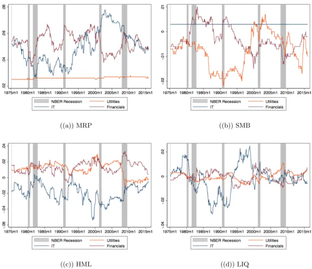
Figure 1 Non-Tradable Factors . . . 30

Figure 2 Contribution to Monthly Expected Return of Sector by Risk Factor of the CAPM model . . . 32

Figure 3 Contribution to Monthly Expected Return of Sector by Risk Factor of the FF3 model . . . 32

Figure 4 Contribution to Monthly Expected Return of Sector by Risk Factor of the FF5 model . . . 33

Figure 5 Contribution to Monthly Expected Return of Sector by Risk Factor of the FF3 MOM LIQ model . . . 34

Figure 6 Contribution to Monthly Expected Return of Sector by Risk Factor of the FF3 MOM model . . . 35

Figure 7 Contribution to Monthly Expected Return of Sector by Risk Factor of the FF3 LIQ model . . . 36

Figure 8 Contribution to Monthly Expected Return of Sector by Risk Factor of the CRR model . . . 37

Figure 9 Mean Conditional Correlation of Sectors Returns by Asset Pricing Model . . . 49

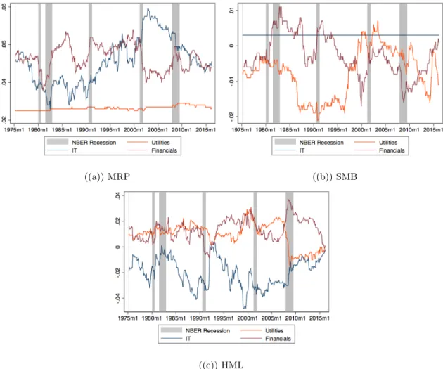
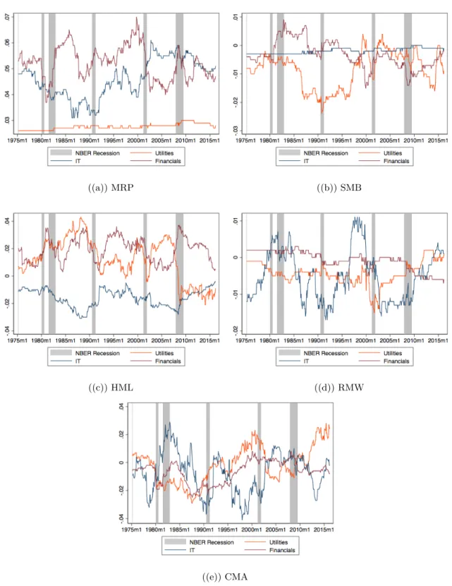
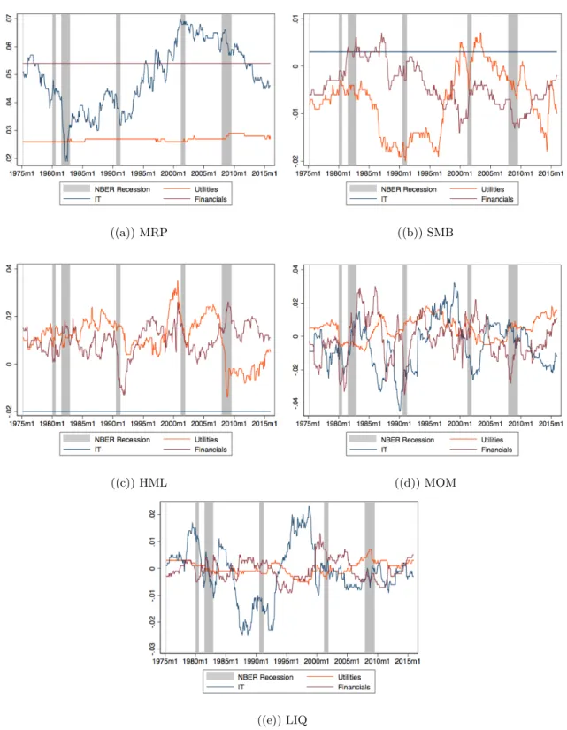
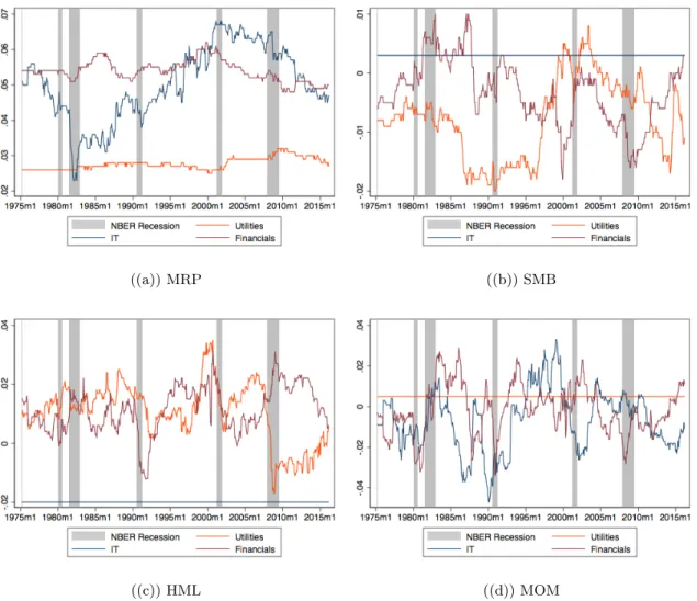
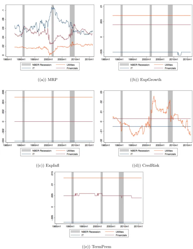
Figure 10 Estimated Implied MRP Premium by Model . . . 55

Figure 11 Estimated Implied SMB Premium by Model . . . 56

Figure 12 Estimated Implied HML Premium by Model . . . 57

Figure 13 Estimated Implied MOM Premium by Model . . . 58

Figure 14 Estimated Implied LIQ Premium by Model . . . 59

Figure 15 Estimated Implied RMW Premium by Model . . . 60

Figure 16 Estimated Implied CMA Premium by Model . . . 61

(7)

Figure 18 Estimated Implied ExpGrowth Premium by Model . . . 63 Figure 19 Estimated Implied TermPrem Premium by Model . . . 64 Figure 20 Estimated Implied CredRisk Premium by Model . . . 65 Figure 21 Cross sectionalR2of Implied Expected Returns by Asset Pricing Model 66 Figure 22 Model versus Empirical Estimation of Market Portfolio’s Sharpe Ratio 67 Figure 23 Structural Error Analysis - CAPM Model . . . 68 Figure 24 Structural Error Analysis - FF3 MOM LIQ Model . . . 69 Figure 25 Structural Error Analysis - CRR Model . . . 70

(8)

List of Tables

Table 1.1 Summary Statistics of Sector Indices Returns . . . 38 Table 1.2 Summary Statistics of Risk Factor time-series . . . 38 Table 1.3 Summary Statistic of Betas of Kalman Filter Estimation by Model

(Panel A) . . . 39 Table 1.4 Summary Statistic of Betas from Kalman Filter Estimation by Sector

and Asset Pricing Model (Panel B) . . . 40 Table 1.5 Summary Statistic of Betas from Kalman Filter Estimation by Sector

and Asset Pricing Model (Panel C) . . . 41 Table 1.6 Summary Statistic of Betas from Kalman Filter Estimation by Sector

and Asset Pricing Model (Panel D) . . . 42 Table 1.7 Standardized Estimates: Contribution of Risk Factors to Sectors

Ex-pected Returns by Asset Pricing Model (Panel A) . . . 43 Table 1.8 Standardized Estimates: Contribution of Risk Factors to Sectors

Ex-pected Returns by Asset Pricing Model (Panel B) . . . 44 Table 1.9 Standardized Estimates: Contribution of Risk Factors to Sectors

Ex-pected Returns by Asset Pricing Model (Panel C) . . . 45 Table 1.10 Standardized Estimates: Contribution of Risk Factors to Sectors

Ex-pected Returns by Asset Pricing Model (Panel D) . . . 46 Table 1.11 Summary Statistics of Historical Mutual Fund Portfolio Weights by

Sector . . . 47 Table 1.12 Summary Statistics of Historical Sector Weights in CRSP Data . . . 47 Table 1.13 Mean Conditional Volatility by Sector and Asset Pricing Model . . . 48 Table 1.14 Mean Conditional Idiosyncratic Volatility by Sector and Asset Pricing

Model . . . 48 Table 1.15 Implied Expected Returns: CAPM . . . 49 Table 1.16 Implied Expected Returns: FF3 . . . 50

(9)

Table 1.17 Implied Expected Returns: FF3 MOM . . . 50

Table 1.18 Implied Expected Returns: FF3 MOM LIQ . . . 50

Table 1.19 Implied Expected Returns: FF5 . . . 51

Table 1.20 Implied Expected Returns: CRR . . . 51

Table 1.21 Example of Expected Returns by Asset Pricing Model at Non-Recession Periods . . . 51

Table 1.22 Example of Expected Returns by Asset Pricing Model at Recession Periods . . . 52

Table 1.23 Factor Premium Estimates by Asset Pricing Model . . . 52

Table 1.24 Summary Statistic of cross sectional R2 by Asset Pricing Model . . . 53

Table 1.25 T-test for Equality of Means of Historical cross sectional R2 _{. . . . .} ₅₃

Table 1.26 Summary Statistic of Model ex-ante Sharpe Ratio and Market Ex-pected Return . . . 54

Table 1.27 Alphas from Time-Series Regressions (Aug-87 to Dec-15) . . . 71

(10)

Acknowledgments

This paper would not have been possible without Pablo Casta˜neda (UAI) guidance and support. I also appreciate the comments of Radhakrishnan Gopalan, Asaf Manela, Deniz Aydin, Xing Huang, Philip Dybvig, and Santiago Trufa.

(11)

INTRODUCTION OF THE DISSERTATION

by Jorge Sabat

A historical analysis of the economic literature shows how empirical research has gained

importance, crowding-out the participation of theoretical research, Hamermesh (2013). This

new trend starts as an effort to settle practical and intellectual debates about economic and

social relationships. These disputed economic relationships, if well understood, can have

real consequences on scientific thinking, politics and business practices.

The main tools that empirical researchers use come from econometrics. Econometrics is the field of economics that study quantitative methods that allow us to unveil different social and economic relationships using empirical data. Specifically, econometrics focuses on formulating tests to evaluate a proposed hypothesis under certain assumptions. Given its “practical usefulness”, econometrics is a central node in the social sciences, gathering researchers from multiple fields that try to test hypothesis that are derived from, more or less, formalized theories. One of the main competitive advantages of econometrics rely on its ability to integrate the best ideas from statistics, and combine it with economic theory to produce its own new method.

One of the potential causes of this shift from theoretical to empirical focus, is the so-called “credibility revolution” (see Angrist and Pischke (2010)). This revolution introduced a new methodological approach when conducting empirical research. This is mainly based on reduced form models, which combined with carefully designed identification strategies, intend to measure the causal effect of an economic variable, as if the researcher would be conducting a quasi experiment. Ideally, this new methodological approach can lead us to reach consensus about the mechanics of the economy, as well as, the effects of certain policies.1 However, even when reduced form quasi experimental methods currently dominate the empirical research scene, there is still a methodological debate with respect to the need (or not) of formalized economic models when conducting empirical research.

1_{One of the main acknowledgements of the “credibility revolution” was its ability to question some well}

(12)

In this thesis, I argue that in different economic debates there is no possible way to escape from a structural econometrics approach. In other words, when analyzing some problems econometricians have to be explicit about the preferences, beliefs and conditional information that determines the behavior of the participants of the social phenomena under study. Specifically, I analyze an old question in the finance literature: Which are the risk factors that drive the stock market movements? A question that after more than 30 years is still open.2 _{In this thesis I will argue that the empirical asset pricing literature has not}

reached consensus, because of the intentional (or unintentional) agnosticism of economic theory. Consequently, I propose a new structural test that microfounds the market equilib-rium, comparing factor models trough the implied beliefs of important market participants, active mutual fund managers. The derivation of the test is based on an heterogenous agent model a la Levy et al. (2006). Where the candidate factor model is the common knowledge that managers use to form their beliefs, and that endogenously determine the market port-folio. I argue that my methodological approach can help us dealing with two important problems that make testing in asset pricing a particularly complex endeavor. First, the joint hypothesis problem raised by Fama (1991). Which imply that any asset pricing test is a joint test of investors preferences, beliefs and the information that determines the market equilibrium. Second, the approximate observational equivalence that asset pricing faces. Which imply that the observed phenomena is consistent with many different theories.3

Finally, the objective of this thesis is to defend a structural approach when conducting empirical research in finance. This imply to not only understand the different microeconomic models that could be relevant to understand a specific economic phenomena, but also to take into account the information asymmetry that exists between the econometrician, and the participants within the analyzed problem.4 Conducting empirical research in this way allow us to evaluate the validity of our hypothesis from different perspectives. First, we can analyze the statistical properties of the estimated parameters, as well as, potential biases in the estimation. Second, we can study the internal validity of the estimated model. Third, we can evaluate the out-of-sample performance of the model.

2_{John Cochrane discuss in detail the problem in his 2011 Presidential Address in the American Economic}

Association.

3

This argument is taken from Mankiw (1989) which makes a similar case for macroeconomics.

4_{Thomas Sargent’s follows this idea of putting the agents of the model at the same level of the}

(13)

In the rest of this thesis I develop my methodological contribution to analyze the classical problem of testing factor models in asset pricing.

(14)

Chapter 1

The Cross Section of Expected Returns:

Evidence from Implied Beliefs of Active Mutual Funds Managers

Introduction

The plethora of asset pricing factors thrown out by the empirical research has increased the need for empirical tests that can identify the model that best explains observed returns. In this paper I use the observed sector holdings of mutual fund managers to back out the factor model that is consistent with their asset allocation. Consistency in my setting is determined by the ability of the systematic factors to best explain the observed risk-return trade-off in the market portfolio.

I focus on active mutual fund managers for the following three reasons. First, despite the growth in passive investment, active mutual funds still constitute the majority of delegated assets under management. They constitute roughly 57% of the assets under management as of March 2017 (EPFR Global). Active funds also account for 95% of the trading volume (Vanguard). Second, a large volume of research highlights that changes in funds asset allocation can provide valuable information. For example, Froot and Teo (2008) show that institutional investors tend to reallocate across size, value/growth and industries. Busse and Tong (2012) show that industry-selection skill drives persistence in relative performance. Kacperczyk et al. (2005) show that investment ability is more evident among managers who hold portfolios concentrated in a few industries. Cremers and Petajisto (2009) show that active share against funds’ benchmark predicts fund performance. Third, if active mutual

(15)

fund managers are closer to the “informed traders” of the asset pricing models that follow the tradition of Kyle (1985), understanding how they take investment decisions can help us to understand the systematic risk factors behind the unobserved “fundamental prices” in Barberis and Shleifer (2003).1

In this paper I follow a structural approach to test asset pricing models as opposed to a reduced form method that is widely used in the empirical asset pricing literature. My main reason is the often argued drawback of the reduced form methods. The reduced form asset pricing tests evaluate factor models based on their ability to eliminate pricing errors, or based on their ability to explain the cross section of expected returns. However, if parameters are non-stationary, there is measurement error in the risk factors, and returns are not normal, there is uncertainty with respect to the power of the tests, in other words, is difficult to asses the ability of a test to correctly reject an incorrect candidate factor model, Harvey and Zhou (1990). Another advantage of not using asset returns to study which systematic factors matter for asset pricing is due to \citet {black1986noise} who argues that returns reflect both information and noise. In such a scenario, Kosak et al. (2017) show that the first principal component that explain expected returns, may not shed light on the actual systematic factors driving asset prices.

The proposed methodology in this paper can be summarized in four steps. First, I construct a panel of active mutual fund industry allocations. Second, I select a set of well-known asset pricing models that include the CAPM, Fama French three and five-factor models, momentum, liquidity and macrofounded risk factors. Third, under the assumption that fund managers use assets’ conditional factor loadings and the conditional variance-covariance matrix of the assets, I reverse the optimal mean-variance portfolio problem that managers solve given an observed asset allocation and a specific candidate asset pricing model. Note that in order to obtain managers’ implied expected returns, I am following Black and Litterman (1991) at fund level.2 Thus, for each candidate asset pricing model I obtain a panel of implied expected returns. Finally, for each candidate asset pricing model, I estimate the implied expected risk premiums that explain the cross section of implied expected returns. This allows me to calculate the implied Sharpe ratio of the market

1_{This is a reasonable conjecture, given that active funds dedicate significant resources to price discovery}

as is shown by French (2008), and they generate alpha before fees, as in Berk and Green (2004).

2_{Black and Litterman (1991) recovers the implied expected returns from the market portfolio, which}

(16)

portfolio for each candidate asset pricing model.

The main novelty of my methodology is that it estimates the implied factor risk premi-ums that are consistent with the asset allocation of active mutual fund managers under a specific factor model. This is in the spirit of learning the state variables that are of interest for investors from their observed asset allocation. Such state variables will determine asset prices if the market equilibrium is described by Cox et al. (1985). However, if the market equilibrium is determined by a model a la Kyle (1985), and if active mutual fund managers can be thought of as the informed investors, studying their portfolio choice is useful to understand prices. Finally, the different candidate asset pricing models are compared based on two criteria. First, the implied mean-variance efficiency of the market portfolio, a direct implication under the derived market equilibrium. In other words, the model comparison is based on the model that maximizes the expected utility of an investor that invest in the market portfolio under the beliefs produced by the asset pricing models, as if only system-atic factors are priced. Second, the ability of an asset pricing model to track a model free measure of the Sharpe ratio of the market portfolio.

The estimated models in this paper have the following economic implications. First, I show that different candidate asset pricing models explain different industry expected returns, or equivalently, imply a different ranking of sector weights in manager’s portfo-lio. We can see that sectors such as Information Technology, Energy and Healthcare have expected returns that vary significantly, in relative terms, depending on the asset pricing model. Second, I show that the cross sectional mean of expected risk premiums across asset pricing models are similar. However, the cross sectional dispersion suggests a significant variation over time. Indeed, a visual inspection of the estimates, suggests that expected risk premiums follow a dynamic that is related to the business cycle. Particularly, the risk premium implied by the models vary significantly before the dot-com bubble and after the Great Recession. Finally, I find that the CAPM model augmented with macrofounded systematic factors is the one that produces the market portfolio with the highest implied Sharpe ratio. At the same time, I find that this model tracks better a model-free estimation of the dynamic of the Sharpe ratio of the market portfolio. The main result presented in this paper is important, given that is consistent with the most natural systematic risk factors considered early by Chen et al. (1986). The most striking fact of my results is that the

(17)

implied Sharpe ratio produced by the CAPM or any of the other models typically used in the empirical asset pricing literature, including Fama French three and five-factor models, are similar in the cross section, as well as, in terms of their dynamic. These results suggest that macroeconomic risks related to economic growth and inflation, credit risk, and term premium, help to explain the risk premium that informed risk averse investors demand for investing.

This paper mainly contributes to the asset pricing, portfolio choice, and macro-finance literature. For example, I illustrate how finding that managers use a more complex model than the CAPM can be consistent with the incipient literature on rational inattention and portfolio choice, Kacperczyk et al. (2016); Abis (2017a); Valchev et al. (2017). As I show, these findings can explain the fees that investor pay for active asset management, a puzzle that has been in the neoclassical finance literature for long time Gruber (1996); Carhart (1997); French (2008). In my interpretation, active managers add value by explaining assets returns using risk factors not captured by the CAPM. In other words, managers earn a premium from the perspective of investors that believe in the CAPM.3 Second, I intend to reconcile the puzzle raised by Barber et al. (2016); Berk and Van Binsbergen (2016), who using mutual fund flows show that investors appear to be using the CAPM to make their investment decisions. A finding that is puzzling, given the well documented failure of the CAPM to explain stock returns. I argue that the apparent inconsistency between the asset pricing model that matters for managers and investors, is consistent with the delegated asset pricing model of Cornell and Roll (2005), which predicts that if investment decisions are delegated, the preferences and beliefs of individuals would be completely superseded by managers’. Third, as Kosak et al. (2017) argue, in order to answer the question of whether asset pricing is “rational”, we might not be able to escape from structural econometric asset pricing models that use specific assumptions about investors beliefs, preferences, and information sets. I argue that this paper can be part of this approach. Finally, my findings

3_{Financial economists have informally highlighted that the value on active asset management is in the}

ability to focus in the relevant risk factors over time. For example, Burmeister et al. (1994) quote: “...an investment manager can control the risk exposure profile of a managed portfolio. Managers with different traditional styles, such as small-capitalization growth managers and large-capitalization value managers, have differing inherent risk exposure profiles. For this reason, a traditional manager’s risk exposure profile is congruent to a particular Arbitrage Pricing Theory style”. Or the conversation presented in Cochrane (2011) between the author and a fund manager: “You don’t have alpha. I can replicate your returns with a value-growth, momentum, currency and term carry, and short-vol strategy.” He said, “Exotic beta” is my alpha. I understand those systematic factors and know how to trade them. You dont.”.

(18)

suggest that macroeconomic factors, such as economic growth and inflation expectations, credit risk spreads, and term premiums, carry important additional information for asset pricing, something that even when is intuitive when we read Chen et al. (1986), it has been elusive to the empirical asset pricing literature.

The paper proceeds as follows: In the second section, I review the literature. The third section explains the structural model and the connections with the empirical estimates. The fourth section describes the dataset and presents summary statistics. The fifth section presents the results. The final section concludes.

Literature

This paper is related to four strands of the finance literature.

The mutual fund literature. First, the literature on performance measurement, and the value of active versus passive investing. Fama and French (2010), have revisited a perfor-mance analysis of mutual funds, showing that only a small proportion of funds beat the market. Sharpe (1992) showed that a limited number of major market indices are required to successfully replicate the performance of an extensive universe of U.S. mutual funds. On the contrary, others studies defend the role of active mutual funds. For example, Avramov and Wermers (2006) state that active management adds significant value, showing that industries are important in locating outperforming mutual funds. Similarly, Kacperczyk et al. (2014) show that mutual funds stock picking or market timing ability fluctuates with the state of the economy. Indeed Kacperczyk et al. (2016) suggest that skill can be linked to attention allocation. Second, the literature on delegated asset management, and the role of benchmarking, pay-for-performance, and investment constraints. Almazan et al. (2004) show empirical evidence with respect to how investment constraints arise endogenously in mutual funds management. Dybvig and Ross (1985a); Admati and Ross (1985) show that under information asymmetry the client-fund manager relation is distorted. A result that is consistent with investor disagreement in incomplete markets, Cochrane and Saa-Requejo (2000a), and the idea that performance evaluation should be defined in a client-specific fashion as in Sharpe (1982). Third, the empirical literature on mutual fund holdings. Elton et al. (2011) test four well known hypothesis in the mutual funds’ literature, momentum

(19)

trading, tax-motivated trading, window dressing, and tournament behavior. They pro-vide epro-vidence against momentum strategies, while supporting a tax selling motive, window dressing effect at annual frequency, and risk-shifting. Froot and Teo (2008) find strong evidence of mutual funds reallocation across size, value/growth, and industry/sector port-folios. Busse and Tong (2012) find that the “industry selection” component of mutual funds represents roughly half of portfolios’ risk adjusted returns. Kacperczyk et al. (2005) find that industry concentration of mutual funds, determined by some information advantage, is positively correlated with performance. Cremers and Petajisto (2009) find that funds with higher active share, which represents the share of portfolio holdings that differ from the benchmark index holdings, exhibit strong performance persistence. Shumway et al. (2009); Yuan (2007) extract fund manager beliefs on expected stock returns using hold-ings data. They document interesting facts about mutual funds managers’ priors, such as: risk adjustment in portfolio choice decisions; lower correlation of risk-return trade-off in the “small caps” family; less disagreements among large stocks; lack of forecasting abilities. Finally, the normative literature on portfolio choice. Markowitz (1952) pioneered the mean-variance portfolio choice theory. More recently, Grinold (1999), Litterman et al. (2004), and Meucci (2009), have analyzed variations of the mean-variance optimizer problem including views with respect risk and return of investable assets. Avramov and Zhou (2010) review the Bayesian approach in portfolio management, a framework that account for managers’ priors on risk, returns and asset pricing theories.

The empirical asset pricing literature. This literature has mainly focus on identifying models with no asset pricing errors (α) in time-series regressions, Gibbons et al. (1989), or in explaining the cross section of expected returns, Fama and MacBeth (1973). Backed up by these methods, or variations of them, the number of factors went up from 1, aggregated wealth (CAPM) or consumption (CCAPM), to at least 316 factors.4 In an effort to ad-dress the factor zoo, new methodologies have been being proposed. For example, Harvey et al. (2016) proposed stricter statistical rules for the t-statistic of the traditional Fama and MacBeth (1973) two-stage test. Harvey (2017) proposes a minimum Bayes factor to deal with p-hacking. Feng et al. (2017) apply dimension-reduction techniques (double-selection LASSO) to run a Fama-Macbeth regression with 99 factors. Harvey and Liu (2016) and Fama and French (2016) modify the traditional multiple hypothesis test of Gibbons et al.

(20)

(1989). Kan et al. (2013) derive the asymptotic distribution of the cross sectionalR2on ex-pected returns to discriminate asset pricing models. Following a different approach, Barber et al. (2016); Berk and Van Binsbergen (2016) propose a model comparison based on their ability to relate performance measurement and mutual fund flows to understand which factors investors care about. Interestingly, they find that the CAPM is the best model. Nevertheless, this finding raises a puzzle, as is well documented that the CAPM is rejected by traditional tests. On the other hand, Ghosh et al. (2016) proposes a statistical method to understand the missing information in the stochastic discount factor derived under the CCAM. This gives economic support to the Fama-French factors. Finally, Kosak et al. (2017) show that under certain assumptions, reduced-form factor models and characteristic based asset pricing, Daniel and Titman (1997), are not able to differentiate asset pricing theories. Consequently, they call for the development and testing of structural asset pric-ing models with specific assumptions about investors beliefs and preferences that deliver predictions with the discount discount factor that being test.

This paper is also related to an incipient structural econometric literature that analyzes portfolio choice problems. Koijen and Yogo (2015) estimate a model with investor demand to illustrate how their model can be used to understand the role of institutions in asset market movements, volatility, and predictability. Koijen (2014) proposes a structural model that disentangle ability, incentives, and risk preferences of mutual fund managers, providing empirical evidence supporting the model’s implications for the asymmetric flow-performance relationship. Casta˜neda and Devoto (2016) estimate a dynamic portfolio choice model for the case of Chilean pension funds, finding that pension fund mangers are heavily motivated by relative performance. Branikas et al. (2017) propose and estimate a location choice model, typically used in urban economics, to analyze stock local bias and the performance of local stock picks.

Finally, this paper intends to shed light on the relationship between macroeconomics and asset pricing. The macro finance literature has taken different approaches. First, a more structural analysis started with the equity risk premium puzzle of Mehra and Prescott (1985). The authors show that is difficult to reconcile the observed risk and return of the stock market with a reasonable calibrated Lucas (1978)-like model. Similarly, Breeden et al. (1989) rejects the Consumption CAPM. These papers motivated the study of new

(21)

preferences, Benartzi and Thaler (1995), the inclusion of catastrophic risk in the stock market, Barro (2006), and the use heterogeneous agents models, Mankiw and Zeldes (1991). On the other hand, a reduced form approach have found weak responses of stock prices to macroeconomic news, Chen et al. (1986); Fama (1990); Schwert (1990); Campbell (1996). Nevertheless, other authors have argued that the failure of these tests could be more related with the availability of real-time macroeconomic indicators, Christoffersen et al. (2002); Savov (2011), or other measurement problems related with time horizons of returns, Parker and Julliard (2005).

Model

The model economy is a static finance economy. It is populated by a finite number of fund managers (I). The asset market is composed by a risk-free asset that yieldsrf, and a finite number (L) of risky assets that are in positive net supply. The returns of the risky assets obey a linear K-factor structure as in Wei (1988).5

Thus, the excess of return of asset is given by:

rl´rf “β1,lf1`β2,lf2`...`βK,lfK`l (1.1)

where fk is a realization of one of the K-systematic risk factors, and βk,l is the factor loading of asset l associated with risk k. The systematic factors have expected values contained in the vectorµf and a variance-covariance matrix Σf. In addition, assets values face idiosyncratic shocks (l) that are zero in expectation and have a variance-covariance matrix equal to Σ.

An additional feature of this economy are the heterogeneous beliefs of managers that explain why they hold different portfolios. Specifically, I follow P´astor and Stambaugh (2000), who analyze the investment process of asset managers that decide their asset allo-cation combining an asset pricing model and their own specific views.6

5_{This is a generalization of Ross’s Asset Pricing Theory (APT) or Connor’s competitive-equilibrium}

version of the APT. Such that, the Capital Asset Pricing Model (CAPM) can be seen as a special case.

6

The idea is to capture disagreement about the mispricing across assets’ prices. We can think about this case from Black and Litterman (1991) point of view, where mispricing emerges from investors’ disagreement with the prediction of an asset pricing model. In this model mispricing is exogenously parameterized as

(22)

Therefore, by assumption, fund managers have subjective belief about assets’ returns, while they agree on the assets risk structure.7

Mathematically, managers’ belief structure can be denoted by , such that expected re-turns and variance covariance-matrix are given by:

Eirrs “µi“rf1`αi`βErfs

Σ“βΣfβ`Σ

(1.2)

whereαiis a Lx1 vector that contains the mispricing of the L assets from the perspective of investori;β is an NxK matrix that containts the factor loadings of the assets with respect to each of the systematic factors in the economy; Erfs is a Kx1 vector that contains the expected value of K-factors; Σf is the variance-covariance matrix of the factors; Σ is the variance-covariance matrix of the idiosyncratic risks.8

Managers investment decisions consist in allocating their assets under management (ωj) accordingly with its mean-variance preferences and their own beliefs.910

The portfolio choice model is characterized by managers risk aversion (), and their be-liefs (), such that they maximize their expected utility as follows:

max wi w_i|µi´ 1 2γw | iΣwi subject to L ÿ l“1 wl “1 (1.3) w_i˚“ 1 γΣ ´1 pµi´rf1q (1.4) wherew˚

i is a Lx1 vector that contains the optimal portfolio allocation of manageriin

in Levy et al. (2006). Following Levy et al. (2006), the economic rationale behind this argument is to capture the idea that heterogeneity of beliefs may be a result of heterogeneous private information, partial informativeness of prices, differential interpretation of the same information, or overconfidence investors’ priors.

7

This assumption is reasonable in a Merton (1980a) world, where expected returns are more difficult to estimate than variances and covariances.

8

Decomposing managers’ beliefs in a systematic and an idiosyncratic component is in line with the micro-and macroforecasting behavior in the equilibrium model of market timing developed by Merton (1981).

9

Mean-variance preferences are consistent with constant absolute risk aversion preferences, therefore, the size of assets under management (ωj) do not affect portfolio choice decisions. Total financial capital in this

economy is normalized to 1.

10

Mean-variance preferences can be justified from empirical evidence in the neuroscience literature, Preuschoff et al. (2006)

(23)

the assets of this economy.

Given the market structure described above, the financial market equilibrium is given by:

I ÿ i“1 w˚ iωi“ p¨q řL i“1pqi I ÿ i“1 1 γΣ ´1´_µ i´rf1 ¯ ωi“ p¨q řL i“1pqi 1 γΣ ´1´_α `βErfs ¯ “ _ř_Lp¨q i“1pqi “wˆ (1.5)

where řL_i_“₁piqi and ˆw are the total market capitalization, which is equal to the sum product between asset prices (p) and the supply of assets (q), and the market weights of the assets, respectively. As we can see, the left hand side of Equation (1.5) is a well-known result in the heterogeneous belief literature. Market weights ( ˆw) are equivalent to the optimal portfolio choice of a representative agent with consensus expected returns: expectations derived from the asset pricing model (βErfs) plus a weighted average of managers’ specific views (α). The Lx1 vector α contains the consensus mispricing of assets in the economy (αl“

řI

i“1αl,iωi).11

Lemma 1. The described market equilibrium can be classified as:

1. Efficient, when rational expectation holds at the aggregated level, or equivalently, when the sum of the squared pricing errors is equal to zero:

α|α“0

2. Biased, when there is an over or under estimation of the expected returns of the assets from the representative agent perspective:

α|α‰0

Proof. Given the factor structure of stock returns in Equation (1.1), expected returns and

11

(24)

the variance-covariance matrix are equal to:

Errs “µ“rf1`βErfs

Σ“βΣfβ`Σ

As we can see, when:

I

ÿ

i“1

αl,iωi“0,@l“1, ..., L ùñ α|α“0

Rational expectations hold in this economy, as the aggregated beliefs that determine the market equilibrium coincide exactly with the expectations derived from the asset pricing model that determines assets returns. Equivalently, we can see that the market portfolio is mean-variance efficient, as:

ˆ wt“ 1 γΣ ´1´_βE rfs ¯

On the other hand, when:

I

ÿ

i“1

αl,iωi‰0 ùñ α|α‰0,@l“1, ..., L

There is an excess (lack) of demand on assetlif:

I ÿ i“1 αl,iωią păq0 ùñ 1 γσ ˚ l ´ αl`βlErfs ¯ ą păq1 γσ ˚ l ´ βlErfs ¯ whereσ˚

l is thelrow of the inverse of the variance-variance matrix (Σ); αl is the consensus mispricing of assetl;βl is the l row of the loadings matrix (β).

An implicit assumption of the described market equilibrium is that, abstracting from systematic mispricing (α“0), the market risk premium ( ˆwµ´rf “wˆ|βErfs) is internally consistent with investors preferences and the information structure in the model economy. Particularly, is taken as given that the risk premium is consistent with the portfolio al-location of a mean-variance investor with risk aversion equal to γ. In such a way that the financial market, which is in positive net supply ( ˆwą0q) clears, given the systematic ( ˆw|Σfwˆ) and idiosyncratic ( ˆw|Σwˆ) risk exposure of the market portfolio. In order to

(25)

well establish the market equilibrium, additional conditions have be imposed. Combining the market equilibrium analysis of with the specific asset pricing structure in the analyzed economy, equilibrium expected returns in this economy have to satisfy that:

µ´rf1“γ ´ Σf `Σ ¯ ˆ w«βErfs (1.6)

As we can see, if the variance-covariance matrix of assets returns is positive definite, and assets are in positive net supply, assets have to carry a positive risk premium. This premium is positively related to investors risk aversion, and their risk exposure. Finally, interpreting the factor loading matrix (β) as a multivariate measure of the systematic risk exposure of the assets, the expected value of the risk factors (Erfs) can be interpreted as risk premiums (or compensations) for bearing multiple risks, given an absolute risk aversion level (γ). On the other hand, the market price of risk in this economy, can be calculated by the Sharpe Ratio (SR) of the market portfolio, as follows:

SRpwˆq “ b

pµ´rf1q|Σ´1pµ´rf1q

Econometric Problem

In this section I describe my microeconometric methodology to test which asset pricing model is consistent with the financial market equilibrium described above. I follow a decision theory approach in econometrics, in the spirit of McFadden (1986).12 Accordingly, I start with a decomposition of the asset allocation problem (decision making process) of an active mutual fund manager (decision maker) into the following components:

1. Choice set:

(a) Top-down allocation in US industries.

2. Beliefs:

(a) Asset pricing model (M);

12_{McFadden (1986) focus on consumer research from a marketing science point of view. Thus, the proposed}

methodology in this paper can be seen as a financial economics adaptation of MaFadden’s methodological approach.

(26)

(b) Mangers specific views (αi,t).

3. Latent variables:

(a) Factor loadings (βM,t);

(b) Variance-covariance of systematic risks (ΣM,f,t);

(c) Variance-covariance of idiosyncratic risks (ΣM,,t).

4. Observable variables:

(a) Historical returns of the investable assets;

(b) Evolution of the risk factors.

5. Preferences:

(a) Mean-variance preferences with risk aversion (γ).

6. Decision protocol:

(a) Expected utility maximization conditioned on beliefs, preferences and latent vari-ables.

7. Behavioral output:

(a) Asset allocation decision (w˚

i,t).

Consistently with the structure of the asset allocation decision process described above, a microfounded test of the financial market equilibrium can be formulated from: i) Proposing a set of candidate asset pricing models to be tested; ii) A method for inferring the latent variables under different asset pricing models; iii) An estimation procedure that connects candidate asset pricing models with the data of managers asset allocation decisions; iv) Quantifiable criteria to discriminate among the asset pricing models that are being tested. In the rest of this section, I expand on these aspects of the econometric test.

Candidate Asset Pricing Models

I focus on a set of seven reduced form factor models that are important in the empirical asset pricing literature, covering a broad class of theories that intend to explain asset prices:

(27)

i) CAPM; ii) Fama and French Three Factor Model, Fama and French (1993), FF3; iii) Fama and French Five Factor Model, Fama and French (2015); iv) Fama and French Three Factor Model with momentum, Carhart (1997), FF3 MOM; v) Fama and French Three Factor Model with P´astor and Stambaugh (2003a) liquidity factor, FF3 LIQ; vi) Fama and French Three Factor Model with momentum and liquidity factors, FF3 MOM LIQ; vii) An adaptation of the macrofounded model of Chen et al. (1986), CRR. The risk factors included in the different evaluated models proxy for the following systematic factors that determine asset prices:

1. The market factor (MRP) of the Capital Asset Pricing Model (CAPM) is a natural benchmark, as it proxy for the aggregated wealth in the economy.

2. The size (SMB) and value (HML) factors of Fama and French (1993). Vassalou (2003) suggests that SMB and HML factors contain information related to future GDP growth.

3. The investment (CMA) and profitability (RMW) factors of Fama and French (2015). These factors are important in production based asset pricing models a la Hou et al. (2015).

4. The liquidity factor (LIQ) of P´astor and Stambaugh (2003a). Liquidity as a system-atic factor in general equilibrium asset pricing models has been mainly related with solvency constraints, Chien and Lustig (2009), corporations’ desire to hoard liquidity, Holmstr¨om and Tirole (2001), and flight to liquidity, Acharya and Pedersen (2005).

5. The momentum factor (MOM) of Carhart (1997). Momentum has been mainly related with slow information diffusion, Hong and Stein (1999), or sentiment, Barberis et al. (1998).

6. The macrofounded risk factors proposed by Chen et al. (1986). A growth expecta-tion factor (ExpGrowth), an inflaexpecta-tion expectaexpecta-tion factor (ExpInfl), a term premium factor (TermPrem), and a credit risk factor (CredRisk). Chen et al. (1986) rationale behind the inclusion of these factors is mainly related with analyst valuation process, cash flows forecasting (economic growth and inflation expectations) and discount rate determination (market risk, credit risk and term premium).

(28)

Latent Variables Inference

In this subsection I explain how factor loadings, and the variance-covariance of systematic and idiosyncratic risks, key latent variables in the asset allocation process, are inferred from the econometrician perspective. I assume that fund managers learn about the factor loadings, and the variance-covariance of systematic and idiosyncratic risks, using statistical models that exploit available information about returns and the risk factors. From the econometrician point of view, I model this learning process using the following conditional time-series models.

First, the conditional estimation of factor loadings is performed via the Kalman filter, as in Adrian and Franzoni (2009). The statistical model consist in a linear regression of historical returns of the assets on the risk factors, where factor loadings (β), as well as, the model misspring parameter (λ) follow AR(1) process.

rj,t “cj,M,t`βj,M,tft,M `uj,t (1.7)

βj,M,t“ω1`βj,M,t´1`vj,t (1.8)

cj,M,t“ω2`λj,M,t´1`j,t (1.9)

whererj,t is the return of asset j,cj,M,t is asset j mispricing under modelM at timet, βj,M,t is a vector of factor loadings associated with model M at time t, ft,M describes the evolution of factors under model M at time t, and u, v and are iid normally distributed error terms.

Consistently with the conditional factor loading estimations, idiosyncratic returns by asset (j), model (M), are calculated as follows:

uj,t,M “rt´βM,tft,M (1.10)

Then, the conditional variance-covariance matrix of idiosyncratic returns is estimated with a Multivariate ARCH(1) without conditioning variables in the mean, following Engle (2002) econometric implementation.

(29)

On the other hand, the conditional variance-covariance matrix of factors Σt,M is esti-mated using a Multivariate GARCH(1,1) without conditioning variables in the mean, as in Bauwens et al. (2006)).

Eliciting Asset Pricing Beliefs from Mutual Funds Asset Allocation

In this section I propose an econometric method to elicit asset pricing beliefs from ob-served funds asset allocation. First, given a candidate asset pricing modelM, the following transformation of the cross section of portfolio weights for every asset manager (i) at each moment of time (t) can be performed:

µj,M,t“rf,t1`ΣM,twj,t (1.11)

This transformation is a direct consequence of reverse engineering the solution of mangers’ asset allocation problem. Given the conditional variance-covariance matrix of assets (ΣM,t), the observed risk free rate, a normalized risk aversion level (γ) fixed to 1, and manger’s j

observed asset allocation decisions (wj,t).13

Second, given the assumption of implied expected returns being formed by a systematic component plus managers’ specific views. The following OLS regression recovers a projec-tion of the factors onto the cross-secprojec-tion of implied expected returns, under a candidate asset pricing model (M):

µt,M “βM,tfr_M,t`α_t,M (1.12)

whereµt,M is a stacked vector of implied expected returns of managers, calculated under an asset pricing modelM;fr_M,tis a vector that contains estimated consensus risk premiums

associated to risk factors embedded in a specific asset pricing model M; βM,t is a matrix of conditional factor loadings;αt,M is a stacked vector that contains the “structural errors”

13_{In order to be precise, from Equation (1.6), we can see that the risk aversion parameter is not identified.}

Thus, under my specification, we are recovering a combination of risk preferences and beliefs. Nevertheless, I argue that this can be seen as an analogy of Chetty (2009) sufficient statistics, given that they main idea of the proposed test is to learn about the marginal utility of the representative agent, as is explained in my macro-finance interpretation of the test in the Appendix.

(30)

of managers preferences with respect to specific assets.14 The OLS estimation implicitly imposes the Efficient condition (Erαt,M “0s) of Lemma 1, in other words, the estimated implied risk premiums will be such that deviations from the candidate asset pricing model cancel out. As we can see, the proposed test is a microfounded version of the two-pass cross sectional regression of Fama and MacBeth (1973), such that the dependent variable are implied expected returns instead of realized returns, that allow us to estimate implied expected risk premiums for different candidate asset pricing models.

Horse Race of Factor Models

After estimating a set of candidate factor models, the question is, how to evaluate the finan-cial economic validity of a candidate asset pricing model? As has been noted by Jagannathan and Wang (1998); Kan and Zhang (1999); Lewellen et al. (2010), model comparisons based on the cross-sectional goodness of fit (e.g. the R2s of regression (1.12) of a specific candi-date model is problematic if “useless” factors are included, or due to omitted-variable bias.15 While my estimates suffer from the same potential biases of traditional cross-sectional re-gressions that use returns, I argue that in my setting there is a clear reason of why a higher cross-sectionalR2 is not indicative of the probability of a model being the true asset pricing model that determines the market equilibrium. In my framework, a higher R2 is indica-tive of a higher degree of explanatory power of the cross-section of managers investment decisions. However, explaining managers asset allocation better is not necessarily related with understanding the factor model behind the market equilibrium of Equation (1.5) if an “idiosincratic factor” is correlated with (αi). Intuitively, we can think about a risk factor (e.g. momentum or liquidity) that is indicative of disagreement with respect to the value of some assets. Disagreement manifest in managers holding positions (overweighting or underweighting assets) that deviate from the optimal portfolio that is consistent with strict a belief on the asset pricing model, however, even in this case the market equilibrium can be still determined (more or less) by the asset pricing model. In conclusion, I argue that the R2 is problematic as an asset pricing criteria, as it does not allow us to differentiate

14

The concept of structural error comes from Rust (1987a), and is defined by an unobservable (for the econometrician) component of preferences that explain why agents make different choices given the same observables.

15_{Sala-i Martin (1997) discusses a similar problem in his study of the causal drivers of economic growth}

(31)

between systematic versus idiosyncratic risks, both important determinants of investment decisions, but not necessarily of equilibrium prices. Consequently, I propose the following two criteria to compare candidate asset pricing models in my setting:

1. The maximum implied Sharpe Ratio of the market portfolio: The idea of comparing models using the Sharpe ratio is behind the classical test in asset pricing of Gibbons et al. (1989). Importantly, Gibbons et al. (1989) show that testing for mispricing, measured from the constants ( ˆα) of time-series factor regressions, is related with the maximum Sharpe ratio attainable by the test assets (SR˚_{), trough the following}

relation:

ˆ

α|Σˆαˆ“SR˚2´SRM2 (1.13)

where SRM is the Sharpe ratio under a factor model M, and ˆΣ is the estimated variance-covariance matrix of idiosyncratic returns. As we can see, a model that can explain a lower mispricing is equivalent to a model that can generate a higher Sharpe ratio. In Gibbons et al. (1989) the argument behind explaining a lower mispricing is directly related with the idea of no arbitrage opportunities, which is similar to my ex-ante Efficiency condition in Lemma 1. Nevertheless, I argue that in my framework, the discrimination of asset pricing models can be more naturally related with the model that maximize the expected utility of an investor with no assets specific views. Under my assumed preferences, and abstracting from managers private information, this criteria is equivalent to searching for the model that produces a portfolio with the highest Sharpe ratio.16 The procedure to estimate the implied Sharpe ratio of the aggregated market portfolio is the following. First, I estimate the expected return of the aggregated stock market from the perspective of the representative investor, abstracting from biases (α) or as if only systematic risks are priced:

ErRst,M “wˆt|βM,tfr_M,t (1.14)

where ErRst,M is the expected return of the aggregated market at time t under the estimated asset pricing model M; ˆw is a vector that contains the observed market

16

A result that is not inconsistent with the possibility that a skilled manager enhanced the performance of their portfolio utilizing valuable private information, as in Treynor and Black (1973).

(32)

sector weights at time t. Second, I estimate the volatility of the aggregated market as: σrRst,M “ b ˆ wt|ΣM,twˆt (1.15)

The ex-ante Sharpe ratio under modelM is calculated as:

SRt,M “

ErRst,M ´rf,t σrRst,M

(1.16)

Finally, the statistical evaluation of the candidate asset pricing model is trough a simple mean test of the Sharpe ratio time-series by model. Specifically, I test if there is a model that can produce a statistically higher Sharpe ratio then the rest.

2. The second quantifiable criteria that I propose to compare the estimated asset pric-ing models is directly from their ability to explain the Sharpe ratio of the market portfolio. I specifically focus on a model-free measure of the market portfolio Sharpe ratio constructed using historical returns of the market portfolio only. The model-free estimation is constructed combining the following estimates:

(a) The dynamic of the excess of return of the market portfolio is estimated from the trend component of observed monthly excess returns of the market portfolio (ErRst,τ) obtained via the Hodrick-Prescott filter.

(b) The dynamic of the volatility of the market portfolio is estimated from the con-ditional volatility of a fitted GARCH(1,1) process (σrRs˚t).

Such that, the model-free ex-ante Sharpe ratio is constructed as follows:

SRt,τ “

ErRst,τ

σrRs˚_t (1.17)

Finally, the statistical test consist in rejecting if the mean of the estimated Sharpe ratio under modelM is equal to the model-free estimation.

Data and Summary Statistics

Data used in this paper come from a sample of U.S. equity active mutual funds constructed following Koijen (2014) criteria. Specifically, I use Thomson CDA S12 Mutual Fund

(33)

Hold-ings Database, linking it with CRSP Mutual Fund Database using MFLINKS, following Wermers (2000). This allows me to construct a panel database that contains holdings at quarterly/semi-annual frequency, and monthly returns, as well as, other fund level informa-tion, such as: portfolio manger identificainforma-tion, date at which the manager joined the fund, and fees.

In order to reduce the dimensionality of the data, and giving the technical advantages of using portfolio-level returns instead of securities’ in empirical asset pricing tests. I aggregate the assets’ holding data at sector level following the equivalency between SIC codes and GICS sectors proposed by Bhojraj et al. (2003).17 18

As has been mentioned before, the reduced form asset pricing models evaluated in this study are the following: i) CAPM; ii) Fama and French Three Factor Model (FF3); iii) Fama–French five–factor model (FF5); iv) Fama and French Three Factor Model with momentum (FF3 MOM), Carhart (1997); v) Fama and French Three Factor Model with P´astor and Stambaugh (2003a) liquidity factor (FF3 LIQ); vi) Fama and French Three Factor Model with momentum and liquidity factors (FF3 MOM LIQ); vii) An adaptation of the macrofounded model of Chen et al. (1986) (CRR). The construction of the factor mimicking portfolio returns and nontradable factor variables is explained below.19

• The market factor (MRP) of the CAPM is constructed as the excess return on the market value-weight return of all CRSP firms incorporated in the US, with respect to the one-month Treasury bill rate.

• The size (SMB) and value (HML) factors of Fama and French (1993). SMB is con-structed as the average return on the three small portfolios minus the average return on the three big portfolios. HML is constructed as the average return on the two value

17

I use the 10 Global Industry Classification Standard (GICS) sectors, a classification widely used by prac-titioners: Energy, Materials, Industrials, Consumer Discretionary, Consumer Staples, Healthcare, Financials, Information Technology, Telecommunication Services, and Utilities.

18

I evaluate the quality of the mapping based on sectors comparing the returns of the sector mapped portfolio to their actual return. The mapped portfolio returns overestimate mutual fund gross returns by 16 basis points monthly on average, which is close to the average 2% annual fees. While the contemporaneous correlation is 0.893.

19

The data used for the observed risk free rate, Fama and French three-factor model, momentum factor of the Carhart four-factor model, operating profitability and investment factors of the Fama and French five-factor model are all obtained from Kenneth French website in a monthly frequency for the period 1964-2016. The liquidity factor is obtained from Lubos Pastors website in a monthly frequency for the period 1962-2016.

(34)

portfolios minus the average return on the two growth portfolios.

• The profitability (RMW) and investment (CMA) factors of Fama and French (2015). RMW is constructed as the average return on a robust operating profitability portfolio minus a weak profitability portfolio. CMA is constructed as the average return on a conservative investment portfolio versus an aggressive investment portfolio.

• The liquidity factor (LIQ) of P´astor and Stambaugh (2003a). LIQ is constructed as the average return of a portfolio of low liquidity, measured by a stronger volume-related return reversals, minus high liquidity.

• The momentum factor (MOM) of Carhart (1997). MOM is constructed as the average return on the two high prior return portfolios minus the average return on the two low prior return portfolios.

• Macroeconomic factors of Chen et al. (1986). A growth expectation factor (Exp-Growth) is constructed using the first principal component of the University of Michi-gan Consumer Sentiment Index and the Philadelphia Fed Business Outlook Survey Diffusion Index of General Conditions for the period 1980-2016, which are the activ-ity variables that capture more attention by Bloomberg Terminal users. Following the same criteria of Bloomberg attention, the inflation expectation factor (ExpInfl) is measured by the Conference Board Consumer Confidence Inflation Rate Expectation 12m. The term premium factor (TermPrem) is constructed as the excess of return of the Barclays U.S. Treasury index and a 3-month T-Bills portfolio. The credit factor (CredRisk) is constructed as the excess of return of the BofA Merrill Lynch US Cash Pay High Yield index and Barclays U.S. Corporate Investment Grade index.20

In Table 1.1, summary statistics of the historical returns of Datastream sector bench-marks is presented. The sector with the highest (lowest) return during the analyzed period is Consumer Staples (Telecom). In term of risk, the sector with the highest (lowest) volatility is IT (Utilities).

20

In the Appendix, an exploratory data analysis for the constructed non-tradable factors, economic growth expectations and inflation, is documented. Importantly, I show that I can reject non-stationarity in both cases.

(35)

In Table 1.2, summary statistics of the historical evolution of the tradable and non-tradable factors are presented. The non-non-tradable factors are measured in a different scale, as these are not based on mimicking portfolios but are based on the leading indicators described above.

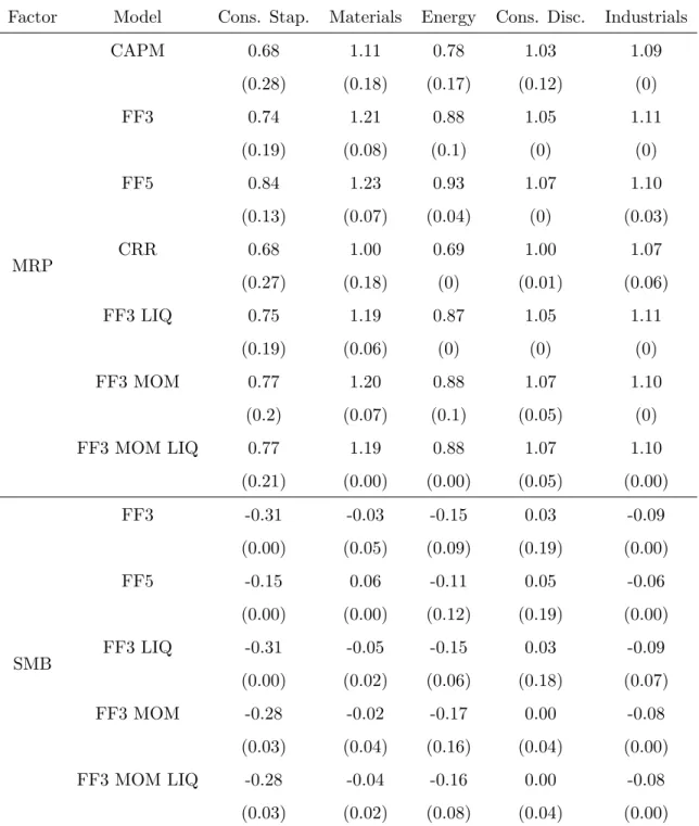
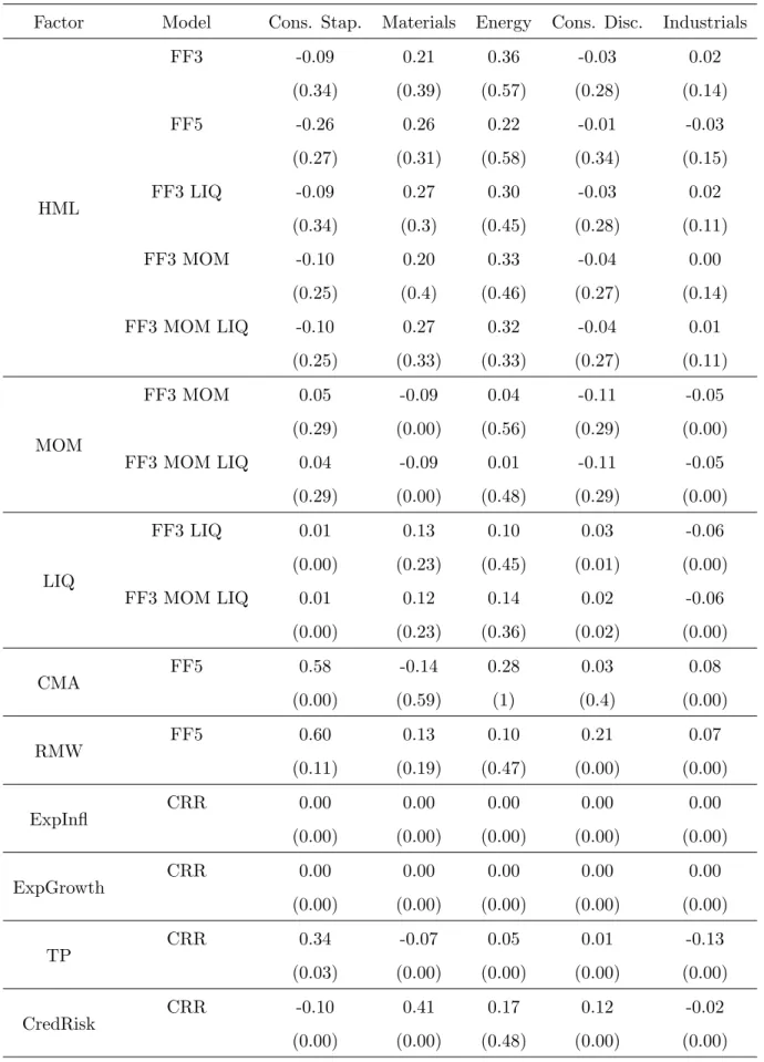
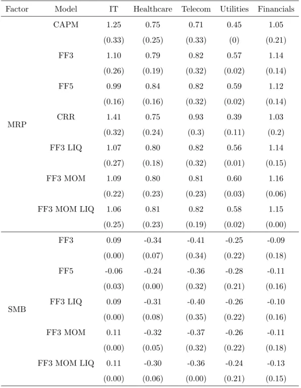
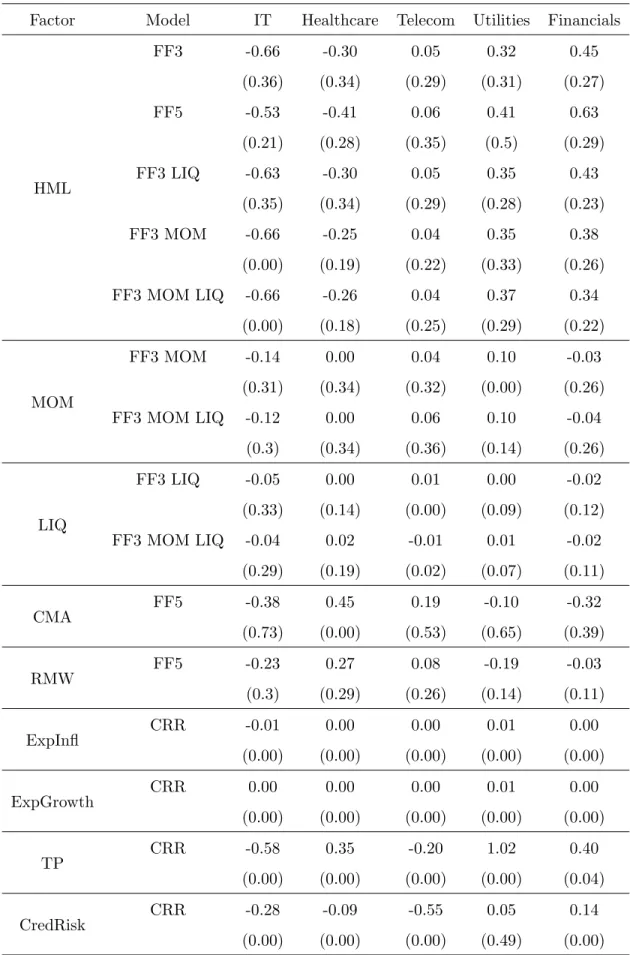
In Table 1.3-1.6, summary statistics of the conditional factor loadings obtained from the proposed Kalman Filter estimation by sectors and asset pricing models. As we can see, on average, betas associated to the same risk factor and sector across models are relatively similar. On the other hand, we can see that conditional betas of some sectors are significantly more volatile than others. For example, while the market beta is constant for Industrial, the standard deviation relative to the unconditional mean for IT’s varies between 16-26%. One of the problems of presenting the factor loadings in this way is the comparability of the estimated effect of an unexpected change in the risk factor on sectors returns. This comparability problem comes from the difference in the magnitudes of non-tradable factors (inflation and GDP growth risk), as well as, its variability over time. For example, the momentum factor (MOM) is 3.7 times more volatile than the term premium risk (TermPrem). Therefore, in Table 1.7-1.10 I present the standardized estimates based on the historical standard deviation of the risk factor, and the conditional betas. As we can see, based on a comparable unexpected change of the risk factor, the market risk premium explains a higher proportion of cross section of sector returns.

In Table 1.11, summary statistics of the sector portfolio weights of the analyzed active mutual funds are documented. The most (least) important sector in the sample, measured by average historical mutual fund allocation is Consumer Discretionary (Telecom). The allocation in the Consumer Discretionary sector is the most variable of the sample, while Financials’ is the least dispersed. In Table 1.12 a comparable table is constructed from the historical aggregated market capitalization of sectors.

In Table˜\ref{tab:MeanVol}, an analysis of the historical means of the sector conditional volatilities by asset pricing model is documented. The differences with respect to the CAPM estimation vary from -49 basis points for Consumer Discretionary under CRR to +11 basis points for Telecom under FF3 MOM LIQ. In addition, the relative mean absolute difference (RMD) is calculated by asset pricing model. The differences in the estimated volatilities are small, the CRR model produces volatilities with absolute differences (RMD) that are

(36)

smaller than 8\%. Similarly, in Table 1.14 a comparison of historical idiosyncratic volatilities is presented. The differences of the estimated volatilities with respect to the CAPM vary from -112 basis points for IT under FF3 MOM LIQ to +15 basis points Materials under CRR.

In Figure 9, an analysis of the correlation of returns, based on the historical variances and covariances by asset pricing model. Based on a visual inspection of the correlation, we can see that different asset pricing models estimate similar cross correlations across sectors.

In Table 1.15-1.20, summary statistics of the implied expected returns by asset pricing model are presented. The tables are constructed using Equation 9, which requires the fund-time portfolio weight data summarized in Table 1.11, the conditional variance covariance matrix by asset pricing model, and the risk free rate. As we can see, implied expected returns that uniquely determine the observed allocation are relatively similar across the different asset pricing models due to the small differences in the variance covariance matrices under the different candidate models.

Results

In this section, I start documenting how different asset pricing models can determine the asset allocation of fund managers through their belief formation from different asset pricing models. The main idea is to decompose the asset allocation in two components of implied expected returns, a systematic component, derived from an asset pricing model, and an idiosyncratic part, related to managers specific views. As an illustration, in Table 1.21 and 1.22, I show that asset pricing models can produce different expected returns across assets, and also trough the business cycle. Given assumed managers preferences, a relative increase in the expected return of one sector, ceteris paribus, mechanically implies a higher allocation to that sector. Thus, the estimation of Equation 1.12 intends to recover the implied expected risk premiums at an specific moment of time, given the conditional factor loadings by asset pricing model, that better fit the cross section of managers implied expected returns. As we can see, this is what conditional cross-sectional asset pricing tests do (e.g. Jagannathan and Wang (1996)), allowing expected returns to vary trough the business cycle. Nevertheless, I argue that the estimates presented in this paper have the advantage of, instead of be based

(37)

on ex-post returns, it exploit implied expected returns, data that by construction captures forward looking information.

In Table 1.23, the estimation of the slopes from Equation (1.12) are reported by asset pricing model. As we can see, on average, the slopes associated to the same risk factors across asset pricing models are similar. However, the standard deviation of the estimates suggest that conditional expectations of the risk premiums vary significantly over time. The time variation of the estimates is better illustrated in Figure 10-20. Interestingly, a visual inspection of the estimates, suggest that expected risk premiums follow a dynamic that is related with the business cycle. A second important feature of the estimates, is the time-variation of the disagreement across models. For example, Figure 10 suggests that the estimation of the conditional expectation of the market risk premium under the CAPM or CRR diverge mainly during the early 90’s and after the Great Recession.

As we can see, the ability of a specific asset pricing model to explain the asset allocation decisions of mutual funds managers can be evaluated from comparing the cross sectional

R2sunder different estimated models. In Table 1.24 summary statistics of the time-series of the cross sectionalR2_s_{are documented. As we can see, FF3 MOM LIQ explain a relatively}

high proportion of the variance of the cross section of implied expected returns. Suggesting that these factors have a higher explanatory power of the different investment decisions that managers take. However, as has been argued in the methodological section, this criteria does not allow us to differentiate between systematic and idiosyncratic factors, which is the criteria to understand the asset pricing implications of a factor model.21

Consequently, in Table 1.26 I report the estimates for the first model comparison criteria that I propose. The Table 1.26 reports the ex-ante Sharpe ratio of the aggregated market portfolio implied by different asset pricing models. Interestingly, we can see that the CRR model is the one that produces the highest Sharpe ratio ,followed by the CAPM.22Moreover, Figure 22 confirms the idea that macroeconomic factors contain relevant information about the dynamics of the risk-return trade off of investing in the stock market. I compare the dynamic of the CRR implied ex-ante Sharpe ratio versus a model-free estimation based on the actual returns of the market portfolio. From this analysis, two important results can

21_{The mean test presented in Table 1.25 suggests that FF3 MOM LIQ explains a statistically higher}

proportion of implied expected returns than the CAPM and CRR models.

(38)

be highlighted. The correlation between the CRR estimation and its empirical counterpart is 0.73, which compare with a 0.09 for the CAPM (the second highest). Moreover, based on a mean test between model implied Sharpe ratio versus its model-free counterpart, the only model that cannot be rejected is the CRR model. These results are consistent with the idea of CRR macrofounded being systematic factors that drive the aggregated stock market, while, size, book-to-market, liquidity and momentum carry sector or firm specific information that is related with managers specific views or ex-ante deviations from the strict arbitrage-free market equilibrium.

Robustness

In this section, I describe the results of two robustness checks.

First, in Figure 23, 24 and 25, I present a residual analysis of the CRR structural errors, versus the CAPM and FF3 MOM LIQ models. Specifically, I produce non-parametric kernel distributions of the cross-sectional deviations from the asset pricing models by sector. As we can see, even when the CRR model can explain a lower fraction of the cross-section of implied expected returns, this is the only one that is closer to not be rejected by a multivariate normal test (results not reported). Moreover, if we analyze the maximum deviations by model, an ex-ante measure of the arbitrage opportunities in the market, the numbers vary from -0.66% to 0.67% for the CAPM, -0.26% to 0.55% for the FF3 MOM LIQ model, and -0.37% to 0.38% for the CRR model. Estimates that are relatively small if we compare it with the conditional idiosyncratic volatilities documented in Table 1.14.

Second, in Table 1.27 the results of traditional time-series factor regressions for the utilized industry portfolios are documented. As we can see, during the analyzed time period, the CRR model is the only factor model that can produce non-statistically significant mispricing at 95% confidence level, when industries are studied independently.

(39)

Discussion

In this section, I discuss the potential broader implications of my results. I first relate my findings with Barber et al. (2016); Berk and Van Binsbergen (2016). These two papers provide evidence that is consistent with the idea of mutual fund investors using the CAPM to take their mutual fund investment decisions.

Specifically, the authors show that a positive (negative) performance measure based on the CAPM is better related, than other asset pricing models, with fund inflows (outflows). This result raises a puzzle, as Berk and Van Binsbergen (2016) points out that: “The finding that investors’ revealed preferences are most aligned with the CAPM despite the fact that the model has been shown to perform poorly relative to other models in explaining cross sectional variation in expected returns, is an important puzzle for future research”. In the rest of this section, I will argue that the apparent inconsistency between the asset pricing model that matters for managers and investors, is consistent with the delegated asset pricing model of Cornell and Roll (2005), which predicts that if investment decisions are delegated, the preferences and beliefs of individuals would be completely superseded by managers’.23. Moreover, I argue that the finding of managers using a more complex asset pricing model, than the one that investors use to measure the performance of their managers, is directly related with the functioning of the asset management industry. Being plausible, that this informational advantage, is an important reason behind investors delegating their asset management.

In Table 1.28, I report the differences in ex-ante and ex-post expected utility of a mean-variance investor that uses a different model than the CAPM to construct her asset alloca-tion. The results take into account short-sale constraints, and a risk aversion of 1. Optimal portfolios are constructed using the beliefs derived from standard in-sample estimates of the evaluated asset pricing models during the period Aug-87 to Dec-15. Such that, expected returns of the assets, and the variance-covariance matrix are estimated as follows:

Errs “µ“rf1`βµf

Σ“βΣfβ`Σ

23