Multi-Algorithm Ontology Mapping with Automatic Weight Assignment and
Background Knowledge
Shailendra Singh and Yu-N Cheah School of Computer Sciences
Universiti Sains Malaysia 11800 USM Penang, Malaysia [email protected], [email protected]
ABSTRACT
Ontology mapping is an area dealing mainly with matching of entities from two different ontologies. To date, many different approaches have been proposed from those employing a single algorithm to those employing multiple algorithms. However multiple algorithms have proven to be able to give better results than just applying a single algorithm. This paper presents a multi-algorithm approach with key contribution in its pre-processing and choice of background knowledge to further improve the mapping results.
KEYWORDS
Ontology, mapping, multi-strategy, Google index, F-measure.
1 INTRODUCTION
Ontology has been recognized to be the key enabler and backbone of semantic web technology. Semantic web by itself requires some form of knowledge to assist in its processing. Thus ontology in its best form has been recognized as a tool to help in mediating semantic web flow and results.
However, various ontologies exist for a particular domain. The reason for this is that each of these ontologies is developed by a different individual or team with no communication with others who are developing a similar ontology. This has become a big challenge towards the realization of the semantic web vision. To address this problem of ontology heterogeneity, ontology mapping is seen as a solution.
To date, most of the available tools are either based on a single algorithm or multi-algorithm. Currently, single algorithm approaches are losing behind multi-algorithm approaches due to its mapping capability and results. A key deficiency in the single algorithm tool is the limitation of its scope of mapping. The single algorithm can only focus on either of the following properties of the ontology: string, lexicon or structure.
On the other hand, the multi-algorithm approaches would address a combination of minimally two of the properties. By having more than one property analyzed, the multi-algorithm approach is able to outperform single algorithm approaches. The key reason being that a multi-algorithm approach is able to map both the ontologies based on more than one property, e.g. string and structural. Hence this sort of capability results in better mapping in comparison to employing just a single algorithm. Nevertheless, multi-algorithm approach does have its deficiencies [1]. The key questions and issues that need to be addressed are:
1. What weights need to be set for each property in order to reach an optimal configuration during the combination of the algorithms? 2. When is a single algorithm method better than
a multi-algorithm method?
3. Traditional methods use statistical approaches which overlook the characteristics and properties of the ontologies to be mapped. 4. Determination of the degree of which each
algorithm impacts the final results via some form of weight assignment.
5. Inaccurate quantitative estimation of the similarity characteristics of the two ontologies. 6. The exclusion of background knowledge
when, in fact, it that may further boost the overall mapping results.
In this paper, our key objectives are to overcome the deficiencies in two multi-algorithm approaches: RiMOM [1] and UFOME [2]. These two strategies do employ some form of quantitative estimation with both having defined their own custom metric to determine string and structural affinity among the two ontologies that need to be mapped.
Our contributions are made towards these objectives:
1. A new method of quantitative estimation of string, structural and lexical similarities among the two ontologies.
2. A new dynamic weight combination based on the contribution of each different ontology property affinity of the two ontologies
3. Involvement of background knowledge in the form of Normalised Gooogle Distance (NGD) which helps to improve the overall mapping results.
The rest of the paper is organized as follows. Section 2 discusses some of the existing multi-strategy tools. In Section 3 we elaborate our methodology and in Section 4 we present one sample result using our method. Section 6 concludes the paper.
2 LITERATURE REVIEW
There are various methods for ontology mapping ranging from single algorithm to multi-algorithm methods. Here we are going to discuss mainly two multi-algorithm strategies which employ some form of quantitative estimation to guide the overall ontology mapping tasks. The algorithms are RiMOM and UFOME
2.1 RiMOM
The working of RiMOM can be broken down into the following steps [1]:
1. Preprocessing: RiMOM will first generate a description for each entity belonging to the two ontologies. Then, it will calculate two similarity factors using the following formula:
Label Similarity Factor (F_LS) = |) 2 | | 2 | | 1 | | 1 max(| _ _ # _ _ # P C P C label prop iden label conc iden where label conc iden_ _
# = number of identical pairs of concepts of the two ontologies,
label prop iden_ _
# = number of identical pairs of properties of the two ontologies,
|C1| = number of concepts in Ontology 1, |P1| = number of properties in Ontology 1, |C2| = number of concepts in Ontology 2, and |P2| = number of properties in Ontology 2
Structure Similarity Factor (F_SS) =
) 2 _ # 2 _ # 1 _ # 1 _ max(# _ _ # _ _ # P nonl C nonl P nonl C nonl prop nonl iden conc nonl comm where 1 _
#nonl C = number of concepts in Ontology 1 that have sub-concepts,
2 _
#nonl C = number of concepts in Ontology 2 that have sub-concepts, and
conc nonl comm_ _
# is calculated based on the following rule: IF concepts c1C1 and c2C2
have the same number of sub-concepts and the same path lengths from the root concept to them in the ontology THEN 1 is added to
conc nonl comm_ _
# .
As how the similarity of the ontology concepts is calculated the same applies for its properties. 2. Linguistic-based ontology alignment: Multiple linguistic-based strategies are executed. Each strategy uses different ontological information and obtains a similarity result for each entity. The selection of the strategies is done on a dynamic basis.
3. Similarity combination: Similarity results are obtained by combining the selected strategies. The weights are based on step 1 described earlier. 4. Similarity propagation: Structural similarity plays a crucial role where three similarity propagation strategies are employed: concept, property-to-property and concept-to-property.
5. Alignment generation and refinement: The alignment results are fine tuned and generated. The final weight calculation of the similarity combination is done using the following formula: Sim(Entity 1, Entity 2) = ) ( )) 2 , 1 ( _ ( )) 2 , 1 ( _ ( ( Wvec Wname e e Vec Sim Wvec e e Name Sim Wname where
Sim(Entity 1, Entity 2) denotes e1 entity from Ontology 1 and e2 entity from Ontology 2,
Wname = F_LS / max(F_LS, F_SS),
Wvec = F_SS / max(F_LS, F_SS), and
is a sigmoid function
(x) = 1 (1 + exp (-5(x -)) where is set to 0.5.
When F_LS is larger than F_SS, the combination skews toward edit-distance-based strategy. On the opposite it relies on similarity calculated using structure-based strategies.
2.2 UFOME
The working of UFOME can be broken down into the following steps [2]:
Phase 1: Designing
1. Design a mapping strategy: This is the very first step in UFOME where it has both option of manual or automatic operation. The automatic operation is guided by what is called as strategy predictor.
The task of the strategy predictor is mainly to run through both Ontology 1 and Ontology 2 and to assess in terms of both lexical and structural affinity. The following formulas are applied: Lexical affinity, La (Os, Ot) =
|) | |, min(| _ # T S entities common where entities common_
# will be incremented each time
the similarity between linguistic description of a source entity and target entity exceeds the threshold set value,
|S| = the total number of elements in the Source Ontology, and
|T| = the total number of elements in the Target Ontology.
Structural affinity, Sa(Os, Ot) = |) | |, min(| _ # T S entities common entities common_
# will be incremented each time
two entities have a very similar ICs and same
depth with regard to the root in terms of the structure. Definition of ICs is as follows:
ICs(e) = 1 - |) log(| ) 1 ) ( log( E e Sub where
Sub(e) = the sub-entries of a given entity in its respected ontology hierarchy, and
|E| = total number of entities in the said hierarchy. 2. Adjust parameters: Assuming the presence of a gold standard expert users are allowed to change the parameters accordingly.
3. Explore ontologies: Provides a visual layout of the said ontologies which gives users a detailed view on the classes, properties and instances. 4. Suggest initial candidate mapping: This task is mainly useful for expert users where it allows
users to establish a well-founded mapping that helps in inferring new mappings.
Phase 2: Running
Execute a mapping task: The whole mapping process starts in this phase with the option to start, stop, save and resume.
Phase 3: Evaluation
1. Explore candidate mappings: Enables traversing of the mapping task execution results. 2. Evaluate quality of results: Enables evaluation done using standard metrics such precision, recall and F-measure.
3. Evaluate performance of a mapping strategy:
Enables evaluation from a cost perspective such as time usage, etc.
4. Compare mapping strategies: Enables evaluation of different mapping strategies in terms of quality of results and performance.
5. Construct mapping: Enables storing and formatting of the mapping results for future use and also as input to other applications.
The final weights are decided using the following formulas: w(lexical) = La La La La e e e e w(structural) = La La La La e e e e
where and > 0 which act as smoothing factors.
3 OUR METHODOLOGY
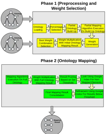
The proposed methodology is carried out in two phases (see Figure 1).
Phase 1 (Preprocessing and Weight Selection) Ontology 1 Ontology 2 Ontology Loading Percentage Selection Partial Ontology Build Up Partial Mapping Algorithm Execution On Build Up Ontology Weight Generation Weight Multiplication
With Initial Ontology Mapping Result Best Weight
Combination Selection
Phase 2 (Ontology Mapping)
Mapping Algorithms Execution On Full
Ontology
Weight Multiplication With Full Ontology
Mapping Result
Result Pruning Based on Set
Threshold
Look Using Google Index For Non-Mapped Elements
Refinement Using Google Index For Results Below
Threshold Final Mapping Result
Consolidation
Mapping Result
Figure 1. Overview of our methodology. 3.1 Phase 1: Preprocessing and Weight Selection
3.1.1 Ontology Loading
Both the Ontology 1 and Ontology 2 which are the key input for ontology mapping task are loaded. 3.1.2 Percentage Selection
This is suggested between 10 to 50 percent. 3.1.3 Partial Ontology Build Up
The value from the percentage selection step (Section 3.1.2) will be the basis to either prune both Ontology 1 and Ontology 2 or to build up a similar ontology from both the ontologies. For instance, if the selected percentage value is 10%, then 10% of elements will be selected from Ontology 1 and Ontology 2 accordingly. The elements can consist of either the concepts and their properties or just the concepts alone. It all depends on the original size of the ontologies. The output in this step will be a portion of the original ontologies. The justification of this step is to
gauge the affinity of both the ontologies in terms of string, structure and lexicon.
3.1.4 Partial Mapping Algorithm Execution on Built Up Ontology
In this step, a minimum of three algorithms of different functionality will be setup first. The three algorithms must each be for string-, structural- and lexical-based ontology mapping. Upon the setup of these three algorithms the next step would be the execution of these algorithm with the initial ontology build up described in Section 3.1.3. The final results would minimally be three different sets of mapping results each for string, structural and lexical mapping. Results of these mappings would be individual and discrete. Finally each mapping result from the individual algorithm would be summed in the form of percentage. For example, if the string mapping algorithm results in two elements being similar, and each mapping weighed 80% and 90% respectively. Thus the final summed represented for the string mapping algorithm would be 170.
3.1.5 Weight generation
Based on the number of algorithms used in Section 3.1.4, random weights will be generated. The sum of the weights would always be 1.0. For example string mapping = 0.7, structural mapping = 0.2 and lexical mapping = 0.1. The number of weights is unlimited but normally to start off we set a minimum of 20 different sets of weights. 3.1.6 Weight Multiplication with Partial Mapping Results
Each set of weights generated as described in Section 3.1.5 will be multiplied by the sum of mapping results generated as described in Section 3.1.4. The sum of mapping results in Section 3.1.4 would be normalized in percentage form.
3.1.7 Best Weight Combination Selection
The final sum generated in Section 3.1.5 would indicate the most suitable combination of weights for the mapping of Ontology 1 and Ontology 2.
This is an important step as it would have an influence in the overall mapping results which will be generated in Phase 2.
3.2 Phase 2: Ontology Mapping
3.2.1 Mapping Algorithm Execution on Full Ontology
Using the same algorithms used in Section 3.1.3, they would now be executed fully on Ontology 1 and Ontology 2 to generate individual results accordingly. The final results would be in the form of weights indicating the mapping value between elements from Ontology 1 and Ontology 2. The weight varies for each different algorithm. The nature of the mapping would be skewed according to its functionality i.e. depending on whether it was string, structural or lexical mapping.
3.2.2 Weight Multiplication with Full Ontology Results
Using the weights suggested in Section 3.1.6, each weight would now be multiplied accordingly to each result generated according to the individual algorithm. For example, if in the step described in Section 3.1.7, the weight for string mapping is 0.8. Therefore, in this step, if one of the mapping generated in Section 3.2.1 is 82%, it would now be 0.8 × 82% = 65.6%. The weight for structural and lexical mapping would also be multiplied for this element if these algorithms have also generated some results. Or else, both will be summed as 0. Finally, each individual mapped elements would have a sum result representing all three algorithms accordingly. The sum would always be below 100%.
3.2.3 Result Pruning Based on Threshold
This step concentrates on the selection of the optimal mapped element from Ontology 1 to Ontology 2. The threshold value set would be 70%. Therefore, all summed results in Section 3.2.2 that are equal or more than 70% would be selected as final mapping results.
3.2.4 Using Google Index for Non-Mapped Elements
This step is based on Normalized Google Distance (NGD) [3]. This is one way of including background knowledge for ontology mapping [8]. Basically, it gives the frequency of count for two different input keys. The result is in the form of weights where the lower the weight, the closer the two keywords are. In our methodology, NGD is applied to map elements which were not discovered in Section 3.2.1. Thus each non-mapped element in Ontology 1 will be non-mapped to a non-mapped element in Ontology 2. Here, we employ an inverse formula:
NGDi = (1 – (NGD results)) × 100%
The results would be in the form of percentage and the same threshold applied in Section 3.2.3 would be used here. Therefore, the mappings which pass the threshold limit would be selected as mapping results. We have found that this step has contributed to the discovery of the mappings that have been missed by most of the traditional algorithms used in Section 3.2.1. We will further discuss this issue in Section 4.
3.2.5 Refinement Using Google Index for Results Below Threshold
In this step, we revisit the results generated in Section 3.2.2. We relook all mappings which have failed to meet the threshold value and failed in the pruning in Section 3.2.3. By applying NGD [3] as done in Section 3.2.4, we would now apply it on these mappings. The same inverse function NGDi used in Section 3.2.4 would be applied. If the mappings exceed the threshold value, they would then be selected as part of the mapping results. 3.2.6 Final Mapping Result Consolidation
All the results generated in the Sections 3.2.3, 3.2.4 and 3.2.5 would be gathered. They would all be ordered according to either their final summed value or inverse of NGD, i.e. NGDi. Their precision, recall and F-measure values would then be calculate using the following formulas:
Precision = g eredMappin Di All g eredMappin is CorrectlyD cov cov Recall = ping CorrectMap All g eredMappin is CorrectlyD cov F-measure = ) ( 2 R P R P
Thereafter, the final mapping results could then be applied in other semantic web applications.
4 RESULTS AND DISCUSSION
Based on the described methodology, we now present the results of one mapping experiment. Both the ontologies used in this test are from the Ontology Alignment Evaluation Initiative (OAEI) [4]. The basis for using OAEI is due to the nature of its acceptance among the ontology mapping community as one of the formal standards.
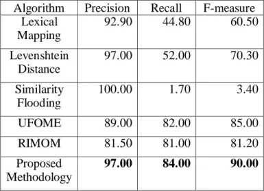
We have employed the OAEI benchmark track Ontology 101 and Ontology 301 for this test. Based on our proposed methodology, we selected the percentage value as 10%. The three different ontology mapping algorithms applied are the Levenshtein distance [5] (for string mapping), similarity flooding (for structural mapping) [6] and AgreementMaker’s lexical mapping [7] (for lexical mapping). The results are shown in Table 1.
Table 1. Result for mapping between OAEI benchmark track Ontology 101 and Ontology 301.
Algorithm Precision Recall F-measure Lexical Mapping 92.90 44.80 60.50 Levenshtein Distance 97.00 52.00 70.30 Similarity Flooding 100.00 1.70 3.40 UFOME 89.00 82.00 85.00 RIMOM 81.50 81.00 81.20 Proposed Methodology 97.00 84.00 90.00
Based on the results in Table 1, our proposed methodology performed better in every aspect of precision, recall and F-measure.
Also from the results, since most single algorithm methods like lexical mapping, Levenshtein distance and similarity flooding are focused towards only one of the property of the ontology, it has been indicated in [1, 2] that single algorithm methods do not perform as well as multi-algorithm approaches. Our proposed method was also observed to perform better than the two multi-algorithm methods, i.e. UFOME and RIMOM. Our proposed method produced better results due to the following factors:
1. Both RiMOM and UFOME’s own affinity formula have some deficiencies mainly due to its nature of restriction. In RiMOM, if the F_LS is larger than F_SS then it relies more on the lexical similarity measure and does not take much consideration on the structural mapping results. The same applies for UFOME where if the value of Sa is larger than
La, then the predictor will fully recommend the
use of just the structural-based algorithm and ignore the lexical-based algorithms. Our proposed method overcame this deficiency by not fully ignoring the lower-weighted algorithms. For example, from the results in Table 1, the weight of our method was actually
fully skewed towards the lexical algorithm, but we did not fully ignore the results of the other two algorithms (string and structural) which was beneficial in not fully eliminating results generated by them.
2. UFOME and RiMOM’s affinity calculations were done using separate algorithms which do not involve the actual mapping algorithms. This deficiency is overcame in our method by applying the step in Section 3.1.3 where we applied the exact mapping algorithms to output the weight list for the next step.
3. Application of background knowledge in the form of NGD. We found that NGD has helped in discovering mappings which were missed in the earlier steps. Additionally, the refinement step has also contributed by not fully eliminating those mappings that failed in step described in Section 3.2.3.
5 CONCLUSION
We conclude that the proposed method has contributed toward better precision, recall and F-measure in the mapping of ontologies. We have managed to overcome some of the deficiencies found in existing methods and this proves to be a positive contribution towards the relevant mapping measurements which include precision, recall and F-measures. We believe that the proposed method should be able to perform well in other tests. The biggest challenge currently is the computation of the NGD which is time consuming. We look forward towards making this more efficient.
REFERENCES
[1] J. Li, J. Tang, Y. Li, and, Q. Luo, “A Dynamic Multistrategy Ontology Alignment Framework,” IEEE Transaction on Knowledge and Data Engineering, vol. 21, no. 8, 2009, pp. 1218-1232.
[2] G. Pirró, and D. Talia, “UFOme: An Ontology Mapping
System with Strategy Prediction Capabilities,” Data and Knowledge Engineering, vol. 65, no. 65, 2010, pp. 444-471.
[3] R.L. Cilibrasi, and P.M.B. Vitanyi, “The Google Similarity Distance,” IEEE Transactions on Knowledge and Data Engineering, vol. 19, no. 3, 2007, pp. 370-383.
[4] F. Giunchiglia, M. Yatskevich, and P. Shvaiko, “Semantic matching: Algorithms and Implementation,” Journal on Data Semantics, vol. IX, 2007, pp. 1-3.
[5] A. Maedche, and S. Staab, “Measuring Similarity
Between Ontologies,” In Proceedings of the European Conference on Knowledge Acquisition and Management (EKAW), Springer, 2002, pp. 251-263.
[6] S. Melnik, H. Garcia-Molina, and E. Rahm, “ Similarity Flooding: A Versatile Graph Matching Algorithm and
Its Application to Schema Matching,” In Proceedings of the 18th International Conference on Data Engineering (ICDE ‘02), 2002, pp. 117-128.
[7] I.F. Cruz, F.P. Antonelli, and C. Stroe, “AgreementMaker Efficient Matching for Large Real-World Schemas and Ontologies,” International Conference on Very Large Databases, 2009, pp. 1586-1589.
[8] P. Shvaiko and J. Euzenat, “Ontology Matching: State
of the Art and Future Challenges, “IEEE Transactions on Knowledge and Data Engineering, vol. 25, no. 1, 2013, pp. 158-176.