Proactive Learning: Cost-Sensitive Active Learning with Multiple Imperfect Oracles

(1)

Proactive Learning: Cost-Sensitive Active Learning with

Multiple Imperfect Oracles

Pinar Donmez

Language Technologies Institute Carnegie Mellon University

5000 Forbes Ave. Pittsburgh, PA 15213, USA

Jaime G. Carbonell

Language Technologies Institute Carnegie Mellon University

5000 Forbes Ave. Pittsburgh, PA 15213, USA

ABSTRACT

Proactive learningis a generalization of active learning de-signed to relax unrealistic assumptions and thereby reach practical applications. Active learning seeks to select the most informative unlabeled instances and ask an omniscient oracle for their labels, so as to retrain the learning algorithm maximizing accuracy. However, the oracle is assumed to be infallible (never wrong), indefatigable (always answers), in-dividual (only one oracle), and insensitive to costs (always free or always charges the same). Proactive learning relaxes all four of these assumptions, relying on a decision-theoretic approach to jointly select the optimal oracle and instance, by casting the problem as a utility optimization problem subject to a budget constraint. Results on multi-oracle op-timization over several data sets demonstrate the superiority of our approach over the single-imperfect-oracle baselines in most cases.

Categories and Subject Descriptors

I.2.6 [Artificial Intelligence]: Learning—concept learning, knowledge acquisition; H.0 [General]: [Classification, cost-sensitive active learning]

General Terms

Algorithms, Experimentation

Keywords

Cost-sensitive active learning, decision-theory, multiple ora-cles

1. INTRODUCTION

In most machine learning domains, unlabeled data is avail-able in abundance, but obtaining class labels or ranking pref-erences requires extensive human effort, sometimes from ex-perts with very limited availability. For instance, it is easy

Permission to make digital or hard copies of all or part of this work for personal or classroom use is granted without fee provided that copies are not made or distributed for profit or commercial advantage and that copies bear this notice and the full citation on the first page. To copy otherwise, to republish, to post on servers or to redistribute to lists, requires prior specific permission and/or a fee.

CIKM’08, October 26–30, 2008, Napa Valley, California, USA.

to crawl the web, but much more costly to pay human an-notators to examine carefully the web documents in order to assign topics for cataloging or relevance-based judgments in a document retrieval scenario. It is also simple to col-lect images, but much harder to obtain linguistic content labels. For tasks such as classifying galaxies in the Sloan Sky Catalog, scarce expertise is required. Thus, it is crucial to design methods that will considerably reduce the labeling effort without sacrificing a significant loss of generalization accuracy.

The active learning paradigm addresses this challenge. In active learning, a few labeled instances are typically pro-vided together with a large set of unlabeled instances. The objective is first to select optimal instance(s) for an exter-nal oracle to label, and then re-run the learning method to minimize prediction error, i.e. to improve performance. The active learning task attempts to optimize learning by selecting the most informative instances to be labeled, where informativeness is typically defined as maximal expected im-provement in classification accuracy. Several studies [12, 10, 8, 4, 3] show that active learning greatly helps reduce the labeling effort in various domains. However, active learn-ing relies on unrealistic assumptions, largely swept under the proverbial carpet thus far. For instance, active learn-ing assumes there is a unique omniscient oracle. In real life, it is possible and more general to have multiple sources of information with differing reliabilities or areas of expertise. Active learning also assumes that the single oracle is perfect, always providing a correct answer when requested. In real-ity, though, an “oracle” (if we generalize the term to mean any source of expert information) may be incorrect (fallible) with a probability that should be a function of the difficulty of the question. Moreover, an oracle may be reluctant – it may refuse to answer if it is too uncertain or too busy. Fi-nally, active learning presumes the oracle is either free or charges uniform cost in label elicitation. Such an assump-tion is naive since cost is likely to be regulated by difficulty (amount of work required to formulate an answer) or other factors. In this paper, we propose proactive learning as a new approach to address these issues. Proactive learning enables active learning to reach practical applications.

We frame the proactive learning challenge as inherently a decision-theoretic problem, and focus on three scenarios. These scenarios are designed to explore different oracle types in a multi-oracle setting, i.e. oracles reluctant to give an-swers, oracles that charge non-uniform cost, and fallible or-acles that might provide wrong answers. We assume that each of these properties can be defined as a function of the

(2)

query difficulty, i.e. the level of difficulty to classify the sampled instance. Each scenario analyzes a single property; i.e. reluctance, non-uniform cost and fallibility. In multi-oracle proactive sampling, it is crucial to select the optimal data instance(s) to be queried as well as the optimal oracle. We achieved promising results on benchmark classification datasets by transforming the problem into expected utility maximization. We further assume a pre-defined and fixed budget; hence, the task becomes a constraint optimization problem. The results demonstrate the effectiveness of joint sampling of the optimal oracle-example pair as compared to sampling with respect to a single oracle.

The remainder of the paper is organized as follows: Sec-tion 2 reviews related work in active learning, and decision theory and some recent work in cost-sensitive active learn-ing. Section 3 describes in detail three scenarios we analyze and presents the proposed solution to multi-oracle proactive learning in classification. Section 4 discusses the experimen-tal setup and the results. Finally, we give our conclusions in Section 5.

2. RELATED WORK

Proactive learning is a brand new machine learning area, although there is related work in cost-sensitive active learn-ing. We review some recent work in this direction and give a broad overview of decision-theory since it provides the math-ematical tools necessary to develop algorithms for proactive learning.

Statistical decision theory is an appealing framework for proactive learning since it offers a systematic way to repre-sent cost-benefit tradeoffs, in decision-making under uncer-tainty. Uncertainty usually refers to a state of nature, which is typically unknown, but controls the sampling distribution of the observed data. A decision is defined in terms of a policyδ : Xn _→_A _{that takes an action based on a set of} observations (x1, x2, ..., xn), xi∈X. Given a non-negative loss functionL:δ→[0,+∞), each action can be associated with an expected loss (risk):

R(δ) =Eθ{L(δ(x1, ..., xn))}

whereθencodes the parameter that governs the distribution p(θ) that generates the observed data (x1, ..., xn). In

addi-tion to the risk, each acaddi-tionδ is associated with a reward (benefit), denoted by a utility functionU(δ) whose expecta-tion is taken over all possible outcomes resulting from tak-ing the action. We can denote the cost-benefit tradeoffs of different policies with a utility-risk pair (U(δ), R(δ)). The goal of decision-making is, then, to take the best action that maximizes the expected utility while minimizing the risk.

We can formulate proactive learning in the above decision-theoretic framework. The decision rule or policy corresponds to deciding whether or not to elicitate data from an oracle, i.e. querying a set of instances to obtain their labels from a human expert in a classification setting. Taking the elic-itation action introduces a certain expected reward due to the effect of the additional data on improving the learn-ing model, e.g. [10]. However, the elicitation effort incurs a cost, possibly depending on the difficulty of the task. Proac-tive learning, built with tools provided by decision theory, systematically addresses this utility-cost tradeoff for incre-mentally optimal data selection (Globally optimal selection in the general case is NP-hard).

Although active learning has received great attention among researchers, incorporating cost-benefit tradeoffs into active learning is a rather new line of investigation. Traditional ac-tive learning assumes access to unlabeled data and acquires the labels of the most informative instances at zero or uni-form cost. However, the right way is to take into account the labeling costs to design economically reliable learning meth-ods. Saar-Tsechansky and Provost [11] took a step towards that direction by proposing an active learning framework as a decision-making task. Consider the decision of initi-ating a business action such as offering a costly incentive for contract renewal. Active learning targeting improved accuracy, or in other words reduced loss, may not be suit-able for cost-effective decision making. Thus, they propose a goal-oriented strategy that selects only the examples where a small change in model estimation can affect decision-making [11]. Specifically, each unlabeled example is assigned a score that reflects the expected effect the example has on decision-making if labeled and added to the training set.

Dimitrakakis and Savu-Krohn [2] address labeling costs explicitly, where the learning goal is defined as a minimiza-tion problem over a funcminimiza-tion of the expected model perfor-mance and the total cost of labeling. This problem repre-sents a weighted combination of the generalization error of the model incurred after obtaining additional training exam-ples and the total cost associated with acquiring their labels. But, the main focus of [2] is to develop an optimal stopping criterion for sampling based on the comparison between the expected performance gain and the cost of acquiring more labels. However, the proposed stopping strategy requires the use of independent and identically distributed examples, which makes it problematic to couple with active learning.

Melville et al [6] address the cost-sensitivity in active learn-ing in the context of feature-value acquisition. In some ma-chine learning tasks, the training data has missing feature values which are often quite expensive to obtain. The goal of active feature-value acquisition is to incrementally select fea-ture values that are most cost-effective for improving learn-ing performance. Melville et al propose a selection approach based on the expected utility of acquiring the value of a fea-ture. The utility of an acquisition is defined in terms of the improvement in model accuracy per unit cost [6]. Since the true values for the model accuracy (accuracy on the unseen test data) is unknown, it is estimated by the training set accuracy. If the feature costs are assumed to be equal, this strategy is similar to the loss reduction principles presented earlier in several research studies [10, 8, 3]. Note that they still assume a single perfect oracle.

Although cost-benefit tradeoffs have started to appear in active learning, there has not yet been any notion of multi-ple oracles, with different costs, different reliabilities, differ-ent probabilities of answering, and possibly differdiffer-ent exper-tise. The general proactive learning problem requires joint maximization of the expected improvement of the learner over oracle and instance choice. In this paper, we propose a decision-theoretic approach where the most cost-effective (highest utility) oracle-instance pair is selected for data elic-itation.

3. METHODOLOGY

In this section, we present a proactive learning method for classification. We focus on three scenarios embodying the notion of multiple oracles with differing properties and

(3)

costs. Let us begin by explaining “Scenario 1”. In this sce-nario, we assume there exist one reliable oracle and one re-luctant oracle. The reliable oracle gives an answer every time it is invoked with a query, and the answer is always correct. The reluctant oracle, on the other hand, does not always provide an answer, but when it answers it does so correctly. The probability of getting an answer from the re-luctant oracle depends on the difficulty of the classification task. Not surprisingly, they charge different fees: the reliable oracle is more expensive than the reluctant one. We experi-mented with various cost combinations to simulate different real-world situations, with results in the next section.

Rather than fixing the number of instances to sample, as in standard active learning, proactive learning fixes a maxi-mum budget envelope since instances and oracles may have variable costs. Now, let us formulize the problem step by step as a joint optimization of which instance(s) to sample and which oracle to use to purchase their labels. The objec-tive is to maximize the information gain under a pre-defined budget:

maximizeE[V(S)] subject toB

whereB is the budget,S is the set of instances to be sam-pled, andE[V(S)] is the expected value of information of the sampled data to the learning algorithm. V(S) is a value function that can be replaced with any active selection cri-terion. For instance, it could be the estimated uncertainty of the current learning function atS, or a density weighted uncertainty score, or the estimated error on the unlabeled data if S is labeled and added to the training set. In our experiments, we adopted the density weighted uncertainty score proposed in [4], which significantly outperforms other strong baselines.

The above equation can be rewritten by incorporating the budget constraint into the objective function:

max S⊆U LE[V(S)]−λ( X k tk∗Ck) s.t. X k tk∗Ck=B, X k tk=|S| where the subscriptk∈ K denotes the chosen oracle from the set of oracles,K, andλis the parameter controlling the relative importance of maximizing the information and min-imizing the cost. For simplicity, we assumedλ= 1 in this paper. Ckandtkindicate the cost of the chosen oracle and the number of times it is invoked, respectively. U Lis the set of unlabeled examples, |S|is the total size of the sampled set1. Although this formulation is appealing, there is a ma-jor drawback. It is at best difficult to optimize directly due to the fact that the maximization is over the entire set of potential sampling sequences, an exponentially large num-ber. However, the learning function is updated with each additional example, which affects which examples will be sampled in the future, though we can only calculate this ef-fect after we know which examples are chosen and labeled. Thus, we cannot decide all the points to be sampled at once. A tractable alternative is a greedy approximation that will perform the optimal strategy at each round where only a sin-gle example or a small batch of examples is sampled. Now,

1_{The extension of this formulation to more than two oracles}

is straightforward.

let us see below how the greedy approach works: (x∗, k∗) = arg max

x∈U,k∈K(Ek[V(x)]−Ck) (1) Ek[V(x)] is the expected value of information of the example x with respect to corresponding oracle k. We can extend the above expectation by incorporating the probability of receiving an answer and obtain the following2_:

(x∗, k∗) = arg max

x∈U,k∈K(P(ans|x, k)∗V(x)−Ck) (2) Our goal in this scenario is to attain the maximum gain under the budget constraint. If both oracles were reliable, then the most cost-effective solution would be to use the cheapest oracle for every query. However, the cheapest or-acle may not respond to every request, especially when the query is difficult. We define a utility score, U(x, k), which is a function of the oraclekand the data pointx:

U(x, k) =P(ans|x, k)∗V(x)−Ck

When the utility is defined as above, it is often necessary to normalize the scores and the costs into the same range. In order to avoid the normalization, we re-define the utility of an example given the oracle as the information value of that example at unit cost:

U(x, k) = P(ans|x, k)∗V(x) Ck

wherek∈K (3) Unfortunately, there do not exist real-world datasets that have ground truth information on the reliability (in this case, P(ans|x, k)) of the labeling source (e.g. oracle, annotator). Therefore, we simulate the reliability as follows. We assume the amount of labeled training data available to an oracle de-termines its knowledge (expertise). For instance, the reliable (perfect) oracle resembles a system that has been trained on the entire dataset so it has perfect knowledge on each and every data point. Unlike the perfect oracle, a reluctant ora-cle has access only to a small portion of the data; therefore, it is not knowledgeable for every point. Whenever it en-counters an ambiguous data point to classify, it becomes reluctant to provide an answer. We train a classifier on a small random subset of the entire data to obtain a posterior class distributionP(y|x). For its simplicity and probabilis-tic nature, we adopted logisprobabilis-tic regression in our experiments to calculate the class posterior. The class posterior is then used for measuring uncertainty, miny∈YP(y |x), where Y

is the set of target labels. We assume that the chance of obtaining an answer from the reluctant oracle is low when the uncertainty is high and vice versa. We explain how we design the reluctance in Section 4.1 in more detail.

In order to calculate the utility as shown in Equation 3, we need to know the answer probability of the reluctant oracle. However, it is unrealistic to be given each oracle’s knowl-edge level and response characteristics apriori, so we esti-mate these properties in a discovery phase. First, we cluster the unlabeled data using kmeans clustering [5]. The number of clusters depends on the pre-defined budget available for this phase and the cost of the reluctant oracle. Second, for each cluster, we inquire the label of the data point closest to the centroid. The number of successful inquiries (i.e. the number of data points that we obtain the labels of) varies

2_{The expectation is equal to the actual value of information}

(4)

depending on the reluctance of the oracle3_{. We hypothesize}

that if the oracle does not provide the label of a data point then it is unlikely to provide the labels for the nearby points since we assume that similar points share similar posterior class probabilities. Therefore, it is reasonable to estimate the answer probability of the reluctant oracle by inquiring the labels of the cluster centroids.

For each cluster, if we obtain the label of the centroid, then we increase the answer probability of the points in this cluster. Similarly, we decrease the answer probability of the points in the clusters whose centroids we did not obtain the labels of. This step can be regarded as a belief propagation step. If we receive the label of a centroid, then we prop-agate our belief in receiving a label to similar points and vice versa. Initially, we assume the answer probability for each unlabeled point is 0.5, which indicates a random guess. Then, we adopt the following update to estimate the answer probability of each point so that it changes as a function of the proximity of the point to the cluster centroid and oracle responsiveness: ˆ P(ans|x, reluctant) = 0.5 Z ∗exp h(xct, yct) 2 ln maxd− kxct−xk kxct−xk ∀x∈Ct (4)

whereZ is a normalization constant. xct is the centroid of the clusterCtthat includesx.h(xc, yc)∈ {1,−1}is an indi-cator function which is equal to 1 when we receive the label yc for the centroid xc, and −1 otherwise. In Algorithm 1, gdenotes the number of centroids for which we receive the label. kxc−xkis the Euclidean distance between the cluster centroidxcand the pointx, andmaxd:= maxxc_´,xkxc´−xk is the maximum distance between any cluster centroid and data point.

We substitute the estimated answer probability into the utility function, i.e. Uˆ(x, k) = Pˆ(ans|x,k_C )∗V(x)

k . The joint sampling of the oracle-example pair can now be performed as shown in Algorithm 1. The algorithm works in rounds till the budget is exhausted. Each round corresponds to a single label acquisition attempt where sampling persists until obtaining a label. One important point to note here is that we need to restrain from spending too much on a single attempt by adaptively penalizing the reluctant oracle every time it refuses to answer. At any given round, if the algorithm chooses the reluctant oracle and does not receive an answer, the utility of remaining examples with respect to this oracle decreases by the amount spent thus far at this round:

ˆ

U(x, reluctant) =Pˆ(ans|x, reluctant)∗V(x) Cround

where Cround is the amount spent thus far in the given round. This penalization only applies to the reluctant ora-cle since the reliable oraora-cle always provides the label. Algo-rithm 1 selects the maximum utility examples. This frame-work leads to an incrementally optimal solution in the sense that the most useful data is sampled at the minimum cost.

In real-world, there might also be fallible oracles which answer each query, but the credibility of the answer is

ques-3_{We experimented with varying reluctance levels for a}

thor-ough investigation.

Algorithm 1Proactive Learning: Scenario 1

Input: a classifierf, labeled dataL, unlabeled dataU L,

entire budgetB, clustering budgetBC < B, two oracles, each with a costCk,k∈K={reliable, reluctant}

Output: f

- ClusterU Lintop=BC/Creluctantclusters

- Letxct be the data point closest to its cluster centroid, ∀t= 1, ..., p

- Query the labelyct for each cluster centroidxct - Identify{xc₁, ..., xcg}for which we obtain the labels - Estimate ˆP(ans|x, reluctant) via Equation 4 - UpdateL=L∪ {xct, yct}

g

t=1,U L=U L\ {xct, yct} g t=1

- cost spent so farCT =BC

whileCT < Bdo

- Trainf onL

- Initialize the cost of this roundCround = 0 and the set of queried examplesQ={}

-∀k∈K, x∈U Lestimate utility ˆU(x, k)

repeat

1. Choosek∗_{= arg max}

k∈K maxx∈U L\Q{ ˆ U(x, k)}

2. Choosex∗= arg max x∈U L\Q{

ˆ U(x, k∗)}

3. UpdateCround=Cround+Ck∗

4. Q=Q∪ {x∗_}

5. Query the labely∗with probabilityP(ans|x∗, k∗)

untillabely∗_{is obtained}

- UpdateCT =CT+Cround

- UpdateL=L∪(x∗_{, y}∗_{) and}_{U L}₌_{U L}_\₍_x∗_{, y}∗₎

end while

tionable. We simulate this setting in “Scenario 2”, where we assume two oracles; one reliable and one unreliable or-acle. The reliable oracle is the perfect oracle that always provides the correct answer to any query. The unreliable or-acle in this scenario is fallible that it may provide the wrong label for a given example. Specifically, if an example ap-proaches the decision boundary, the probability of correct classification approaches 0.5 (random guess). The proba-bility of acquiring a correct label, P(correct | x, f allible) is modeled the same way as in “Scenario 1”. The solution we propose is similar to the method introduced for “Sce-nario 1”, with slight variations. For instance, the learning method receives a random label for the queried examplex with probability 1−P(correct|x, f allible). Moreover, we use the clustering step exploiting the fallible oracle to es-timate the correctness probability P(correct | x, f allible). Similar to the previous scenario, we inquire the labels of the cluster centroids. Unlike the reluctant oracle, the fallible oracle provides the label together with its confidence. The confidence is its posterior class probability for the provided label,P(y|x). If the class posterior is within an uncertainty range, then we decide not to use the provided label since it is likely to be noisy (See Section 4.1 for details). We de-crease the correctness probability for the points in the cluster whose centroid has a class posterior in the uncertainty range. We increase the correctness probability for the points in the clusters with highly confident centroids; i.e. Pˆ(correct |

x, f allible) = 0.5 Z ∗exp ˜ h(x_ct,y_ct) 2 ln max_d−kx_ct−xk kx_ct−xk ∀x∈Ct

where ˜h(xct, yct) = −1 if minyP(y | xct) is in the uncer-tainty range, and 1 otherwise. In Algorithm 2, h denotes

(5)

entire budgetB, clustering budgetBC< B, two oracles, each with a costCk,k∈K={reliable, f allible}

Output: f

- ClusterU Lintop=BC/Cf allibleclusters

- Let xct be the data point closest to its cluster centroid, ∀t= 1, ..., p

- Query the labelyct for each cluster centroidxct - Identify {xc₁, ..., xc_h} for which the fallible oracle has high confidence

- Estimate ˆP(correct|x, f allible) - UpdateL=L∪ {xct, yct}

h

t=1,U L=U L\ {xct, yct} h t=1

- cost spent so farCT=BC

whileCT < Bdo

1. Trainf onL

2. ∀k∈K, x∈U L Uˆ(x, k) =Pˆ(correct|x,k)∗V(x)

Ck 3. Choosek∗_{= arg max}

k∈K maxx∈U L{ ˆ U(x, k)}

4. Choosex∗_{= arg max}

x∈U L{ ˆ U(x, k∗₎_}

5. UpdateCT =CT+Ck∗

6. Update L = L ∪ (x∗_{, y}∗_{) and} _{U L} ₌ _{U L} _\

(x∗_{, y}∗_{) where} _y∗ _{is the correct label with probability}

P(correct|x∗, k∗)

end while

the number of high confident centroids.

Thus far, we have only considered the settings where a uni-form fee is charged for every query by an oracle, although each oracle may charge differently. Fraud detection in bank-ing transactions is a good example for this settbank-ing. The customer records are saved in the bank database so it takes the same amount of time and effort, hence the same cost, to look up any entry in the database. On the contrary, it is pos-sible that the costs are distributed non-uniformly over the set of instances. For instance in text categorization, it might be relatively easy for an annotator to categorize a web page; hence the cost is modest. On the other hand, assigning a book into a category incurs a considerable reading time and therefore cost. Another example of a non-uniform cost sce-nario is medical diagnosis. Some diseases such as herpes are easy to diagnose. Such diagnoses are not costly since there is usually a major definitive symptom, i.e. outbreak of blisters on the skin. On the other hand, diagnosing hepatitis can be very costly since it may require blood and urine tests, CT scans, or even a liver biopsy. In “Scenario 3”, we explore the problem of deciding which instances to query for the labels when label acquisition cost varies with the instance. We as-sume two oracles one of which has a uniform and fixed cost for each query whereas the other charges according to the task difficulty. We further assume that these oracles always provide an answer and both are perfectly reliable in their answers.

In order to simulate the variable-cost (non-uniform) ora-cle, we model the cost of each example xas a function of the posterior class distributionP(y| x). We use the class posterior calculated similarly in the previous scenarios. The non-uniform costCnon−unif(x) per instance is then defined

as follows:

Cnon−unif(x) = 1−maxy∈YP(y|x)−1/|Y|

1−1/|Y|

The cost increases as the instance approaches the decision boundary and vice versa. In other words, the oracle charges based on how valuable the instance is to the learner. This may not exactly be the case in the real world, but this sets up a more challenging decision in terms of the utility-cost trade-off. The utility score in this scenario is calculated as the difference between the information value and the cost instead of the information value per unit cost4_{. This is to}

avoid infinitely large utility scores as a result of the division by small-cost. Thus, the revised utility score per oracle is given as follows:

U(x, unif) = V(x)−Cunif (5) U(x, non−unif) = V(x)−Cnon−unif(x) whereCunifis the fixed cost of the uniform-cost oracle. The pseudocode of the algorithm is given in Algorithm 3. There

entire budget B, two oracles, each with a cost Ck, k ∈

K={unif, non−unif}

Output: f

cost spent so farCT = 0

whileCT < Bdo

1. Trainf onL

2. ∀k∈K, x∈U LcalculateU(x, k) via Equation 5. 3. Choosek∗_{= arg max}

k∈K maxx∈U L{U(x, k)} 4. Choosex∗_{= arg max}

x∈U L{U(x, k

∗₎_}

5. UpdateCT=CT+Ck∗

6. UpdateL=L∪(x∗, y∗),U L=U L\(x∗, y∗)

end while

is no clustering phase in Algorithm 3 since we assume we know the cost of every instance, which is realistic for many real-world applications.

4. EXPERIMENTAL EVALUATION

In this section, we first describe the problem setup, and then present the empirical results on various benchmark datasets.

4.1 Problem Setup

In order to simulate the reliability of the labeling source (oracle), we assume that a perfectly reliable oracle resembles by a classifier trained on the entire data. An unreliable ora-cle, then, resembles a classifier trained on only a small subset of the entire data. We randomly sampled a small subset from each dataset and trained a logistic regression classifier on this sample to output a posterior class distribution. Then, we identified the instances whose class posterior falls into the uncertainty range, i.e. minyP(y|x)∈[0.45,0.5]. This range is used to filter the instances that the reluctant oracle does not answer or the fallible oracle outputs a random la-bel. One can argue that the same effect can be achieved by randomly picking such instances. However, our simulation forces a trade-off between the reliability and the information value of an instance since uncertain instances are generally informative for active learners. In order to cover a wider

4_{In general, if the cost and information value are not}

as-sessed in the same units, then they are normalized into the same range.

(6)

Table 1: Oracle Properties and Costs. BC is the

clustering budget,Bis the entire budget. Uncertain

% is the percentage of the uncertain data points. Cost Ratio is the ratio of the cost of the reliable oracle to the cost of the unreliable one.

Scenario Uncertain % Cost Ratio BC B Scenario 1 45-55% 1:3 20 300 55-60% 1:4 30 65-70% 1:5 50 Scenario 2 45-55% 1:5 20 300 55-60% 1:6 30 65-70% 1:7 50

spectrum, we varied the percentage of instances that fall into the uncertainty range [.45, .5]. The second column in Table 1 shows the different percentages used in our exper-iments. The cost of the unreliable oracle is inversely pro-portional to its reliability. We choose higher cost ratios for the fallibility scenario since receiving a noisy label should be penalized more than receiving no label at all. The tradeoff between cost and unreliability is crucial to have an incen-tive to choose between oracles rather than exploiting a single one. See Table 1 for details.

The other case we need to simulate is the uniform and non-uniform cost oracles. The cost of each instance for the variable-cost oracle is defined as a function of the class poste-rior obtained on the randomly chosen subset. This indicates a positive relationship between the difficulty of classifying an instance with its cost, which is realistic for many real-world situations. The cost of labeling each instance is known to the learning algorithm. Thus, we do not need any clustering phase in Scenario 3. We choose the cost of the uniform-cost oracle within the range of instance costs for the variable-cost oracle. Hence, the variable-costs will be comparable in the same range. We varied the fixed cost such that there is always an incentive to choose between oracles instead of fully exploit-ing a sexploit-ingle one.

We compared our method against sampling with randomly chosen oracles and sampling with a single oracle. Each base-line uses the clustering step for a fair comparative analysis. However, only our method estimates the oracle unreliability to help sampling the optimal oracle-example pair.

All the results reported in this paper are averaged over 10 runs. At each run, we start with one randomly chosen labeled example from each class. The rest of the data is con-sidered unlabeled. The learner selects one example at each iteration to be labeled, and the learning function is tested on the remaining unlabeled set once the label is obtained. The learner pays the cost of each queried example regardless of whether a label is obtained. To show the effectiveness of each method, the learning curves display the classification error versus the data elicitation cost. The budget is fixed at 300 in Scenario 1 and 2, and at 20 in Scenario 3. A small budget is enough for the latter since the cost of individual instances can be very small depending on the posterior prob-ability. We have observed that 20 is more than enough to reach a desirable accuracy in this scenario. The clustering budget, on the other hand, varies according to the unreli-ability, but is the same for each baseline under the same scenario (See Table 1). The number of clusters, though, is determined by dividing the clustering budget by the cost of

Table 2: Overview of Datasets. +/- is the

posi-tive/negative ratio. Dim is the dimensionality.

Data Face Spambase Adult VY-letter

Size 2500 4601 4147 1550

+/- 1 0.65 0.33 0.97

Dim 400 57 48 16

the oracle used during this phase. For the initial clustering phase, the unreliable oracle is used in our method and in the unreliable-oracle baselines. Thus, they obtain the same labeled data during this step, which results in the same er-ror rate. The random oracle baseline uses a fixed number of clusters, but for each cluster centroid it randomly chooses the oracle to invoke and continues until the clustering sub-budget exhausts.

4.2 Active Learning Method

We followed the density-sensitive sampling method pro-posed by [4] to evaluate the value of information of the un-labeled instances in our experiments. The method of [4] relies on conditional entropy maximization weighted by a density measure. The proposed scoring function captures not only the information content of an instance (measured by the uncertainty, i.e. minyP(y | x), but also the prox-imity weighted information content of its neighbors. The original method adopts a density-sensitive distance function and performs sampling in pairs of instances. However, we use Euclidean distance and sample a single point at a time in our experiments: U(xi) = log min yi∈{±1} {P(yi|xi,wˆ)}}+ X k6=i∈N_xi exp(−kxi−xkk22)∗ min yk∈{±1} {P(yk|xk,wˆ)} (6) [4] argues that using Euclidean distance to measure the pair-wise proximity gives comparable results and faster compu-tation.

4.3 Datasets

We study the performance of the proposed methods on various real-world benchmark datasets. The face detection dataset [9] has a total number of 393360 images, which we used a random subsample of size 2500 as in [4]. UCI-Letter is another image dataset for recognizing English capital let-ters where we labeled the letter ’V’ as the positive class and the letter ’Y’ as the negative class. This is one of the most ambiguous pairs in the data. The Spambase and the Adult datasets are also popular datasets available from the UCI Machine Learning Repository [7]. The Spambase data contains 4601 instances and 57 condition attributes. It is used to classify emails as spam and non-spam. Most of the attributes indicate whether a certain word or charac-ter appears frequently in emails. For the Adult dataset, we adopted the smaller version constructed for the IJCNN 2007 Workshop on Agnostic Learning [1]. This version has 48 fea-tures and 4147 instances in total. The task of Adult data is to discover high revenue people from the census bureau. A summary of datasets is provided in Table 2.

(7)

0 30 60 90 110 Total Cost 0.1 0.2 0.3 0.4 0.5 Classification Error Joint Random Reliable Reluctant

Spambase Cost Ratio=1:3

0 60 130 190 250 Total Cost 0.1 0.2 0.3 0.4 0.5 Joint Random Reliable

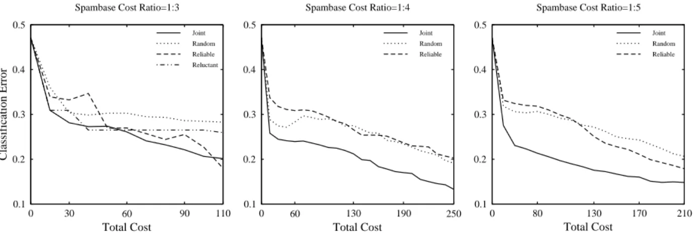
Figure 1: Performance Comparison for Scenario 1 (Reluctance) on the Spambase dataset. The cost ratio is indicated above each plot.

4.4 Empirical Evaluation

We conducted a thorough analysis to examine the perfor-mance of our method under various conditions. Due to the lack of existing work on cost-sensitive active learning with multiple oracles, we compared our method against active sampling with randomly chosen oracles and active sampling with a single oracle. We denote our method of jointly opti-mizing oracle and instance selectionJoint, the random sam-pling of oracles Random. Reliable, Reluctant, and Fallible refer to the corresponding single oracle baseline.

We next clarify why the maximum cost of data elicitation, shown in Figures 1-8, differ in various tasks and scenarios. The results are averaged over 10 runs for each experiment. At each run, the total number of iterations to spend the entire budget may differ depending on how the budget is allocated between oracles. In order to take the average of the results, we rely on the minimum number of iterations attained over 10 runs for each experiment. This ensures that all runs equally contribute to the average. This also results in different maximum elicitation costs smaller than the budget for different experiments. Nevertheless, theJoint strategy outperforms the others even after spending only a small amount in most cases.

Figure 1 shows the results for the reluctance scenario on the Spambase dataset. Each plot indicates a different cost ratio. Our method outperforms the others on every case while the performance gap increases with the cost ratio. This is largely because the oracle differences leave more room for improvement via oracle selection in the latter case. When the unreliability gets higher, the reluctant oracle tends to spend almost the entire budget on a single label acquisition attempt. This leads to acquiring only a small amount of labeled data; hence, its poor performance. As a result, we do not report the reluctant oracle baseline except in its best case, the 1 : 3 cost ratio.

Figures 2 and 3 show the comparison between our method and the other baselines for Scenario 1 on the Adult and VY-Letter datasets, respectively. For the Adult dataset, our Joint method outperforms the others when the cost ratio is 1 : 3 while it tracks the best performer for the other cost ratios. Generally,Jointtracks the best performer when the best performer is a clear winner for the entire operating range. This pattern is also evident in Figure 3 for the cost

ratio 1 : 3. For the other cost ratios, Joint significantly outperforms the other baselines on the VY-Letter dataset.

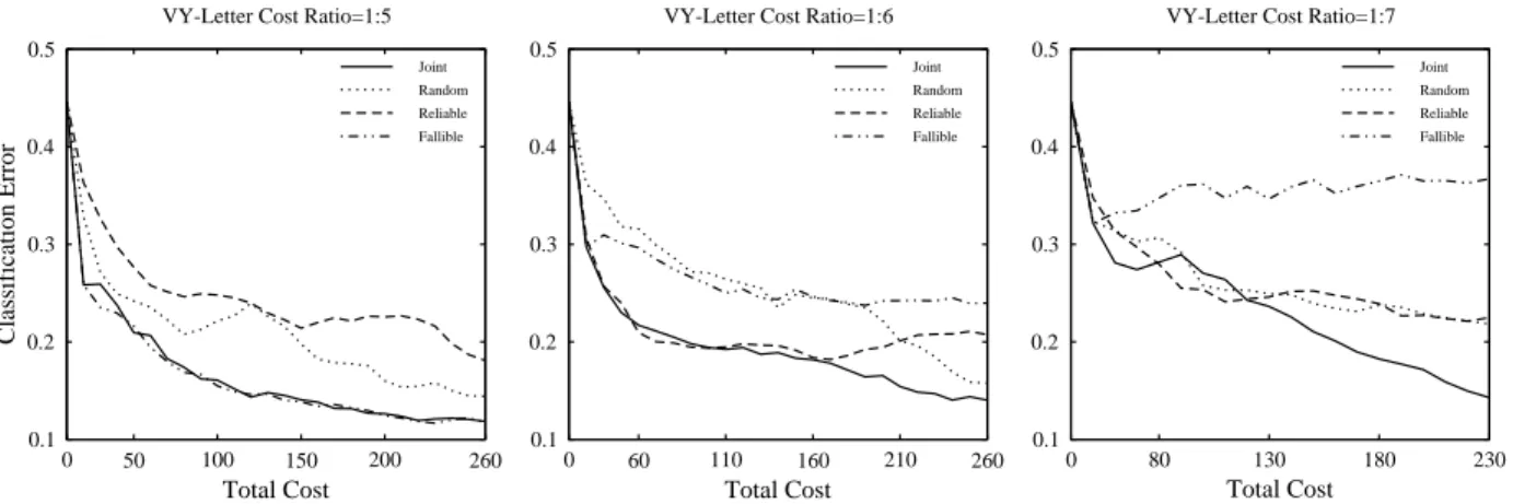
Figure 4 compares the performances for Scenario 2 on the VY-Letter dataset. The Fallible oracle in this scenario per-forms poorly when the relative cost ratio is high. As shown in Table 1, the cost ratio increases with the number of unre-liable instances. In other words, a higher cost ratio indicates a more unreliable oracle. Thus, the Fallible oracle may in-crease the classification error with more labeled data since the labels are increasingly likely to be noisy. This pattern is especially evident in Figure 4 for the cost ratio 1 : 7. On the other hand,Jointstrategy is quite effective for reducing the error in this scenario, indicating that it is capable of re-ducing the risk of introre-ducing noisy data through strategic selection between oracles.

We present the rest of the results in Table 3. Due to space constraints, we selected a representative cost ratio for each dataset. The values in bold correspond to the winning methods. Joint wins frequently (i.e. 10 out of 16) and is a close runner-up on the other cases.

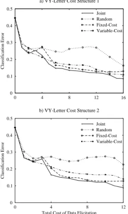
Figures 5, 7 and 8 present the evaluation results when the cost varies non-uniformly across the set of instances. We ex-perimented with different assignments of the fixed cost, each of which is a function of the average instance cost, denoted avg, for the non-uniform cost oracle. We present two rep-resentative assignments for each dataset: Cost1:= avg/1.5 and Cost2:= avg/2. The remaining cost values are not in-cluded since they are similar to those reported here. On the Face and the Spambase datasets,Jointis the best performer throughout the full operating range. Moreover, Joint pre-dominantly outperforms the others on the VY-letter dataset. The performance difference betweenJointand each baseline is also statistically significant based on a paired two-sided t-test (p < 0.01). For the Adult dataset, both cost cases performed equivalently; hence, there was no opportunity for “Joint” to optimize further.

In order to investigate if the initial clustering phase helps all the baselines, we re-ran each baseline excluding the clus-tering step. In this case, there is no separate clusclus-tering budget; hence, the entire budget is spent in rounds for data elicitation. Figure 6 compares each baseline with the clus-tering restriction on the Spambase dataset for Scenario 1. Every baseline significantly benefits from clustering, with

(8)

0 30 50 80 100 Total Cost 0.2 0.3 0.4 0.5 0.6 Classification Error Joint Random Reliable Reluctant

Adult Cost Ratio=1:3

0 80 130 180 220 260 Total Cost 0.2 0.3 0.4 0.5 0.6 Joint Random Reliable

Figure 2: Performance Comparison for Scenario 1 (Reluctance) on the Adult dataset. The cost ratio is indicated above each plot.

0 60 120 180 230 Total Cost 0 0.1 0.2 0.3 0.4 0.5 Classification Error Joint Random Reliable Reluctant

VY-Letter Cost Ratio=1:3

Figure 3: Performance Comparison for Scenario 1 (Reluctance) on the VY-Letter dataset. The cost ratio is indicated above each plot.

Table 3: Results on different datasets for two scenarios. Cost column shows the total cost spent to reach the corresponding error rate. The best result on each row is given in bold.

Error Rate

Scenario Dataset & Cost Ratio Cost Joint Random Reliable Unreliable

Scenario 1 Face & 1:4

60 0.195 0.294 0.347 0.188 120 0.179 0.275 0.261 0.192 180 0.144 0.201 0.163 0.178 240 0.119 0.137 0.118 0.168 Scenario 2 Face & 1:5 70 0.250 0.294 0.468 0.343 130 0.233 0.298 0.298 0.271 190 0.165 0.330 0.193 0.250 250 0.152 0.215 0.153 0.233 Spambase & 1:7 70 0.285 0.335 0.264 0.369 120 0.243 0.328 0.289 0.373 170 0.185 0.311 0.279 0.357 220 0.151 0.281 0.262 0.337 Adult & 1:6 70 0.334 0.386 0.302 0.363 130 0.309 0.358 0.295 0.362 190 0.288 0.300 0.284 0.350 250 0.269 0.278 0.281 0.342

(9)

0 50 100 150 200 260 Total Cost 0.1 0.2 0.3 0.4 0.5 Classification Error Joint Random Reliable Fallible

0 60 110 160 210 260 Total Cost 0.1 0.2 0.3 0.4 0.5 Joint Random Reliable Fallible

0 80 130 180 230 Total Cost 0.1 0.2 0.3 0.4 0.5 Joint Random Reliable Fallible

Figure 4: Performance Comparison for Scenario 2 (Fallibility) on the VY-Letter dataset. The cost ratio is indicated above each plot.

A A A A A A A A A 0 4 8 12 17 0 0.1 0.2 0.3 0.4 0.5 Classification Error Joint A A Random Fixed-Cost Variable-Cost a) Face Cost Structure 1

A A A A A A A A 0 3 6 10 14

Total Cost of Data Elicitation 0 0.1 0.2 0.3 0.4 0.5 Classification Error Joint A A Random Fixed-Cost Variable-Cost b) Face Cost Structure 2

Figure 5: Comparison of different algorithms under non-uniform cost structures (Scenario 3) on Face. a) (Top panel) Fixed-Cost oracle has Cost1 b) (Bottom panel) Fixed-Cost oracle has Cost2.

the biggest boost in improvement occurring for the Reluc-tant oracle. Hence, both the baselines and the “Joint” strat-egy benefit from the diversity-based sampling via clustering in their initial steps. Without pre-clustering, the Reluctant oracle is prone to spend too much on a single elicitation at-tempt due to unsuccessful labeling requests. It can, however, maximize the chance of receiving a label through diversity sampling during the clustering step instead of getting stuck in one round for a single label.

A A A A A A A A A A 0 5 10 14 18 0 0.1 0.2 0.3 0.4 0.5 Classification Error Joint A A Random Fixed-Cost Variable-Cost a) Spambase Cost Structure 1

A A A A A A A 0 3 7 10 13

Total Cost of Data Elicitation 0 0.1 0.2 0.3 0.4 0.5 Classification Error Joint A A Random Fixed-Cost Variable-Cost b) Spambase Cost Structure 2

Figure 7: Comparison of different algorithms under non-uniform cost structures (Scenario 3) on Spam-base. a) (Top panel) Fixed-Cost oracle has Cost1 b) (Bottom Panel) Fixed-Cost oracle has Cost2.

5. CONCLUSIONS

In this paper, we proposed proactive learning to over-come the unrealistic assumptions of active learning. We introduced three scenarios that analyze the effect of mul-tiple imperfect oracles with differing properties and costs on selective sampling. The proposed methods formulated in a decision-theoretic framework rely on expected utility maxi-mization across oracle-example pairs. The empirical results demonstrate the effectiveness of this approach against

(10)

ran-0 30 60 90 110 Total Cost 0.2 0.25 0.3 0.35 0.4 0.45 0.5 Classification Error w/o Clustering w/ Clustering Reluctant Oracle 0 30 60 90 110 Total Cost 0.1 0.2 0.3 0.4 0.5 w/o Clustering w/ Clustering Reliable Oracle 0 30 60 90 110 Total Cost 0.2 0.25 0.3 0.35 0.4 0.45 0.5 w/o Clustering w/ Clustering Random Oracle

Figure 6: Change in performance of each baseline with and without clustering on Spambase. The type of baseline is given in the title. The cost ratio is 1:3.

A A A A A A A A A 0 4 8 12 16 0 0.1 0.2 0.3 0.4 0.5 Classification Error Joint A A Random Fixed-Cost Variable-Cost a) VY-Letter Cost Structure 1

A A A A A A A 0 4 8 12

Total Cost of Data Elicitation 0 0.1 0.2 0.3 0.4 0.5 Classification Error Joint A A Random Fixed-Cost Variable-Cost b) VY-Letter Cost Structure 2

Figure 8: Comparison of different algorithms un-der non-uniform cost structures (Scenario 3) on VY-Letter. a) (Top panel) Fixed-Cost oracle has Cost1 b) (Bottom panel) Fixed-Cost oracle has Cost2.

dom oracle selection and exploitation of a single oracle, even the best one. This paper takes a step towards filling in a gap between active learning and real-world tasks to make active learning reach practical applications. As future work, we will investigate relocating resources in scenarios with no apriori information about oracle properties to optimize the cost-benefit tradeoff.

6. ACKNOWLEDGMENTS

This material is based in part upon work supported by the Defense Advanced Research Projects Agency (DARPA)

under Contract No. NBCHD030010.

7. REFERENCES

[1] Agnostic learning vs. prior knowledge challenge and data representation discovery workshop, 2007. IJCNN ’07.

[2] C. Dimitrakakis and C. Savu-Krohn. Cost-minimising strategies for data labelling: optimal stopping and active learning.Foundations of Information and Knowledge Systems, FOIKS 2007, 2007.

[3] P. Donmez and J. G. Carbonell. Optimizing estimated loss reduction for active sampling in rank learning. International Conference on Machine Learning, ICML ’08, 2008.

[4] P. Donmez and J. G. Carbonell. Paired sampling in density-sensitive active learning.International

Symposium on Artificial Intelligence and Mathematics, 2008.

[5] J. Hartigan and M. Wong. A k-means clustering algorithm.Applied Statistics, 28.

[6] P. Melville, M. Saar-Tsechansky, F. Provost, and R. Mooney. Economical active feature-value

acquisition through expected utility estimation.KDD ’05 Workshop on Utility-based data mining, 2005. [7] D. Newman, S. Hettich, C. Blake, and C. Merz. UCI

repository of machine learning databases, 1998. University of California, Irvine, Dept. of Information and Computer Sciences.

[8] H. Nguyen and A. Smeulders. Active learning with pre-clustering.ICML ’04, pages 623–630, 2004. [9] T. Pham, M. Worring, and A. Smeulders. Face

detection by aggregated bayesian network classifiers. Pattern Recognition Letters, 23.

[10] N. Roy and A. McCallum. Toward optimal active learning through sampling estimation of error reduction.ICML ’01, pages 441–448, 2001.

[11] M. Saar-Tsechansky and F. Provost. Decision-centric active learning of binary-outcome models.Journal of Information Systems Research, 18.

[12] S. Tong and D. Koller. Support vector machine active learning with applications to text classification. ICML ’00, pages 999–1006, 2000.

[13] G. M. Weiss and Y. Tian. Maximizing classifier utility when training data is costly.ACM SIGKDD

Proactive Learning: Cost-Sensitive Active Learning with Multiple Imperfect Oracles