Comparative analysis of support vector machine, maximum likelihood and neural network classification on multispectral remote sensing data

Comparative Analysis of Support Vector Machine,

Maximum Likelihood and Neural Network

Classification on Multispectral Remote Sensing Data

Asmala Ahmad

, Ummi Kalsom Mohd Hashim

,

Othman Mohd

, Mohd Mawardy Abdullah

Centre for Advanced Computing Technology (C-ACT) Fakulti Teknologi Maklumat Dan Komunikasi (FTMK)

Universiti Teknikal Malaysia Melaka Melaka, Malaysia

Hamzah Sakidin

Department of Fundamental and Applied Sciences Universiti Teknologi PETRONAS

Perak, Malaysia

Abd Wahid Rasib

Tropical Map Research Group, Department of Geoinformation

Faculty of Geoinformation and Real Estate Universiti Teknologi Malaysia

Johor, Malaysia

Suliadi Firdaus Sufahani

Fakulti Sains Gunaan dan Teknologi Universiti Tun Hussein Onn Malaysia

Johor, Malaysia

Abstract—Land cover classification is an essential process in

many remote sensing applications. Classification based on supervised methods have been preferred by many due to its practicality, accuracy and objectivity compared to unsupervised methods. Nevertheless, the performance of different supervised methods particularly for classifying land covers in Tropical regions such as Malaysia has not been evaluated thoroughly. The study reported in this paper aims to detect land cover changes using multispectral remote sensing data. The data come from Landsat satellite covering part of Klang District, located in Selangor, Malaysia. Landsat bands 1, 2, 3, 4, 5 and 7 are used as the input for three supervised classification methods namely support vector machines (SVM), maximum likelihood (ML) and neural network (NN). The accuracy of the generated classifications is then assessed by means of classification accuracy. Land cover change analysis is also carried out to identify the most reliable method to detect land changes in which showing SVM gives a more stable and realistic outcomes compared to ML and NN.

Keywords—Land cover; change detection; remote sensing; training set; supervised classification

I. INTRODUCTION

In the early days, land cover information was obtained by manual surveying on foot or land vehicles. This approach had been adopted in many parts of the world for decades but later was found impractical for some circumstances. For instance, for large and remote areas, such approach requires a lot of time and logistically expensive.

Aerial photography was next introduced where land cover information was captured using a camera mounted on an aircraft. This had allowed land cover information to be recorded in a much shorter time. However, such approach was found weather-dependent besides exposing aircraft operators to air accidents. With advancement of recent space technologies,

remote sensing satellite was then introduced where land cover information can be captured using sensors mounted on satellites. This is a far better option than the aerial photography as huge land cover information are now able to be obtained continuously, globally and with a relatively cheaper cost.

Such technology enables monitoring of land covers to be effectively carried out at different times [1],[2],[3]. Consequently, this allows changes in land cover that occurred in a certain period of time to be detected. Changes in land cover associated with human activities and natural phenomenon is an important indication for accurate decision making to be made particularly related to agricultural, environmental and urban management [4],[5],[7].

Land cover classification is an essential process in assessing land cover changes. Classification task is performed by assigning each pixel in an image to the correct land cover type. Classification based on supervised methods, which utilise training pixels, has been preferred by researchers in detecting changes in land cover at different parts of the world [7],[8],[9]. Nevertheless, in most cases, only a single supervised method has been considered and evaluated whereas not many attempted to use more than one methods and comparatively analysed their performances [10],[11],[12]. Consequently, the performance of a method with respect to others is not known in-depth leading to a naïve understanding on the issue [13],[14],[15]. This is particularly true for Tropical land covers such as those found in Malaysia [16],[17],[18].

This study attempts to perform land cover classification using maximum likelihood (ML), neural network (NN) and support vector machines (SVM) to assess land cover changes in Klang District, located in Selangor, Malaysia. The performance of each of these methods is to be evaluated based on classification accuracy and land cover change analysis

[19],[20],[22],[23]. Comparative analysis is eventually performed among these methods by making use of these performance measures.

II. LAND COVER CLASSIFICATION

Classification is the process of assigning a pixel to a particular type of land cover [24], [25],[26]. Classification uses data which are mathematically known as a measurement vector or feature vector from an acquisition system. It aims to assign a pixel associated with the measurement at a specific position to a particular class. The classes are defined from supporting data, such as maps and ground data for areas of interest. Two approaches of classification can be considered i.e. unsupervised and supervised classification. Unsupervised classification is a two-step operation of grouping pixels into clusters based on the statistical properties of the measurements, and then labelling the clusters with the appropriate classes [21]. Supervised classification starts from a known set of classes, learns the statistical properties of each class and then assigns the pixels based on these properties [22]. In this study supervised classification was chosen due to the following criteria:

 Simplicity – the practicality of using a large amount of data. This should involve a smaller number of procedures but should produce reasonably accurate and standard results,

 Accuracy – the ability to select important land covers with an acceptable accuracy, i.e. each pixel will be assigned to the correct land cover on the ground. The performance of the method should not be easily affected by factors such as the complexity of land covers, topographic conditions, etc. and

 Objectivity – not involving tuning by a user to improve performance. The generated classification works straight away without needing any adjustment in terms of the number of classes, training pixels, etc.

The three supervised classification schemes to be considered in this study are support vector machine (SVM), maximum likelihood (ML) and neural network (NN).

A. Support Vector Machine (SVM)

SVM is performed by making use of an efficient hyperplane searching technique that uses minimal training area and therefore consumes less processing time [3],[7]. It is a non-parametric method but capable of developing efficient decision boundaries and therefore can minimize misclassification. SVM works by identifying the optimal hyperplane and divides the data points into two classes. There will be an infinite number of hyperplanes and SVM will select the hyperplane with maximum margin. The margin indicates the distance between the classifier and the training points.

B. Maximum Likelihood (ML)

In ML, the distribution for each class in each band is assumed to be normal and the probability a given pixel belongs to a specific class [4],[27] is calculated based on this assumption. Each pixel is then assigned to the class that has the

highest probability. Classification is performed by calculating the discriminant functions for each pixel in the image.

C. Neural Network (NN)

In NN, classification is carried out in the conditions where land covers are not linearly separable in the original spectral space. This is performed by making use of multiple nonlinear activation functions at different layers [5]. The training pixels help in identifying the threshold and weight vector connected in the network.

III. METHODOLOGY

This study involves three phases i.e. data pre-processing, data processing and land cover change analysis. Landsat satellite data were obtained from the Malaysian Remote Sensing Agency (MRSA) and United States Geological Survey (USGS) involving Landsat data acquired in 1998, 2000 and 2005. In data pre-processing, we initially calibrated the data where pixel‘s raw digital number is converted into radiance:

L =gain* DN + bias (1)

Where L is the pixel value in radiance, DN is the cell value digital number, gain is the gain value for a specific band, and bias is the bias value for a specific band. Atmospheric correction is the process of removing the effects of the atmosphere on the reflectance values of images taken by satellite. Atmospheric Effects are caused by scattering and absorption of EM radiation in the atmosphere and have significant effects mainly on visible and infrared bands that tend to affect processing and interpretation of images. Geometric correction is the process of correcting the data for geometric distortion due to non-systematic error occurred. This was done by initially applying geometric correction on a base-data selected from one of the Landsat base-data and then registering all other data onto the base-data. Subset was carried out for the selected area within the image, since satellite data usually covers a very large area.

Subsequently, we performed a preliminary assessment to understand the performance of ML, SVM and NN when the size of the training pixels was varied. Such situation may occur when carrying out land cover change detection later due to haze and cloud issues [6],[7]. For this purpose, 1998 Landsat-5 bands 1, 2, 3, 4, 5 and 7 that sense in visible and near infrared wavelengths were used. Band 6 that senses in thermal wavelengths was omitted due to its irrelevancy to this study. Visual interpretation of the Landsat data, aided by a land cover map, was carried out and 11 main classes were identified, viz. coastal swamp forest, dryland forest, oil palm, rubber, industry, cleared land, urban, coconut, bare land sediment plumes and water. Regions of interest (ROIs) associated with the training were determined by choosing one or more polygons for each class based on visual interpretation of the land cover map and Landsat data. This was assisted by region growing technique in which pixels within polygons were grown to neighbouring pixels based on a threshold, i.e. the number of standard deviations away from the mean of the drawn polygons. Pixels for the 11 classes of land cover were determined based on the land cover map. Sampling was carried out by means of stratified random sampling technique. This was done by dividing the population (the entire classification image) into

homogeneous subgroups (the ROI for individual classes) and then taking a simple random sample in each subgroup. 11 training sets were extracted based on percentage of pixels within the ROIs, viz. 10%, 20%, 30%, 40%, 50%, 60%, 70%, 80% and 90%. Each of training sets was fed into each of the classifiers i.e. ML, NN and SVM where the accuracy of the classification was assessed by means of percentage classification accuracy [6], [7].

In data processing, we applied the ML, SVM and NN classification to the 2000 and 2005 data to determine land cover changes throughout these dates [28],[29]. Similarly, 11 land covers were considered i.e. coastal swamp forest, dryland forest, oil palm, rubber, industry, cleared land, urban, coconut, bare land, sediment plumes and water.

The results can be categorised into three phases, i.e. data pre-processing, data processing and land cover change detection analysis, as follows.

D. Data Pre-processing

The classification results for 10% through 90% training set size were evaluated by using confusion matrices to assess the capability of SVM, ML and NN in classifying the 11 predefined land covers. In order to better see these classes, suitable colours were assigned to the land covers: coastal swamp forest (green), dryland forest (blue), oil palm (yellow), rubber (cyan), industry (thistle), cleared land (purple), urban

(red), coconut (maroon), bare land (orange), sediment plumes (dark green) and water (white). Classification and reference (ground truth) data set were compared among all cases.

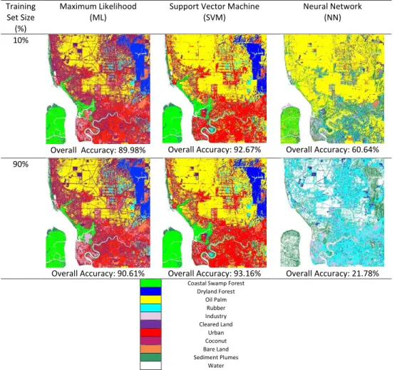
Fig.1 shows the classification result by applying ML, NN and SVM method for two extreme cases 10% (the smallest) and 90% (biggest) training set sizes. Visually, based on qualitative visual analysis of the land cover colour distribution, it is obvious that ML and SVM are able to classify more land covers compared to NN for both cases. For 10% training set size, NN recognizes most land covers as oil palm in which is not the case. Similarly, for 90% training set size, NN produces unrealistic scenario by assigning most land covers as rubber.

For ML, it is noticeable for both cases, coconut is found far too abundant along the sea side areas and encroaches markedly towards the inland areas in which likely to be an ambiguous case. In other words, it is likely that misclassification occurs between oil palm and coconut in ML classification. It is likely that these results are due to the similarities of spectral properties between oil palm and coconut. It is also found that there is a discrepancy between the far abundant coconut near the dryland forest for the 10% compared to the 90% training pixel. For SVM, it can be seen that the distribution of classes is rather consistent for the 10% and 90% training pixels indicating that the performance of SVM is not much influenced by the training set size.

Fig. 1. Land Cover Classification using ML, NN and SVM when using 10% and 90% Training Set Sizes.

Training Set Size

(%)

Maximum Likelihood (ML)

Support Vector Machine (SVM)

Neural Network (NN) 10%

Overall Accuracy: 89.98% Overall Accuracy: 92.67% Overall Accuracy: 60.64% 90%

Overall Accuracy: 90.61% Overall Accuracy: 93.16% Overall Accuracy: 21.78% Coastal Swamp Forest

Dryland Forest Oil Palm Rubber Industry Cleared Land Urban Coconut Bare Land Sediment Plumes Water

In terms of quantitative analysis, for both (10%, 90%) training set sizes, SVM (92.67%, 93.16%) has the highest overall accuracy, followed by ML (89.98%, 90.61%) and NN gives the lowest accuracy (60.64%, 21.78%). SVM and ML have a similar performance trend where the classification accuracy for 90% is higher than the 10% training set size. However, the performance is vice versa for NN. The accuracy differences of the extreme cases for SVM, ML and NN are found to be 0.49%, 0.62% and 38.87% respectively. This shows that SVM has a higher stability when making use of relatively small numbers of training data sets compared to ML and NN. Thus, ML can be regarded as the method that depends much on the accuracy and sufficiency of the training pixels. NN has been known as a method that not only depending on training pixels or learning the rules but its process is also affluence by the network topology that encompasses the hidden layer and interconnections.

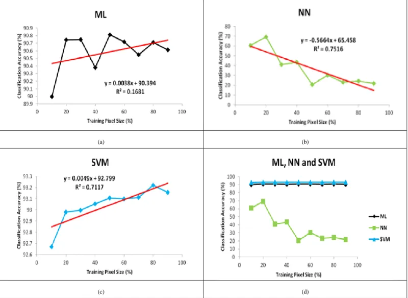
To understand further the trend of the classification accuracy with respect to the training pixel size, linear regression analysis was applied to each of the classifications. Fig. 2(a) shows a plot of classification accuracy versus training

set size for ML. Although fluctuating, there is somewhat an increasing trend when classification accuracy is plotted against training set size. The linear regression analysis gives R2 of 0.1681 indicating weak positive correlation between the classification accuracy and training set size. Fig. 2(b) shows a plot of classification accuracy versus training set size for NN. It can be seen there is a decreasing trend between classification accuracy and training set size. The regression analysis gives R2 of 0.7516 indicating a somewhat strong negative trend between the classification accuracy and training set size. Fig. 2(c) shows a plot of classification accuracy versus training set size for SVM. There is a noticeable increasing trend between classification accuracy and training set size. The regression analysis gives R2 of 0.7117 indicating a rather strong positive correlation between the classification accuracy and training set size. Fig. 2(d) shows plot of classification accuracy versus training set size for ML, NN and SVM. Clearly, SVM and ML have the higher stability compared to NN in which the accuracy drops drastically as training size increases. However, SVM noticeably outperforms ML due to much higher R2 besides having the least difference in classification accuracy as training set size increases.

(a) (b)

(c) (d)

ML and SVM shows a more realistic classification of land covers compared to NN. However, SVM was found more stable due to not much being affected by varying training set size compared to ML when the size of the training pixels was varied; its accuracy is not much affected compared to ML. SVM also have shown a more realistic land cover area distribution changes compared to ML related to the real scenario.

E. Data Processing

Table I shows land cover area in km2 classified using SVM, ML and NN for the 2000 and 2005 data while Table II shows land cover changes in km2 from 2000 to 2005 based on SVM, ML and NN classification. The land covers are classified into 11 classes; coastal swamp forest (CSF), coconut (C), urban (U), industry (I), dryland forest (DLF), oil palm (OP), bare land (BL), rubber (R), cleared land (CL), water (W) and sediment plumes (SP). For SVM classification, the major conversions are the bare land area and urban area. During the 5-year period, the bare land has decreased by 118 km2. Urban area experienced the highest increase, i.e. 107 km2. This is followed by the coastal land forest 15 km2, oil palm 29.3 km2increase, cleared land 13.5 km increase and industry 6.5 km2increase. Other significant changes have been declines in the sediment plumes 3.9 km2, water 3.4 km2, rubber 0.93 km2and coconut 0.8 km2.

TABLE I. LAND COVERS CLASSIFIED USING SVM, ML AND NN FOR 2000 AND 2005 Land Cover Total of Area (km2₎ 2000 2005 SVM ML NN SVM ML NN CSF 45.80 37.60 0.00 61.55 48.20 331.25 SP 17.93 34.89 0.00 14.00 18.19 0.00 U 52.81 79.25 5.66 160.32 161.36 0.00 I 2.80 29.57 0.00 9.27 45.96 9.83 W 54.65 41.72 52.21 51.26 46.74 0.11 DLF 72.43 44.70 122.57 27.90 18.30 143.19 BL 131.85 84.76 2.39 12.87 20.37 15.82 CL 3.90 9.40 0.00 17.39 14.62 39.97 OP 150.99 100.51 145.98 180.29 164.76 0.00 R 3.02 10.21 32.97 2.09 1.11 0.00 C 4.12 67.70 178.53 3.37 0.68 0.14

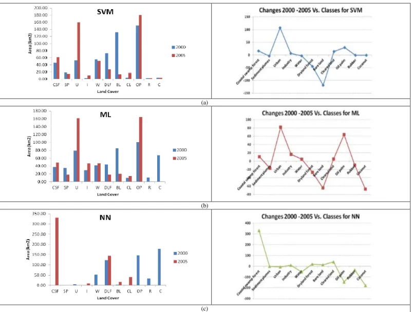
Fig. 3 shows land cover changes from 2000 to 2005 based on area for SVM, ML and NN. SVM and ML shows quite a similar trend that is more realistic but not for NN. Further analysis is carried out to analyse closely the changes based on each land cover from 2000 to 2005.

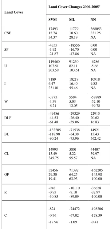
TABLE II. LAND COVER CHANGES DETECTED USING SVM, ML AND NN FOR THE YEAR 2000 TO 2005

Land Cover

Land Cover Changes 2000-2005a

SVM ML NN CSF 17493 15.74 34.37 11779 10.60 28.19 368053 331.25 NA SP -4355 -3.92 -21.87 -18556 -16.70 -47.86 0.00 0.00 NA U 119460 107.51 203.59 91230 82.11 103.61 -6286 -5.66 NA I 7189 6.47 231.01 18219 16.40 55.46 10918 9.83 NA W -3773 -3.39 -6.21 5584 5.03 12.05 -57889 -52.10 -99.78 DLF -49486 -44.53 -61.48 -29329 -26.40 -59.06 22915 20.62 16.83 BL -132205 -118.98 -90.24 -71538 -64.38 -75.96 14921 13.43 562.42 CL 14993 13.49 345.75 5801 5.22 55.57 44407 39.97 NA OP 32456 29.30 19.41 71392 64.25 63.93 -162205 -145.98 -100.00 R -948 -0.93 -30.85 -10110 -9.10 -89.09 -36628 -32.97 -100.00 C -824 -0.76 -17.96 -74472 -67.02 -1.09 -198206 -178.39 -0.41 a.

(a)

(b)

(c)

Fig. 3. Land Cover Changes from 2000 to 2005 Detected using SVM (top), ML (middle) and NN (bottom). F. Land Cover Change Detection Analysis

Fig. 4 shows land cover areas for the year 2000 versus 2005 classified using SVM, ML and NN for (a) coastal swamp forest, (b) sediment plumes, (c) urban, (d) industry, (e) water, (f) dryland forest, (g) bare land, (h) cleared land, (i) oil palm, (j) rubber and (k) coconut. For coastal swamp forest, SVM and ML gives a more realistic results compared to NN due to the conversion mainly from coastal swamp forest to oil palm which is the most important commercial crop for Malaysia. For sediment plumes, conversion to coastal swamp forest shown by SVM and NN are seen more realistic, due to the nature of both land covers that is located near to water body, compared to conversion to mainly urban shown by ML. For urban, SVM shows a more realistic outcome due to the very little conversion to oil palm as a highly commercial crop compared to conversion to sediment plumes and bare land by ML and NN respectively. For industry, a little conversion to urban by SVM is more realistic compared to sediment plumes and water in ML and non-existence of industry in NN. For water, a very little conversion to coastal swamp forest by SVM is more realistic compared to conversion to industry in ML and

non-existence of water in NN. For dryland forest, conversion to urban in SVM is more realistic than conversion to sediment plumes in ML and non-existence of dryland forest in NN. For bare land, conversion to mainly urban and oil palm in SVM is more realistic than conversion to mainly sediment plumes in ML and conversion coastal swamp forest in NN. For cleared land, conversion to urban and oil palm in SVM is more realistic compared to conversion to sediment plumes that occurred in ML and conversion to coastal swamp forest that occurred in NN. For oil palm, conversion to urban in SVM is more realistic compared to sediment plumes in ML and conversion to coastal swamp forest in NN. For rubber, conversion to oil palm and urban in SVM is more realistic compared to conversion to sediment plumes that occurred in ML and conversion to coastal swamp forest that occurred in NN.

We carried out a different test to determine the realistic scores for each of the methods. ‗1‘score is given for each land cover that gives sensible changes that took place during 2000 to 2005. Based on the land changes that are detected by three methods, SVM possess 100% scores due to the sensible

changes detected for all land covers i.e. coastal swamp forest, dryland forest, oil palm, rubber, industry, cleared land, urban, coconut, bare land sediment plumes and water. ML and NN score 27% each due to the sensible changes for coastal swamp forest and water for the former while sediment plumes and coconut for the latter.

The superiority of SVM over ML and NN is mainly due to less being influenced by the size of training sets. This is likely due to the behaviour of SVM that performs classification by

assigning pixel to the correct land cover type by making use of the hyperplane and maximum margin. This leads to the assignment of pixels to the correct land covers and therefore misclassification is minimised. The classification process consequently affects the change detection assessment.

Further research is required to determine how these methods would perform on study areas that differ in terms of land use, vegetation cover, topography, and other variables.

SVM ML NN (a) (b) (c) (d) (e)

SVM ML NN (f) (g) (h) (i) (j) (k)

Fig. 4. Land Cover areas for the Year 2000 Versus 2005 Classified using SVM, ML and NN for (a) Coastal Swamp Forest, (b) Sediment Plumes, (c) Urban, (d) Industry, (e) Water, (f) Dryland Forest, (g) Bare Land, (h) Cleared Land, (i) Oil Palm, (j) Rubber and (k) Coconut.

IV. CONCLUSION

In this study, a comparative analysis of SVM, ML and NN has been performed by means of classification accuracy and change detection analysis. Landsat satellite images of Klang

have been used in the study. The study have encompassed three main process: data pre-processing, data processing and land cover change detection analysis. In data pre-processing, Landsat images have been chosen due to its multispectral capability. Spatial subset and spectral subset have been

performed to resize the images based on the study area and identify the suitable bands in the images respectively. Three methods have been performed in the classification process i.e. SVM, ML and NN. In data processing, the classifications have been performed to the year 2000 and 2005 data where SVM, ML and NN are used to identify the changes in land cover throughout this period. Finally, land cover change analysis has been implemented by analysing the distribution of land cover areas for the year 2000 and 2005 classified using SVM, ML and NN. Overall, SVM produces a more sensible and realistic results compared to ML and NN mainly due to less being influenced by the size of training sets.

ACKNOWLEDGMENT

The Authors are grateful to Universiti Teknikal Malaysia Melaka (UTeM) for providing the student research funding through the UTeM Zamalah Scheme.

REFERENCES

[1] A. Singh, ―Review Article Digital change detection techniques using remotely-sensed data,‖ International Journal of Remote Sensing, vol. 10, no. 6, pp. 989-1003, 1989.

[2] K.R. Manjula, J. Singaraju J. and A.K. Varma, ―Data preprocessing in multi-temporal remote sensing data for deforestation analysis,‖ Global Journal of Computer Science and Technology Software & Data Engineering, vol. 13, no. 6, pp. 1-8, 2013.

[3] N.IS. Bahari, A. Ahmad and B.M. Aboobaider, ―Application of support vector machine for classification of multispectral data,‖ 7th IGRSM International Remote Sensing & GIS Conference and Exhibition. IOP Conf. Series: Earth and Environmental Science 20, 2014.

[4] A. Ahmad and S. Quegan, ―The effects of haze on the spectral and statistical properties of land cover classification,‖ Applied Mathematical Sciences, vol. 8, no. 180, pp. 9001-9013, 2014.

[5] A. Ahmad and S. Quegan, ―Haze modelling and simulation in remote sensing satellite data,‖ Applied Mathematical Sciences, vol. 8, no. 159, pp. 7909-7921, 2014.

[6] M.F. Razali, A. Ahmad, O. Mohd and H. Sakidin, ―Quantifying haze from satellite using haze optimized transformation (HOT),‖ Applied Mathematical Sciences, vol. 9, no. 29, pp. 1407 – 1416, 2015.

[7] U.K.M. Hashim and A. Ahmad, ―The effects of training set size on the accuracy of maximum likelihood, neural network and support vector machine classification,‖ Science International-Lahore, vol. 26, no. 4,. pp. 1477-1481, 2014.

[8] K. Islam, M. Jashimuddin, B. Nath, T. Kumar Nath, ―Land use classification and change detection by using multi-temporal remotely sensed imagery: The case of Chunati wildlife sanctuary, Bangladesh,‖ The Egyptian Journal of Remote Sensing and Space Science, vol. 21, no. 1, pp. 37-47, 2018.

[9] K. Islam, M. Jashimuddin, B. Nath and T.K. Nath, ―Quantitative assessment of land cover change using landsat time series data : case of Chunati Wildlife Sanctuary (CWS), Bangladesh,‖ Int. J. Environ. Geoinformatics, vol. 3, pp. 45-55, 2016.

[10] J. Jayanth, T. Ashok Kumar, S. Koliwad and S. Krishnashastry. ―Identification of land cover changes in the coastal area of Dakshina Kannada district, South India during the year 2004–2008,‖ Egypt. J. Remote Sens. Space Sci., vol. 19, pp. 73-93, 2016.

[11] L.N. Kantakumar and P. Neelamsetti, ―Multi-temporal land use classification using hybrid approach,‖ Egypt. J. Remote Sens. Space Sci., vol. 18, pp. 289-295, 2015.

[12] A.M. Lal and S.M. Anouncia, ―Semi-supervised change detection approach combining sparse fusion and constrained k means for multi-temporal remote sensing images,‖ Egypt. J. Remote Sens. Space Sci. vol. 18, pp. 279-288, 2015.

[13] H.M. Mosammam, J.T. Nia, H. Khani, A. Teymouri and M. Kazemi, ―Monitoring land use change and measuring urban sprawl based on its spatial forms: the case of Qom city,‖ Egypt. J. Remote Sens. Space Sci., vol. 20, no. 1, pp. 103-116, 2017.

[14] J.S. Rawat and M. Kumar, ―Monitoring land use/cover change using remote sensing and GIS techniques: a case study of Hawalbagh block, district Almora, Uttarakhand, India,‖ Egypt. J. Remote Sens. Space Sci., vol. 18, pp. 77-84, 2015.

[15] S. Sinha, L.K. Sharma and M.S. Nathawat, ―Improved Land-use/Land-cover classification of semi-arid deciduous forest landscape using thermal remote sensing,‖ Egypt. J. Remote Sens. Space Sci., vol. 18, pp. 217-233, 2015.

[16] C. Liping, S. Yujun and S. Saeed, ―Monitoring and predicting land use and land cover changes using remote sensing and GIS techniques—A case study of a hilly area, Jiangle, China,‖ PLoS ONE, vol. 3, no. 7, pp. 1-23, 2018.

[17] S.K. Singh, P.B. Laari, S. Mustak, P.K. Srivastava and S. Szabó, ―Modelling of land use land cover change using earth observation data-sets of Tons River Basin, Madhya Pradesh, India,‖ Geocarto Int., pp. 1-34, 2017.

[18] A.K. Hua, ―Land use land cover changes in detection of water quality: a study based on remote sensing and multivariate statistics,‖Journal of Environmental and Public Health, pp. 1-12, 2017.

[19] Y. Gao, Z. Liang, B. Wang, Y. Wu and P. Wu, ―Wetland change detection using cross-fused-based and normalized difference index analysis on multitemporal Landsat 8 OLI,‖ Journal of Sensors, vol. 2018, pp. 1-8, 2018.

[20] B. Wang, J. Choi, S. Choi, S. Lee, P. Wu and Y. Gao, ―Image fusion-based land cover change detection using multi-temporal high-resolution satellite images,‖ Remote Sensing, vol. 9, no. 804, pp. 1-19. 2017. [21] D. Renza, E. Martinez, I. Molina, and D.M.L. Ballesteros,

―Unsupervised change detection in a particular vegetation land cover type using spectral angle mapper,‖ Advances in Space Research, vol. 59, no. 8, pp. 2019–2031, 2017.

[22] R. Singh, M. Singha, S. Singh, D. Pal, N. Tripathi and R. Singh, ―Land use/land cover change detection analysis using remote sensing and GIS of Dhanbad distritct, India,‖ Eurasian Journal of Forest Science, vol. 6, no. 2, pp. 1-12, 2018.

[23] S.M. Arafat, K. Abutaleb, E. Farg, M. Nabil1 and M. Ahmed, ―Identifying land use change trends using multi-temporal remote sensing data for the New Damietta City, Egypt,‖ Journal of Geography, Environment and Earth Science International, vol. 14, no. 3, pp. 1-12, 2018.

[24] A, Sahar, ―Performance of spectral angle mapper and parallelepiped classifiers in agriculture hyperspectral image,‖ International Journal of Advanced Computer Science and Applications, vol. 7, no. 5, pp. 55-63, 2016.

[25] A, Sahar, ―Hyperspectral image classification using unsupervised algorithms,‖ International Journal of Advanced Computer Science and Applications, vol. 7, no. 4, pp. 198-205, 2016.

[26] A. Kulkarni and A. Shrestha, ―Multispectral image analysis using decision trees,‖ International Journal of Advanced Computer Science and Applications, vol. 8, no. 6, 11-18, 2017.

[27] A.K. Thakkar, V.R. Desai, A. Patel and M.B. Potdar, ―Post-classification corrections in improving the ―Post-classification of land use/land cover of arid region using RS and GIS: The case of Arjuni watershed, Gujarat, India,‖ The Egyptian Journal of Remote Sensing and Space Science, vol. 20, no. 1, pp. 79-89, 2017.

[28] M.D.C. Janiola and G.R. Puno, ―Land use and land cover (LULC) change detection using multi-temporal landsat imagery: A case study in Allah Valley Landscape in Southern, Philippines,‖ J. Bio. Env. Sci., vol. 2, no. 2, pp. 98-108, 2018.

[29] M.Z. Iqbal and M.J Iqbal, ―Land use detection using remote sensing and gis (A case study of Rawalpindi Division),‖ American Journal of Remote Sensing, vol. 6, no. 1, pp. 39-51, 2018.