Heft 264 Jieru Yan
Nonlinear estimation of short time
precipitation using weather radar and
surface observations
Nonlinear estimation of short time precipitation using
weather radar and surface observations
von der Fakultät Bau- und Umweltingenieurwissenschaften der
Universität Stuttgart zur Erlangung der Würde einer
Doktor-Ingenieurin (Dr.-Ing.) genehmigte Abhandlung
vorgelegt von
Jieru Yan
aus Zhengzhou, China
Hauptberichter:
Prof. Dr. rer.nat. Dr.-Ing. András Bárdossy
Mitberichter:
Prof. Dr. ir. Remko Uijlenhoet
Tag der mündlichen Prüfung:
28.11. 2018
Institut für Wasser- und Umweltsystemmodellierung
der Universität Stuttgart
Heft 264 Nonlinear estimation of short
time precipitation using weather
radar and surface observations
von
Dr.-Ing.
Jieru Yan
Eigenverlag des Instituts für Wasser- und Umweltsystemmodellierung
der Universität Stuttgart
Bibliografische Information der Deutschen Nationalbibliothek
Die Deutsche Nationalbibliothek verzeichnet diese Publikation in der Deutschen
Nationalbibliografie; detaillierte bibliografische Daten sind im Internet über
http://www.d-nb.de abrufbar
Yan, Jieru
:
Nonlinear estimation of short time precipitation using weather radar and surface
observations, Universität Stuttgart. - Stuttgart: Institut für Wasser- und
Umweltsystemmodellierung, 2018
(Mitteilungen Institut für Wasser- und Umweltsystemmodellierung, Universität
Stuttgart: H. 264)
Zugl.: Stuttgart, Univ., Diss., 2018
ISBN 978-3-942036-68-9
NE: Institut für Wasser- und Umweltsystemmodellierung <Stuttgart>: Mitteilungen
Gegen Vervielfältigung und Übersetzung bestehen keine Einwände, es wird lediglich
um Quellenangabe gebeten.
Herausgegeben 2018 vom Eigenverlag des Instituts für Wasser- und
Umweltsystem-modellierung
First of all, I would like to express my gratitude to Prof. Andr´as B´ardossy, who sets a good example of how a scientific scholar should look like. I was always impressed by his endless ideas of solving tricky problems, all attacking the key of the problems in a relatively simple manner, which certainly requires experience, abundant knowledge reserve and innovation. I was also impressed by his enthusiasm in work and his optimistic attitude upon encountering prob-lems temporarily without a solution. As a knowledgeable scholar, he values the academic exchanges of multiple forms, not only restricted to the a narrow range of the specialty, but he wishes to know more about the relevant fields, which alters my original mindset and could form a ever-lasting influence on me in the following research life.
My special thanks to Prof. Remko Uijlenhoet from University of Wageningen, for his support and valuable suggestions during my study. I sincerely thank Prof. Manfred Joswig for being the chair of both my qualifying and doctoral examination.
I would like to extend my thanks to my former colleague Sebastian H¨orning, who was also the second supervisor of my Master’s thesis. His patience in ex-planation, brilliant guidance and support at that time have sparked my interest in academic research.
I am very grateful to have a bunch of colleagues: Astrid Lemp, Jochen Seidel, Dirk Schlabing, Thomas M¨uller, Micha Eisele, Faizan Anwar, etc; my two Chi-nese colleagues Ning Wang and Naibin Song; and my former colleagues Yingchun Huang and Tobias Mosthaf. All of them have helped me now and then. Alto-gether, they form a community of good atmosphere in the institute for Mod-elling Hydraulic and Environmental Systems, the department of Hydrology and Geohydrology.
And thanks to my friends, who keep life interesting, share good memories with me, accompany and help me through hard time during these years’ of stay in Germany.
I would like to acknowledge the China Scholarship Council, the Chinese Ministry of Education’s non-profit organization, provides me financial support during my PhD study. I would also like to acknowledge ENWAT International Doctoral Program of University of Stuttgart for providing a very good academic frame-work for my study. A lot of thanks to the course director Dr.-Ing. Gabriele M. Hartmann, who offers me lots of detailed information and valuable advice.
whether it is pleasant or hard time in life; my mother, the cheerful, open-minded and peaceful lady, always gives me unconditional love, care, understanding and encouragement in the far afield China; and finally, my soon-to-born daughter, who makes me stronger and brings me happiness as a mother.
List of Figures IV
List of Tables VI
List of Abbreviations VII
Abstract IX
Kurzfassung XI
1 Introduction 1
1.1 Motivation . . . 1
1.2 Two challenges in radar hydrology . . . 2
1.2.1 Extrapolation of radar reflectivity to the surface . . . 2
1.2.2 Conversion of radar reflectivity to precipitation intensity . . . 3
1.3 Scope and structure of this thesis . . . 8
2 Study area and data 9 2.1 Study area and gauge data . . . 9
2.2 Radar data . . . 10
2.2.1 Basics of weather radar . . . 10
2.2.1.1 Radar equation . . . 10
2.2.1.2 Wavelength of weather radar . . . 12
2.2.2 Problems arised in quantitative precipitation estimation . . . 13
2.2.2.1 Clutter . . . 14
2.2.2.2 Attenuation . . . 15
2.2.2.3 Anomalous Propagation . . . 17
2.2.2.4 Uncertainty in Z-R relationship . . . 19
2.2.2.5 Signal fluctuation . . . 22
2.2.2.6 Radial degradation of map quality . . . 22
2.2.3 General aspects of local radar data . . . 24
3 Wind displacement 27 3.1 Introduction . . . 27
3.2 Two kinds of wind displacement . . . 28
3.2.1 Horizontal displacement . . . 28
3.3 Quantification of wind displacement . . . 32
3.3.1 Quantification of the displacement between two radar imageries . . . 32
3.3.1.1 Literature . . . 32
3.3.1.2 Algorithm description . . . 33
3.3.1.3 Examples . . . 35
3.3.2 Quantification of the displacement between a radar imagery and sur-face observations . . . 36
3.3.3 Correlation of the horizontal and the vertical displacement . . . 37
3.3.4 Stability of wind displacement . . . 40
3.4 Integration of wind displacement . . . 42
3.4.1 Literature . . . 42
3.4.2 Wind information integrated radar rainfall accumulation . . . 43
3.4.3 Examples . . . 44
4 Surface precipitation estimation 48 4.1 Literature on the radar-gauge merging techniques . . . 48
4.2 Quantification of the conflict between gauge and radar data . . . 51
4.2.1 Application — test on the agreement of gauge and radar data . . . 52
4.3 The expected field . . . 54
4.3.1 Algorithm description . . . 54
4.3.2 Example . . . 57
4.3.3 The influence ofg(x)on the resultant expected field . . . 60
4.3.4 The relative independence of the expected rainfall field on the mea-surement height of radar imagery . . . 63
4.3.5 The insufficiency of the expected rainfall field . . . 67
5 Improvement by geostatistical methods 69 5.1 Introduction . . . 69
5.2 External drift kriging . . . 72
5.3 Residual kriging . . . 74
5.4 Comparison of different geostatistical methods . . . 75
5.5 Cross validation . . . 79
6 Improvement by simulation 83 6.1 Introduction . . . 83
6.2 Prerequisite and requirements on the simulated realizations . . . 84
6.2.1 Prerequisite . . . 84
6.2.2 Requirements on the simulated realizations . . . 84
6.3 Random mixing . . . 85 6.3.1 Literature . . . 85 6.3.2 Algorithm . . . 86 6.3.3 Algorithm supplement 1 . . . 91 6.3.4 Algorithm supplement 2 . . . 92 6.3.5 Examples . . . 94
6.3.5.2 Use multiple shifted rainfall fields as the input . . . 99 6.4 Phase Annealing . . . 101 6.4.1 Literature . . . 101 6.4.1.1 Simulated annealing . . . 101 6.4.1.2 Phase randomization . . . 103 6.4.2 Algorithm . . . 104 6.4.3 Examples . . . 108
6.5 Comparison of random mixing and phase annealing . . . 110
6.6 Cross validation . . . 111
7 Conclusions 113
1.1 The variability of drop size distribution with time . . . 6
1.2 The variability of drop size distribution with height . . . 7
2.1 Location and discretization of the study domain . . . 9
2.2 Electromagnetic spectrum . . . 12
2.3 Schematic diagram of various sources of spurious echoes in weather radar data 14 2.4 Modification of rain areas caused by raindrop attenuation . . . 15
2.5 Occurrence principle of anomalous propagation echo . . . 17
2.6 Example 1 showing the vertical variability of Z-R relationship . . . 20
2.7 Example 2 showing the vertical variability of Z-R relationship . . . 21
2.8 Relative positions of the study domain in the radar polar coordinates . . . 23
2.9 Radar network of DWD . . . 25
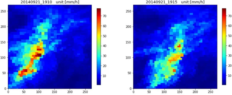
3.1 Radar imageries of precipitation intensity sampled every 5 min . . . 29
3.2 Example 1 showing the existence of vertical displacement . . . 31
3.3 Example 2 showing the existence of vertical displacement . . . 31
3.4 Quantification of the horizontal wind displacement . . . 35
3.5 Quantification of the vertical wind displacement . . . 36
3.6 Graphical illustration of the procedure to test on the correlation of the vertical and the horizontal wind displacement . . . 39
3.7 Downscaled radar maps of rain rate by the nearest neighbor method. . . 45
3.8 The two contributors of the interpolated radar map . . . 45
3.9 Comparison of radar rainfall accumulations with and without the integration of wind information . . . 46
3.10 The smooth transition of the magnitude of precipitation rate . . . 47
4.1 The agreement of radar and gauge data measured by rank correlation . . . . 53
4.2 Radar rainfall fields showing the non-representativeness of surface observations 56 4.3 Surface precipitation estimates without and with wind information integrated 57 4.4 Marginal distribution functions involved in the generation of the expected rainfall field . . . 58
4.5 Scaled alternatives of functiong(x) . . . 61
4.6 The expected rainfall fields for the same event obtained by applying different conversion functionsg(x) . . . 63
4.7 Radar maps measured at different altitudes as the data source of the expected rainfall fields (Exp.1) . . . 65
4.8 The expected rainfall fields resulting from radar maps measured at different altitudes (Exp.1) . . . 65
4.9 Radar maps measured at different altitudes as the data source of the expected
rainfall fields (Exp.2) . . . 66
4.10 The expected rainfall fields resulting from radar maps measured at different altitudes (Exp.2) . . . 67
4.11 Insufficiency of the expected rainfall field at the observational locations . . . . 68
5.1 Scaled variograms derived from the expected rainfall fields . . . 74
5.2 Estimates of surface precipitation by ordinary kriging, external drift kriging and residual kriging (Exp. 1) . . . 77
5.3 Estimates of surface precipitation by ordinary kriging, external drift kriging and residual kriging (Exp. 2) . . . 78
6.1 The fulfillment of the similarity requirement indicated by different iterations of random mixing . . . 92
6.2 Ring effect of sinc interpolation . . . 93
6.3 Modified searching strategy of random mixing . . . 94
6.4 Mean field of 100 random mixing realizations using the expected rainfall field as the input . . . 95
6.5 Random mixing realizations using the expected rainfall field as the input . . . 96
6.6 Marginal distribution functions of 100 random mixing realizations . . . 96
6.7 Standard deviation map over 100 random mixing realizations . . . 97
6.8 Example showing the problem of using the expected rainfall field as the input 98 6.9 The expectated realization (Exp.1) . . . 99
6.10 The expectated realization (Exp.2) . . . 100
6.11 The expectated realization (Exp.3) . . . 100
6.12 The expectated realization (Exp.4) . . . 101
6.13 The marginal distribution functions of the simulated realizations by phase annealing . . . 108
6.14 The expected realization by the algorithm of phase annealing . . . 109
6.15 Map of standard deviation over the simulated realizations by the algorithm of phase annealing . . . 110
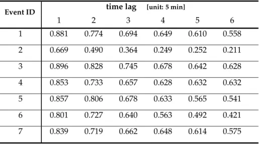
1.1 Specification of MRR system . . . 5 2.1 Comparison of different radar bands . . . 13 2.2 Specification of Radar T ¨urkheim and Radar Feldberg . . . 24 3.1 Basic information of the seven selected rainfall events with long wet periods . 38 3.2 The correlation of the horizontal and the vertical wind displacement . . . 40 3.3 Stability of the vertical wind displacement . . . 41 3.4 Stability of the horizontal wind displacement . . . 41 4.1 The agreement between radar (wind information integrated/non-integrated
precipitation accumulation) and gauge data . . . 53 4.2 Non-representativeness of surface observations . . . 56 4.3 Error statistics showing the benefit of integrating wind information in surface
precipitation estimation . . . 60 4.4 The influence of functiong(x)on the resultant expected rainfall field . . . 62
5.1 Descriptive statistics of the gauge data used in the cross validation of the geo-statistical methods . . . 80 5.2 Cross validation results of OK, EDK and RK. . . 81 5.3 Cross validation results of RK using the wind integrated and non-integrated
fields as the second variable. . . 82 6.1 Descriptive statistics of the gauge data used in the cross validation of the two
simulation methods . . . 112 6.2 Cross validation results of random mixing and phase annealing. . . 112
VPR Vertical profile of reflectivity DSD Raindrop size distribution MRR Micro rain radar
EM Electromagnetic PPI Plan position indicator m. a. g. Meter above the ground
QPE Quantitative precipitation estimation anaprop Anomalous propagation
AP Anomalous propagation VRG Vertical refractivity gradient
DWD German weather service (Deutscher Wetterdienst) Tur Radar T ¨urkheim
Fbg Radar Feldberg
BLUE Best linear and unbiased estimate ME Mean error
RMSE Root mean square error KGE Kling Gupta Efficiency EDK External drift kriging RK Residual kriging OK Ordinary kriging
Rain gauges are the foundation in hydrology to collect rainfall data, however, gauge obser-vations alone are limited at representing the complete rainfall distribution. On the other hand, weather radar can provide complete rainfall distribution at high temporal and spatial resolution, yet concerns about the biases in radar rainfall estimates hamper the direct use of radar data in hydrological applications. Thus, merging radar measurements and rain gauge observations for surface precipitation estimation, by exploiting the strength and minimizing the weaknesses of each method, is in an area of active research.
Among all the sources of errors of radar rainfall estimates, the uncertainty in the relationship between radar reflectivity Z and rainfall rate R, namely the Z-R relationship, is regarded as a massive source of uncertainty. There is a whole branch of studies on delivering an accurate Z-R relationship based on different drop size distributions, rainfall regimes and geographical locations. The focus of this study is not to derive an accurate Z-R relationship, but to correct the radar rainfall estimates by the available surface observations nonlinearly. Specifically, radar data are used in the relative magnitudes, as a quantile map to indicate the spatial pattern of precipitation. A marginal distribution function is generated based on surface observations and the collocated radar quantiles, whereby the quantile map can be transformed to a precipitation map.
It is a common practice to construct radar-gauge pairs by assuming vertical and instant falling of the hydrometeors onto the ground. Obviously, the assumption is invalid on many occasions, as it ignores a significant fact that it takes time for the hydrometeors to reach the ground and during the descending, the hydrometeors are very likely to be drifted by the wind, especially with a large measurement height and with the existence of snow. The effect of wind drift can result in great discrepancy of radar and gauge data if the vertical collocation is assumed, especially for domains of small size and for events with convective behavior. To tackle this, a method to quantify the wind effect is proposed and the result of the quantification is integrated in surface precipitation estimation.
The spatial pattern of precipitation changes along the vertical distance. The change in the spatial pattern can be induced by many factors, such as uniform movement of the field, fur-ther development of precipitation below the radar measurement height, evaporation, non-uniform movement of the field, etc. The quantification scheme for the wind effect proposed in this study considers an overall migration of the field. It is assumed that the entire field moves uniformly with a single vector. The other factors causing the vertical variation of the spatial pattern cannot be captured by the scheme. To remediate the situation, random changes in the spatial pattern are allowed. Two conditional simulation methods, random mixing and phase annealing, are employed to generate realizations of surface precipitation.
Niederschlagsmesser sind in der Hydrologie die Grundlage f ¨ur die Sammlung von Re-gendaten. Allerdings sind Pegelbeobachtungen in der Darstellung der vollst¨andigen Niederschlagsverteilung eingeschr¨ankt. Ein Wetterradar kann eine vollst¨andige Nieder-schlagsverteilung mit hoher zeitlicher und r¨aumlicher Aufl ¨osung liefern, dennoch behin-dern Bedenken bez ¨uglich des systematischen Fehlers hinsichtlich der Sch¨atzung des Radar-Niederschlags die direkte Nutzung von Radardaten in hydrologischen Anwendungen. Da-her ist das Zusammenf ¨uhren von Radarmessungen und von Beobachtungen des Nieder-schlagsmessers zur Niederschlagssch¨atzung der Oberfl¨ache durch Ausnutzung der St¨arke und Minimierung der Schw¨achen jeder Methode Gegenstand aktiver Forschung.
Unter allen Fehlerquellen von Radarregensch¨atzungen wird die Unsicherheit in der Beziehung zwischen der Radarreflektivit¨at Z und der Niederschlagsrate R, der soge-nannten Z-R-Beziehung, als massive Unsicherheitsquelle angesehen. Es gibt eine ganze Reihe von Studien ¨uber die Bereitstellung einer genauen Z-R-Beziehung, die auf unter-schiedlichen Tropfengr ¨oßenverteilungen, Niederschlagsregimen und geografischen Stan-dorten basiert. Der Fokus der vorliegenden Arbeit liegt nicht darauf, eine genaue Z-R-Beziehung abzuleiten, sondern die Radar-Niederschlagssch¨atzungen durch die verf ¨ugbaren Oberfl¨achenbeobachtungen nichtlinear zu korrigieren. Hier werden Radardaten in rela-tiven Gr ¨oßen verwendet, als Quantilkarte, um das r¨aumliche Muster des Niederschlags anzuzeigen. Eine Grenzverteilungsfunktion wird auf der Grundlage von Oberfl¨achen-beobachtungen und den zusammengestellten Radarquantilen generiert, wodurch die Quan-tilkarte in eine Niederschlagskarte umgewandelt werden kann.
Es ist allgemein ¨ublich, Radarmesspaare zu konstruieren, indem man das vertikale und so-fortige Fallen der Hydrometeore auf den Boden annimmt. Offensichtlich ist die Annahme in vielen F¨allen ung ¨ultig, da sie eine signifikante Tatsache ignoriert, n¨amlich dass die Hydrom-eteore Zeit ben ¨otigen, um den Boden zu erreichen, und dass die HydromHydrom-eteoren w¨ahrend des Abstiegs mit hoher Wahrscheinlichkeit vom Wind verweht werden, insbesondere bei einer großen Messh ¨ohe und bei Vorhandensein von Schnee. Der Effekt der Winddrift kann zu einer großen Diskrepanz der Radar- und Messger¨atdaten f ¨uhren, wenn von der ver-tikalen Kollokation ausgegangen wird, insbesondere f ¨ur kleine Dom¨anen und f ¨ur Ereignisse mit konvektivem Verhalten. Um dies zu bew¨altigen, wird eine Methode zur Quantifizierung des Windeffekts vorgeschlagen, und das Ergebnis der Quantifizierung wird in die Nieder-schlagssch¨atzung der Oberfl¨ache integriert.
Das r¨aumliche Niederschlagsmuster ¨andert sich entlang der vertikalen Entfernung. Die Ver¨anderung kann durch viele Faktoren hervorgerufen werden, beispielsweise durch eine gleichm¨aßige Bewegung des Feldes, Weiterentwicklung des Niederschlags unterhalb der Radarmessh ¨ohe, Verdampfung, ungleichm¨aßige Bewegung des Feldes usw. Das in dieser
Studie vorgeschlagene Quantifizierungsschema f ¨ur den Windeffekt betrachtet eine gesamte Migration des Feldes. Es wird angenommen, dass sich das gesamte Feld gleichm¨aßig mit einem einzigen Vektor bewegt. Die anderen Faktoren, die die vertikale Variation des r¨aum-lichen Musters verursachen, k ¨onnen durch das Schema nicht erfasst werden. Zur Behe-bung dieser Situation sind zuf¨allige ¨Anderungen im r¨aumlichen Muster zugelassen. Zwei Simulationsmethoden, Random Mixing und Phase Annealing, werden zur Erzeugung von Oberfl¨achenniederschl¨agen eingesetzt.
1.1 Motivation
“It may be possible therefore to determine with useful accuracy the intensity of rainfall at a point quite distant (say 100 km) by the radar echo from that point.” With that sentence Marshall et al. [1947] launched the quest for the hydrological use of radar. And despite the tremendous progress, this request still continues [Fabry, 2015]. As it is generally accepted, radar is apt at measuring the spatial patterns of reflectivity at some altitude where the mea-surement has been taken. Although with some uncertainties, the spatial patterns of reflec-tivity aloft can be assumed as the estimates of the spatial distribution of the instantaneous precipitation intensity.
If the quantitative precipitation estimates are not needed, and the precipitation monitoring is only required on a qualitative or semiquantitative level, then radar is a naturally superb tool: the plan position indicator (PPI) of reflectivity which is not affected by gross errors, such as bright band contamination or attenuation, can already provide the needed adequate infor-mation [Fabry, 2015]. And a large proportion of radar users fit in this category. However in terms of hydrological uses of radar, precise measurements of precipitation accumulation at the ground surface over a relevant time period are required. The branch of hydrology seeking to realize the goal of quantitative precipitation estimation using weather radar is known asradar hydrology.
Hydrological uses of weather radar include, for instance, climatological services, manage-ment of rivers and sewers, precision agriculture and early detection of flood for protection of life and property [Fabry, 2015]. All of these applications have common requirements on data accuracy, but the latter imposes additional challenge because of the special demand on the rapidness. The techniques dedicated to solve the last problem are usually referred to as
nowcasting, to make forecasts over relatively short time periods from a few minutes to a few hours.
As for the precision in terms of the precipitation measurement over a time period on the ground, rain gauges is unapproachable, because they are the only device that measures ground rainfall directly. Although rain gauges are poor in terms of measuring short-term precipitation accumulation or instantaneous precipitation intensity, the measurement error diminishes rapidly as the integration time increases. While the opposite rule applies for weather radar. Radar measures the reflectivityZ induced by precipitation, which is then related to precipitation intensityRusing a proper Z-R relation. And radar rainfall is accu-mulated on the relevant instantaneous precipitation intensity maps. Thus, the estimation error builds up as the accumulation time increases.
According to Fabry [2015], the persistent challenge of radar hydrology consists in transform-ing a time sequence of instantaneous estimates of reflectivity aloft into an unbiased estima-tion of precipitaestima-tion accumulaestima-tion at the ground surface, which necessitates a systematic fight against every source of error that can build up in time. As hidden in the description of the challenge in radar hydrology, the time sequence of instantaneous estimates of reflectivity measured at a certain altitude above the ground are to be translated to precipitation accu-mulation at the surface. The distance between radar measurement height and estimation height is a very important factor which hampers the quantitative precipitation estimation by weather radar.
1.2 Two challenges in radar hydrology
The study focuses on two challenges in radar hydrology, extrapolation of radar reflectivity to the ground surface and conversion of radar reflectivity to precipitation intensity. The two challenges are discussed in the following sections.
1.2.1 Extrapolation of radar reflectivity to the surface
Meteorological induced reflectivity can change considerably with height, especially in cold season precipitation, when the radar beam starts to intercept the 0◦
isotherm, resulting in considerable biases (e.g. [Joss et al., 1990]; [Fabry et al., 1992]). A mapping function is therefore required to transform the reflectivity measured aloft to the one that would have been observed at the ground surface.
A common practice is to assume the establishment of a vertical profile of reflectivity (VPR), and further assumption on the stability of the VPR at different radar range. Then, the single VPR is used for the extrapolation of reflectivity aloft onto the ground, given the elevation angle of the antenna and the beam width of the radar to calculate the measurement height of each radar range (e.g. [Joss et al., 1990], etc). However, the correction procedure using a single VPR is questionable because of the strong assumption about the uniform VPR. The net effect of the correction scheme is to add a range-dependent constant number of dBs to all echoes independent of their magnitude (e.g. [Steiner et al., 1995], etc). Yet in practice, a magnitude-independent single VPR rarely exists. The VPR can vary with precipitation intensity, and local terrain can add further complications, because in complex topography, more low-level growth of precipitation is expected than over flat terrain [Fabry, 2015]. Other factors, such as evaporation of precipitation, air motion and change in phase also contribute to the variability of VPR.
Due to the high variability of VPR, large differences between the radar measurements of precipitation and the precipitation reaching the ground are observed [Collier, 1996]. A very intuitive rule is, the further away of a radar pixel from the radar site, namely, the more dis-tant of the surface from the measurement height, the more difficult it becomes to accurately
correct for the change in precipitation between the measurement level and the surface (e.g. [Berenguer and Zawadzki, 2008], etc).
An equally problematic effect challenging the extrapolation of radar measurements to the surface is the drift of the hydrometeors between the measurement level and where the hy-drometeors will land on the Earth’s surface (e.g. [Mittermaier et al., 2004]; [Lauri et al., 2012]). Generally, it is assumed that the hydrometeors observed aloft will fall vertically and reach the ground instantly, which makes it reasonable to construct radar-gauge pairs accord-ing to the projected vertical positions of radar pixels. However in reality, it takes time for the hydrometeors to land on the surface. For example, it takes the hydrometeors measured 2 km above the surface approximately 3 to 10 min before landing, depending on the drop sizes the hydrometeors. During the time, the hydrometeors are likely to be drifted hori-zontally by the air motion, and on occasions, the drift distance can reach as far as several kilometers. And due to the time needed for the hydrometeors to land onto the surface, it might be proper to use the radar data from the previous time steps, as the instantaneous precipitation intensity map is valid for the current time. The error induced by not taking the drift into consideration might be minor in widespread rainfall events and when averaging precipitation over large domain [Fabry, 2015], but it can be more of an issue for convective events of strong intensities over short periods, especially for small domain, as in the case of urban hydrology.
1.2.2 Conversion of radar reflectivity to precipitation intensity
After the extrapolation of radar reflectivity to the ground surface, the reflectivity should be transformed to precipitation intensity with care. Usually, the radar reflectivity (Z) is related to precipitation intensity (R) by the so-called Z-R relationship. Note, both Z and R can be related to drop size distribution by
Z = Z ∞ 0 N(D)D6dD (1.1) R= π 6 Z ∞ 0 N(D)D3v(D)dD. (1.2)
whereN(D)is the drop size distribution, the number of raindrops of a specific drop diam-eter (D) per unit volume of air, andv(D)is the fall speed of raindrop with diameter D. Due to the different sensitivity ofZ andRtowards drop diameter, there exits no mathematical function betweenZ andR. A single Z value can correspond to multiple R values. For in-stance, a raindrop with the diameter of 2 mm falling at 7 m/s has the same reflectivity as 64 raindrops of 1 mm diameter falling at 4 m/s. However, the two have different precipita-tion intensities: the ratio of the two is 7 : 32. If the same Z-R relaprecipita-tionship is used, it is very likely to end up with an overestimation for events with larger raindrops and an underes-timation for events with smaller raindrops, because of the higher sensitivity of Z towards larger raindrops compared to R.
As there is no mathematical function between Z and R, it is therefore essential to determine the drop size distribution as the linkage between Z and R. As a result, long lists of Z-R relationships have been derived over the past years for different rainfall regimes and geo-logical locations. These Z-R relationships vary greatly, and the variability must be taken into consideration if the quantitative precipitation estimation by weather radar is desired. There are modern equipments to obtain drop size distributions (DSD), such as electrome-chanical disdrometers, optical spectrometers and micro rain radar (MRR), etc. But these measurement are not available in many parts of the world. Even if a precise DSD can be acquired, the high variability of DSD with time and space is another issue to be considered. The variability of DSD temporally and spatially can be demonstrated by the following two examples.
Fig. 1.1 shows four sub-hourly DSDs of the same hour. Note, the DSD is averaged from altitude 100 to 1500 m. The distinction among the four DSDs proves the rapid change of DSD with time. Fig. 1.2 shows two DSDs at altitude 1000 and 2000 m. Both are averaged for the same time period. The distinction between the two shows the change of DSD with height.
The variability of drop size distribution with time and space entails a Z-R relation at real time for the estimation height of interest, which adds more complexity in the conversion of radar reflectivity to precipitation intensity and hampers the quantitative use of radar precipitation estimation.
Note, the data used to calculate the DSDs in the two examples are provided by the MRR located in University Stuttgart in Germany. The vertically pointing Doppler radar operates with high frequency (K-band) and provides data every 1 min and with 100 m altitude resolution. The specification of the MRR system is given in Table 1.1.
Table 1.1:Specification of MRR system
Parameter Description
Operating Frequency 24.23 GHz (K-band)
Operating Mode FMCW
Wavelength 12.38 mm
Output Power 50 mW
Antenna Type parabolic offset; diameter: 600 mm
Beam width 3 dB (approx. 1.5◦
) Temporal resolution 10 - 3600 s (adjustable)
Altitude resolution 10 1000 m; typical range 30 -100 m
No. of range gates 31
Diameter range 0.22 - 5.37 mm Height range typical up to 3100 m Dimensions 800×600×850mm
Figure 1.2:Example showing the variability of DSD with height. Note, the bottom panel extracts the expectations of the DSDs at altitude 1000 and 2000 m.
1.3 Scope and structure of this thesis
The aim of this study is to address the two challenges discussed in the last section. The thesis is structured in seven parts.
Chapter twogives a brief introduction of the study domain and the available rain-gauge data. Then a thorough introduction of radar data follows: how it all started that radar was put into meteorological use; the basic principle of weather radar; what radar measures and how the measurements can be related to precipitation; the selection of radar wavelength and comparison of different radar bands. Then, various problems hindering the quantitative precipitation estimation of radar are discussed. Finally, some general aspects of local radar data and the data processing chain in use are introduced.
Chapter threefocuses on the effect of the wind on the precipitation field. It distinguishes two kinds of wind effects: the horizontal wind displacement, which accounts for the move-ment of the radar map at the same altitude over the time and the vertical wind displacemove-ment, which accounts for the movement of the field along the vertical distance. A method to quan-tify the wind effect is proposed. The wind effect quantified by the proposed method is then integrated in the radar precipitation accumulation.
Chapter four starts with an overview of different radar-gauge combination techniques. Then a method to combine radar and gauge data is introduced, where radar data is used in the relative magnitudes, as a quantile map to indicate the spatial pattern of the precip-itation field at the surface; then the quantile map are transformed to a precipprecip-itation map by the marginal distribution generated based on the rain gauge observations and the col-located radar quantiles. The innovation of the proposed combination scheme also consists in the integration of wind information, namely, the wind-induced change of the precipita-tion field from the radar measurement height to the ground surface is also considered in the estimation of surface precipitation.
Chapter five improves the surface precipitation estimation at the observational locations by exploiting two geostatistical interpolation methods: external drift kriging and residual kriging.
Chapter sixfocuses on the vertical variation of the spatial pattern of the field apart from the uniform migration and generates realizations of surface precipitation by two conditional simulation methods: random mixing and phase annealing. Examples of simulated realiza-tions by the two methods are shown and compared.
2.1 Study area and gauge data
The study domain is located in the district of Reutlingen, in the southeast of Germany. The climate there is mild with the average annual precipitation of around 1040 mm and the average annual temperature of around 9.1◦
C. The climate is considered to be temperate oceanic (Cfb) according to the K ¨oppen-Geiger climate classification system.
Figure 2.1:Location and discretization of the study domain. Resolution:500×500m As indicated in Fig. 2.1, the study domain is a square with the side length of 19 km. A gauge network consisting of 12 pluviometers, represented by the red circles, are available within the domain. The weighing rain-gauges are owned by Stadtentw¨asserung Reutlingen (in German), which record and document precipitation every 1 minute. The 12 stations are at a distance of approximately 4 km between each other.
2.2 Radar data
2.2.1 Basics of weather radar
The termradarwas coined in 1940 as an acronym forRAdioDetectionAndRanging. At that time, radar was used by the army, allowing military personnel to detect the enemy at suffi-ciently long distances to be able to react to the threat. They were huge devices (to transmit long radio frequency waves and receive echoes bouncing off targets) and the angular resolu-tions were poor. The technological development of magnetron allowed radar to use shorter wavelengths, microwaves. As a result, the size of radar device was largely shrinked and could be easily moved and installed on aircraft. Soon, large patches of echoes of unknown origin were observed by these magnetron-based radars, and it was soon realized that these echoes were caused by precipitation. Hence, the potential of radar to detect meteorological phenomena was discovered. After the war, radars were put to use in research to observe and understand thunderstorms and their life cycle, and research to understand cloud and pre-cipitation mechanisms, as well as research focusing on technical improvement of weather radars [Fabry, 2015]. Radars, specially designed for meteorological purpose, were deployed in the early 1950s. Since then, weather radar has undergone tremendous progress.
The historical importance of radar in terms of meteorology consists in “it closed the gap between local scale and large- or synoptic-scale” (e.g. [Fabry, 2015], etc). The so called
mesoscalewas first defined as the scale that could only be studied by this instrument. Note, satellites did not exist at that time, but surface and upper-air observations were taken regu-larly: the former one permitted the meteorological observations at the local scale (<10 km), for example, human observers at weather stations; the latter made it possible to map large-or synoptic-scale patterns of weather systems (>200 km), e.g. detection and tracking of extratropical cyclones.
As electromagnetic (EM) waves propagate through the atmosphere, they interacts with hydrometeors, which backscatter the electromagnetic radiation. The orientation of the antenna and the time span it takes for the go and return of the echo give a hint to locate the precipitation; the strength of the backscattered echo, the so called radar reflectivity, illus-trates the strength of the precipitation and the shift in frequency (modern Doppler radars) elucidates the velocity of the movement of hydrometeors either towards or away from the radar (radial velocity). Furthermore, modern weather radars exploiting dual polarization technique are capable of distinguishing between different types of precipitation, i.e. rain, drizzle, snow, hail, etc. For a thorough understanding of the principle of radar meteorology, interesting readers are referred to textbooks such as [Burgess and Ray, 1986], [Doviak and Zrni´c, 1993], [Collier, 1996] and [Fabry, 2015].
2.2.1.1 Radar equation
As most meteorological scatterers are much smaller than the usual wavelengths of weather radars, Rayleigh scattering is assumed. For such targets, a quantity Z called the radar
re-flectivity factor is defined, which can be related to the drop size distribution by Z =
Z ∞
0
N(D)D6dD
withN(D) being the drop size distribution, indicating the number of hydrometeors of di-ameterDper unit volume. The quantityZ is one of the most import targets we seek from radar measurements.Zis expressed in nonstandard units ofmm6/m3.
Radar reflectivity factor can be obtained from radar measurements by using theradar equa-tion. What radar measures is the amount of power received from a given range,Pr. The radar equation describes the relationship between Pr and the reflectivity factor Z. There exists many variations of radar equations that differ in the assumption that has been made in the derivation. Among them, the most convenient version is
Pr =C|
K|2
r2 Z (2.1)
whereC is referred to as the radar constant, which is radar system specific and is related to many factors such as the power of the transmit pulse, the wavelength, antenna gain, etc;
|K|2 is the dielectric constant of the scatterers and r is the range of the scatterers from the
radar site. The second part|K|2/r2is scatterer specific.
The dielectric constant varies with the phase of the hydrometeors. For liquid water and solid ice, the dielectric constant varies with a factor of 5, thus the power received by radar from a liquid water is five times stronger than that from a solid ice with a similar reflectivity factor. While with snow, it is a bit more complicated because of the fluffy texture of snow, as the mixture of ice and air. As it is always the case that one does not know for sure what the scatterer is made up of, therefore, a new quantity called the equivalent reflectivity factorZe is defined
Pr=C|
Kw|2
r2 Ze (2.2)
where|Kw|2is the dielectric constant of liquid water, approximately at 0.93.
Due to the fact that the (equivalent) reflectivity factor of different targets can span many orders of magnitude, e.g. 0.01mm6/m3for a typical reflectivity factor of a liquid cloud and
106 mm6/m3 for the hail core of a typical thunderstorm. For convenience, the reflectivity factor is generally expressed in unit of decibel (dB) ofmm6/m3.
dBZ= 10log10(Z) (2.3)
With this convention, the two mentioned reflectivity factors correspond to -20 and 60 dBZ. On most radar display, the equivalent reflectivity factor with the intensity scale having dBZ units is simply abbreviated as “reflectivity”.
2.2.1.2 Wavelength of weather radar
Fig. 2.2 shows the location of the wavelength of most usually seen weather radar within the electromagnetic spectrum. The selection of radar band is a function of the trade offs between the detection range and the cost. A very straightforward rule is: the longer the wavelength, the less attenuation of the signal which provides a longer detection range of the radar system; nevertheless, the less sensitivity of the EM wave towards the hydromete-ors which makes it less suitable for the detection of light rain or drizzle. And accordingly, there are more demands on radar antenna, because larger antenna is required to achieve the acceptable spatial accuracy, which also means more expenditure on both operation and construction.
In regions where light to medium precipitation dominates, C band radar is a good com-promise: providing medium range observation (up to 150 km) at affordable cost. In fact, most operational radars in the European network are operating at C band with only a few exceptions in France and the south east of Europe. While S band radars are typically operated in regions where strong convective precipitation predominates when larger drop sizes are expected, e.g. in tropical and subtropical regions [Pfaff, 2013]. A comparison of the three most usually seen radar bands are provided in Table 2.1.
Figure 2.2:Electromagnetic spectrum. Most meteorological radars operate between 3 cm and 10 cm wavelength (Probert-Jones, 1990), marked within the two red lines. Adapted fromhttp://data.allenai.org/tqa/the electromagnetic spectrum L 0753/
Table 2.1:Comparison of different radar bands
Band Wavelength Frequency Range Advantages And Disadvantages
[cm] [GHz] [km]
S band 8–15 2.7–2.9 ∼250
Not easily attenuated, detecting heavy rain at long range; large antennas required to achieve acceptable spatial accuracy, therefore, high demanding on power and expensive
C band 4–8 5.6–5.65 ∼150
A good compromise between detection range and cost: dish size not very large, therefore at affordable cost; signal more easily attenuated, medium range observation.
X band 2.5–4 9.3–9.5 ∼50
Small dish size required, cheap and portable; sensitive, capable of detecting tiny particles (cloud studies); signal attenuated easily, short range observation.
2.2.2 Problems arised in quantitative precipitation estimation
The advantage of weather radars, compared to the interspersed surface measurements, is that they provide three-dimensional information about the precipitation over the whole cov-erage area. Of equal importance is that the radar information is available immediately, and therefore can be used at once, which makes it suitable for real-time operations and short-term weather forecasts with the leading time of a few minutes to a few hours, i.e. the so called nowcasting.
A fundamental problem before radar-derived precipitation amounts can be used for hydro-logical purpose is to ensure that they possess enough accuracy and robustness. There are many sources of uncertainties hindering the quantitative precipitation estimation (QPE) by radar, for example, antenna pointing, wet radome attenuation, ground echoes, attenuation of the electromagnetic wave, uncertainty in reflectivity (Z) - rain rate (R) conversion, etc. In this section, introduction and discussion are given on six types of error sources hindering the QPE of weather radar, namely, clutter contamination (static and dynamic), signal atten-uation, anomalous propagation of radar beam, uncertainty in Z-R relationship, fluctuation in signal and radial degradation of map quality.
2.2.2.1 Clutter
Unfortunately, not all radar signals are caused by precipitation as illustrated in Fig. 2.3. Non-meteorological echoes can be induced by various sources, such as airplanes, birds, insects, mountains, wind turbines, ships, waves, etc. These unwanted echoes from the view of pre-cipitation measurement is termed asclutter. And according to the movability of the targets, clutter can be further classified into two categories: the stationary and the dynamic clutter. Careful selection of radar site might help in minimizing the contamination from clutter, however it is impossible to remove them altogether. These spurious echoes may be mis-interpreted as rainfall, usually resulting in an overestimation of the precipitation intensity near the radar site. Clutter removal, therefore, is of vital importance in a typical radar data processing chain. For the stationary clutter, as the echoes are persistent at the same place whether it is raining or not, a static clutter map is usually used for clutter filtering. Modern weather radars, exploiting the Doppler effect, are capable of filtering out the stationary clutter directly by the signal processor of radar itself (e.g. [Doviak and Zrni´c, 1993]; [Pfaff, 2013]). As for the dynamic clutter, Doppler filter does not work due to the movement of the targets. Special care should be taken to identify and suppress this kind of clutter (e.g. [Soumekh et al., 1994]; [Bolvardi et al., 2017])
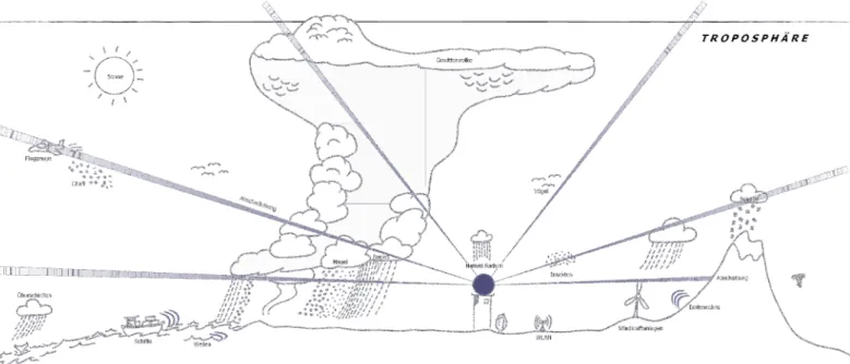
Figure 2.3:Schematic diagram of various sources of spurious echoes in weather radar data. Reprinted from Deutscher Wetterdienst (Wetter und Klima aus einer Hand), radar meteorology, radar data quality control.
Available from:https://www.dwd.de/EN/research/weatherforecasting/ met applications/radar data applications/radar data quality control node.html
2.2.2.2 Attenuation
Attenuation of EM waves by atmospheric gases is negligible. At wavelengths greater than 3 cm, the specific attenuation caused by atmospheric gases is less than 0.008 dB km−1
[Collier, 1996]. Note, most meteorological radars operate at a wavelength between 3 cm and 10 cm. Attenuation by clouds, cloud droplets or ice crystal clouds is more significant, but unlikely to be an issue. The attenuation by raindrops is much stronger and may result in significant underestimation of the strength and area of the precipitation, if left uncorrected, which can result in erroneous estimation of the damage potential. An example of the effect of rainfall-induced attenuation on radar measurement is illustrated in Fig. 2.4.
Figure 2.4:(a) Modification of the profile of a shower 20 km in width in which the intensity R of the precipitation varies by 10 mm h−1km−1. Rmis the minimum detectable
intensity. (b) Modification of the profile of a shower 20 km in width in which the intensity R of the precipitation varies by 5 mm h−1 km−1. Rm is the minimum
detectable intensity. (after [Treussart, 1968] and [Clift, 1985])
The phenomenon of EM wave attenuated by raindrops is due to the microphysical prop-erties of the intervening rainfall: the scattering cross sections, σb, σs and σa, where the subscripts stand for “backscatter”, “scatter” and “absorb” respectively, are defined by the
shape, size and temperature of individual raindrops. Among the transmitted power Pt, some (Pt×Pσs) is scattered and some (Pt×Pσa) is absorbed. Only a very small portion is backscattered to the radar antenna (Pt×Pσb). The scattering and absorption processes are subsumed as attenuation (dB) or specific attenuation (dB km−1
), while the backscattered signal is related to radar reflectivity factorZ (e.g. [Doviak and Zrni´c, 1993]; [Kr¨amer and Verworn, 2008]).
Similar as most rainfall-related variables, especially for radar reflectivityZand precipitation rate R, empirical power law is used to describe the relation between Z (mm6 m−3
) and the specific attenuation A (dB km−1
) [Gunn and East, 1954], and the relation between R (mm h−1
) and A [Hitschfeld and Bordan, 1954]:
A=aRb (2.4)
A=cZd (2.5)
where a, b, c and d are empirical parameters. Hitschfeld and Bordan [1954] were one of the first to investigate forward gate-by-gate procedures, used to correct for attenuation by the intervening rainfall. Path-integrated attenuation (PIA) is then obtained by accumulat-ing specific attenuation over the entire propagation path. Usaccumulat-ing equ (2.5), PIA of gate i is expressed by PIAi=c Zi+ i−1 X j=0 cZjd d ·2∆r (2.6)
where∆r is the gate length. The original reflectivityZiin dB of gate i is then corrected by adding the corresponding PIAi(dB)
Zcorr,i=Zi+PIAi (2.7)
The unconstrained PIA correction method has been widely criticized for its instability (e.g. Hitschfeld and Bordan themselves, [Hildebrand, 1978]; [Pfaff, 2013] and [Jacobi and Heis-termann, 2016]): small errors can grow exponentially over the propagation path, leading to errors much larger than if the data have not been corrected at all.
Due to the instability of the unconstrained PIA correction, modified versions of the method have been developed. Kr¨amer and Verworn [2008] proposed a scheme to stabilize the un-strained PIA method by fixing the exponent din equ (2.5), and the linear parameter c is then successively reduced for continuous beam sectors until the stability is achieved. The criterion to detect instability is when the attenuation-corrected reflectivityZcorr of any gate exceeds a maximum value ofZcorr,max= 59 dBZ, which is kind of arbitrary but legitimate from an operational point of view [Jacobi and Heistermann, 2016]. The 59 dBZ threshold is somehow supported by numerical experiments conducted by Islam [2008], who found the attenuation correction schemes become unstable when true reflectivity exceeds 60 dB.
Jacobi and Heistermann [2016] enhance the scheme proposed by Kr¨amer by introducing a second constraint, the upper limit of PIA is set to PIAmax= 20 dB as an additional criterion to detect instability, which is in agreement with PIA observations between radar and mountain reference targets at a distance of 120 km [Bouilloud et al., 2009]. The superiority of this approach compared to the one proposed by Harrison et al. [2000] is that PIA is not truncated at PIAmax, but reduced by decreasing the linear coefficient of the A-Z relation, factorc in equ (2.5), iteratively until they fall below PIAmax, in the same way as for the reflectivity limitZcorr,max. The instability is identified when PIA of any gate exceeding PIAmaxor if the correctedZ exceedingZcorr,max. The significant source of instability is removed at the cost of losing the ability to correct for extreme losses of the radar signal.
2.2.2.3 Anomalous Propagation
Due to the inherent variability of the atmosphere, the propagation conditions may dif-fer, sometimes significantly, from those considered “standard”, resulting in anomalous propagation condition (sometimes abbreviated asanapropor AP). A standard propagation condition means when a radio wave propagates through the air with the temperature that declines at a standard rate with the height in the troposphere, i.e. the temperature lapse rate. Under standard or normal propagation condition, the radar beam bends downward with a radius of curvature greater than that of the Earth’s surface (around 5/4 of the Earth’s radius of curvature). Consequently, the net effect is an increase of the height of the beam center as the distance from the radar site increases.
Figure 2.5:Occurrence principle of anomalous propagation echo. Anomalous Propagation Echo Classification of Imbalanced Radar Data with Support Vector Machine -Scientific Figure on ResearchGate. Available from:https://www.researchgate.net/ Occurrence-principle-of-anomalous-propagation-echo fig10 293482981[accessed 31 May, 2018]
less than the standard, and therefore radar is measuring something higher in the atmo-sphere. In contrast, super-refraction occurs when the radar beam bends more towards the Earth’s surface than the standard. Ducting, as an extreme case of super-refraction, occurs when the radius of curvature of the beam is smaller than that of the Earth’s surface, trap-ping the propagation pathway between a specific atmospheric layer and the Earth’s surface. The height of the beam center h is a function of the range r. The relationship is give by (e.g. [Doviak and Zrni´c, 1993]; [Bech et al., 2012])
h=pr2+ (k
eR)2+ 2rkeRsinθ−keR+H0 (2.8)
where,R is the Earth’s radius;ke is the ratio of R to the equivalent Earth’s radius; θis the elevation angle of the antenna andH0 is the antenna height. The propagation condition is
reflected in the value ofke, which can be formulated in terms of the refractivity gradient as
ke=
1
1 +R·dN dh
(2.9)
where,dN/dhis the vertical refractivity gradient (VRG). Usually, the atmosphere propaga-tion condipropaga-tion is characterized by the VRG of the air in the first kilometer above the ground level.
However, except for VRG, the angle of incidence and the frequency of the EM wave also play a role [ITU, 2003]. For weather radar application, if the VRG of the air in the first kilometer is around -39 N units km−1
, then standard propagation is considered for any angle of incidence [Doviak and Zrni´c, 1993]. From an operational point of view, normal propagation condition is assumed when the VRG is within the interval (-79, 0] N unitskm−1
. An increase in VRG bends the radar beam more slowly than normal (sub-refraction); while, a decrease in VRG bends the beam faster than normal (super-refraction), with a typical VRG value within the interval (-157, -79] N unitskm−1
, and ducting is induced when the VRG is lower than -157 N unitskm−1
[Bech et al., 2012].
Note, anaprop literally means anomalous propagation, including both the cases of sub- and super-refraction. However, anaprop echoes are only associated with super refraction and ducting. The occurrence of anaprop echoes is particularly negative for QPE by weather radar, and therefore should be removed. The occurrence of super-refraction and ducting is usually associated with temperature inversions of sharp water vapor vertical gradients. During cloudless nights, radiation cooling over land favors the formation of ducts which disappear as soon as the sun heats the ground, because of the destroying of the temperature inversion [Bech et al., 2012]. This process may be sometimes observed in the daily evolution of clutter echoes (e.g. [Moszkowicz et al., 1994], etc). There are several rules for the detec-tion of anaprop echoes, from which Lee et al. [2016] list four representative rules that are applicable in actual cases.
2.2.2.4 Uncertainty in Z-R relationship
Z-R relationship is used to convert radar reflectivity factor Z to precipitation intensity R. The uncertainty of Z-R relationship is considered as a massive source of uncertainty in quantita-tive precipitation estimation of weather radar. Z-R relationship varies with different rainfall regimes and geographic locations. However, even for the same rainfall regime and at the same geographical location, Z-R relation is still variable, as a function of time and space. The radar reflectivity factor Z (mm6/m3) of precipitation is dependent on the drop size dis-tribution of the hydrometeors in the radar sampling volume. The relation can be expressed by (e.g. [Battan, 1973]; [Uijlenhoet, 2001])
Z =
Z ∞
0
D6·Nv(D)dD (2.10)
whereNv(D)dDrepresents the mean number of raindrops with equivalent spherical diam-eters betweenDand D + dD (mm) per unit volume of air. Nv(D) is the so-called raindrop size distribution with the unitmm−1
m−3
.
Suppose raindrops precipitate without the influence of wind turbulence, no obvious updraft or downdraft and no interaction in between individual raindrops, then precipitation inten-sity R (mm/h) can be related to raindrop size distribution according to (e.g. [Uijlenhoet, 2001], etc)
R= 6π×10−4
Z ∞
0
D3·v(D)·Nv(D)dD (2.11) where v(D) represents terminal fall speed of droplets with the unit m/s. It is a function of the equivalent spherical raindrop diameterD(mm). v(D) is most widely depicted by a power law relationship
v(D) =cDγ (2.12)
Atlas and Ulbrich [1977] demonstrated the parameter values ofc = 3.778andγ = 0.67 in equ (2.12) provide a close fit to the data of Gunn and Kinzer [1949] in the range0.5 ≤D≤
5.0mm (the diameter interval contributing most to rain rate). As suggested by Uijlenhoet [2001], the exact values ofcandγ are not that important, yet what matters is the power law form ofv(D), which is consistent with the series of power law relationships of the rainfall-related variables, notably forZandR.
The comparison of equ (2.10) and equ (2.11) shows that radar reflectivity and precipita-tion rate are proporprecipita-tional to6thand approximately3.7thmoments of the raindrop diameter, respectively. Radar reflectivity is much more sensitive towards raindrop diameter than pre-cipitation rate. As a result, there exists no mathematical function linking Z and R. It is, therefore, essential to determine or estimate the raindrop size distribution, as it is the com-mon part of equ (2.10) and (2.11). Overwhelming empirical evidences (e.g. [Battan, 1973]; [Uijlenhoet, 2001]) have shown Z-R relation generally follows power laws of the form:
Z =aRb (2.13)
where a and b are coefficients depending on raindrop size distribution, rainfall regime and geographical location (e.g. [Lee and Zawadzki, 2005]; [Steiner et al., 2004]; [Hazenberg et al., 2011]).
Battan [1973] presents a summary of 69 Z-R relationships from numerous studies on differ-ent precipitation types and climate zones. There is appreciable variability in the coefficidiffer-ents of these Z-R relationships, e.g. the omnipresent Marshall-Palmer relationshipZ = 200R1.6
for stratiform rain [Marshall et al., 1955]; Z = 500R1.5 [Joss et al., 1970] or Z = 485R1.37 [Jones, 1956] for thunderstorm rain;Z = 140R1.5for drizzle [Joss et al., 1970], etc. Although
the DSDs obtained by electromechanical disdrometers or optical spectrometers can be used for procuring the Z-R relationships, these DSD measurements are not available in many parts of the world (e.g. [Hasan et al., 2014], etc).
As for the statement “Z-R relationship is a function of time and space”, which is made at the beginning of the section, the first term “Z-R relationship as a function of time” is relatively easy to understand. As different DSDs are expected at different stages of a storm, especially for convective events where the change in DSD is more rapid and intense, different Z-R relationships are therefore expected over the time.
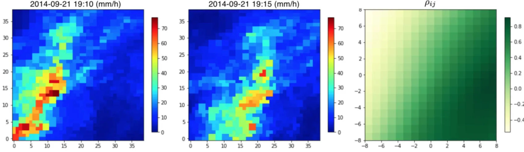
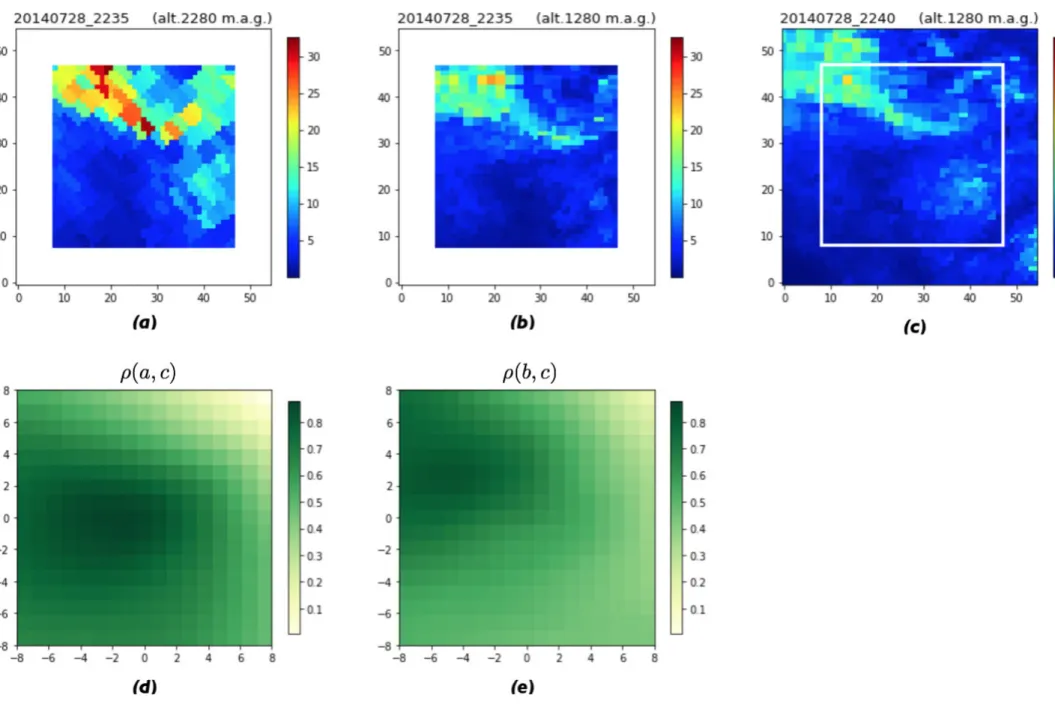
Figure 2.6:Synchronous maps of precipitation rate measured at 2280 m (left) and 1280 m (right) above the ground surface. Note, the time instant, unit as well as the data source (fbg for Radar Feldberd; tur for Radar T ¨urkheim) of the instantaneous map is labelled in the figure title and the resolution is 500 m×500 m.
In the chapter of introduction, the statement “Z-R relationship is a function of time and space” has been proved indirectly by the variability of DSD with time and height. In this
section, the second term “Z-R relationship as a function of height” is directly proved by the following two examples.
Fig. 2.6 shows two instantaneous maps of precipitation rate for the same domain and for the same instant provided by two weather radars. The only distinction between the left and the right is the measurement height: the left is measured 1000 m above the right, where the standard propagation of the radar beam is assumed. The Z-R relationship used in the con-version the reflectivity to rainfall rate isZ = 256R1.42, consistent with the parameterization
adopted by the German Weather Service (DWD), for the two radars in use are members of the 17 radar network operated by DWD.
Although the two measurements are for the same time and for the same area, the magni-tudes of precipitation intensity indicated by the two are fairly different: the left map shows an event with much stronger precipitation intensity than the right; while the opposite is true for the event shown by Fig. 2.7.
The two examples given in Fig. 2.6 and 2.7 reveal the variability of Z-R relationship along the vertical distance, which also implies the variability of radar reflectivity along the vertical distance. Hence to convert radar reflectivity measured at a certain altitude to precipitation intensity, Z-R relation at that altitude is required.
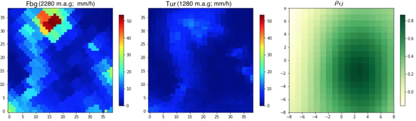
Figure 2.7:Synchronous maps of precipitation rate measured at 2280 m (left) and 1280 m (right) above the ground surface. Note, the time instant, unit as well as the data source (fbg for Radar Feldberd; tur for Radar T ¨urkheim) of the instantaneous map is labelled in the figure title and the resolution is 500 m×500 m.
The vertical variability of reflectivity is a massive source of error in terms of quantitative precipitation estimation using radar. It is also a factor limiting the effective range of radar as a rainfall sensor (e.g. [Joss et al., 1990]; [Fabry et al., 1992]). Because the more distant the
measurement level from the surface, the lower correlation of the measured reflectivity with the surface precipitation. The consequence of the vertical variability of reflectivity is more serious for weather radars operating in complex topographical settings, such as mountain regions (e.g. [Joss and Lee, 1995]; [Andrieu et al., 1997]), as the complex topography aggra-vates the variability.
A further comparison of the two maps in Fig. 2.6 and 2.7 shows that the two maps measured at different altitudes present very similar spatial patterns. In other words, if only the relative magnitudes are considered, the two maps are more or less the same.
Compared to the great variation of precipitation intensity (or other rainfall-related variables such as reflectivity or precipitation accumulation) along the vertical distance, the relative magnitudes, i.e. the spatial pattern, remains ralatively stable. It is therefore suggested in this study to use radar estimates of rainfall-related variable in the relative magnitudes, i.e. as a quantile map, to indicate the spatial pattern of the variable of interest at the ground surface.
2.2.2.5 Signal fluctuation
Radar echoes produced by precipitation fluctuate rapidly. The strength of signal varies from pulse to pulse. The type of target is subsumed as incoherent, as it is composed of many scatterers moving randomly; on contrast, solid targets, or scatterers moving in the same direction are subsumed as coherent [Collier, 1996].
What radar measures is the areal mean reflectivity, by calculating the mean of a number of independent samples. The samples for averaging purpose are collected gate by gate before the antenna is rotated to the next azimuthal angle. Keeping the radar antenna rotating at relatively low speed (e.g. 1 rev min−1
) helps in collecting more samples each gate, but at the cost of degrading the azimuthal resolution. Furthermore, the inherent variability of rain rate spatially and temporally, which on occasions can vary by a factor of 10 within a period of 10 min or within a distance of 2 km [Collier, 1996], prevents a reliable average reflectivity from being measured, particularly at far ranges, where the beam width is several kilometers’ wide.
2.2.2.6 Radial degradation of map quality
Radar data are originally in polar coordinates. As the distance of the target from the radar site increases, the resolution of radar imagery decreases. Take the C-band radar operated by DWD as an instance: one data set is composed of 360 radar rays (azimuthal resolution 1◦
), and each radar ray is subdivided into 128 gates with the gate length∆r = 1km. Thus, at Range 25 km, 75 km and 125 km, the corresponding beam widths are 0.44 km, 1.31 km and 2.18 km, respectively, according to
withLbeing the beam width,θbeing the azimuthal resolution andrbeing the range. Thus, the ratio of the resolutions of the three beam gates is 1 : 3 : 5.
More persuasive examples are given in Fig. 2.6 and 2.7. The weird looking of the left map is due to the futher distance of the domain from the radar site Feldberg. The relative position of the study domain in the radar polar coordinate is depicted in Fig. 2.8.
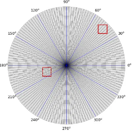
Figure 2.8:The relative positions of the study domain (represented by the red squares) in the radar polar coordinates: the square in the top right corner indicates the position of the study domain relative to Radar Feldberg, where the center of the domain is at 113 km’s range; the other square indicates the position of the study domain relative to Radar T ¨urkheim, where the center of the domain is at 45 km’s range.
However, the quality degradation of radar imagery discussed here is not only in terms of map resolution. In fact, many problems associated with quantitative precipitation estima-tion of radar are aggravated as the resoluestima-tion of radar imagery decreases or as the distance of the target from the radar site increases, for example, attenuation, signal fluctuation, vertical profile of reflectivity and non-uniform filling of the beam gate, etc.
2.2.3 General aspects of local radar data
The German Weather Service, abbreviated as DWD (Deutscher Wetterdienst), runs a net-work of 17 operational weather radars which are equipped with the latest dual polariza-tion Doppler technology. The 17 weather radars cover the whole Germany, providing many products for high resolution precipitation analysis and forecast. The scan strategy for the DWD’s radar network can be referred to under https://www.dwd.de/EN/ourservices/ radar products/radar products.html. The scanning cycle starts with the so-called precipitation scan, namely a near-surface scan during which the antenna follows the orography.
Fig. 2.9 shows the 17 radar network of DWD, with the study domain marked as a purple square. The study domain is covered by three radars. Among them, available data are from Radar T ¨urkheim and Radar Feldberg — see Table 2.2 for further details of the two radars. The 150 km coverage of the two radars are highlighted with two purple circles.
Weather radar takes snapshots of reflectivity distribution over large area from which the distribution of precipitation intensity is estimated. The snapshots of reflectivity are expressed as plan position indicators, or PPIs. There is a systematic change of PPIs in the observation height with range. As the domain is relatively small (a square with the side length of 19 km), the change in the elevation is neglected. The center of the domain is around 45 km from Radar T ¨urkheim and around 113 km from Radar Feldberg. With the elevation angle as low as possible to avoid ground echoes, according to equ (2.8), the measurement heights of Radar T ¨urkheim and Radar Feldberg for the study domain are respectively 1280 m and 2280 m above the ground (m. a. g.) under the normal propagation condition.
Table 2.2:Specification of Radar T ¨urkheim and Radar Feldberg
Item Specification Location T ¨urkheim 9.783◦ W, 48.585◦ N, 767.62 m.a.s.l. Location Feldberg 8.004◦ W, 47.874◦ N, 1516.10 m.a.s.l. Measured variables Radar reflectivity in dBZ, radio velocity Radar frequency 5.6 GHz
Elevation angle 0.5 – 1.8◦
(follow orography) Reflectivity quantization -32.5 up to 95.0 dBZ with 0.5 dBZ
increment Spatial resolution 1◦
×1 km (azimuth, range)
Range 128 km
Figure 2.9:Radar network of DWD, where the blue dot denotes each radar site and the blue circle indicates the radar coverage of 150 km range. The study domain is marked as a purple square with the side length of 19 km. The coverages of Radar T ¨urkheim and Radar Feldberg are highlighted with two purple circles. Reprinted from Deutscher Wetterdienst (Wetter und Klima aus einer Hand), weather fore-casting, numerical modeling. https://www.dwd.de/EN/research/weatherforecasting/ num modelling/bilder/02 datenassimilation abb09 en.html
The German Weather Service uses the DX file format to encode local radar sweeps. Raw, unprocessed DX products are in polar coordinates with the unit dBZ. The processing chain of DX products in this study is composed of (arranged in order): clutter removal, attenuation correction, conversion of reflectivity to precipitation rate, rainfall accumulation, re-projection from polar coordinates to Cartesian grid and clip the square data for the study domain. Some complementary descriptions about the processing chain are listed below.
• For clutter removal, despite the application of a Doppler filter at the signal proces-sor, the radar data still contains residual clutter (dynamic clutter), which can become considerable source of instability for the subsequent attenuation correction procedure [Kr¨amer and Verworn, 2008]. Therefore, the residual clutter is filtered out by the scheme proposed by Gabella and Notarpietro [2002], based on a texture filter that de-tects strong reflectivity gradients.
• For attenuation correction, the constrained gate-by-gate attenuation correction scheme is applied ([Kr¨amer and Verworn, 2008]; [Jacobi and Heistermann, 2016]).
• For the conversion of reflectivity to precipitation rate, the Z-R relation is parameterized asZ = 256R1.42, consistent with the parameterization adopted by DWD.
• For the re-projection from polar coordinates (Resolution: 1◦
×1 km) to Cartesian grid (Resolution: 500 m×500 m), nearest neighbor method is applied, no interpolation is conducted.
All the radar data processing steps in this study are operated under the environment of
wradlib, an open source library for weather radar data processing. wradlib is written in the free programming language Python, and a tutorial on a typical workflow for radar-based rainfall estimation is available underhttp://docs.wradlib.org/en/latest/notebooks/basics/wradlib workflow.html.