Date of publication xxxx 00, 0000, date of current version xxxx 00, 0000. Digital Object Identifier 10.1109/ACCESS.2017.DOI
Cell Fault Management using Machine
Learning Techniques
DAVID MULVEY1, CHUAN HENG FOH1(SENIOR MEMBER, IEEE), MUHAMMAD ALI IMRAN2 (SENIOR MEMBER, IEEE), AND RAHIM TAFAZOLLI1(Senior Member, IEEE).
15G Innovation Center, University of Surrey, Guildford, UK 2School of Engineering, University of Glasgow, Glasgow, UK
Corresponding author: David Mulvey (e-mail: d.mulvey@surrey,ac.uk).
This research was partly funded by the EPSRC Global Challenges Research Fund (the DARE project) EP/P028764/1.
ABSTRACT This paper surveys the literature relating to the application of machine learning to fault management in cellular networks from an operational perspective. We summarise the main issues as 5G networks evolve, and their implications for fault management. We describe the relevant machine learning techniques through to deep learning, and survey the progress which has been made in their application, based on the building blocks of a typical fault management system. We review recent work to develop the abilities of deep learning systems to explain and justify their recommendations to network operators. We discuss forthcoming changes in network architecture which are likely to impact fault management and offer a vision of how fault management systems can exploit deep learning in the future. We identify a series of research topics for further study in order to achieve this.
INDEX TERMS Cellular networks, self healing, cell outage, cell degradation, fault diagnosis, deep learning, explainable AI
I. INTRODUCTION
T
HE pressure to achieve greater data rates from limited radio spectrum resources is driving changes in cellular network architecture as 5G evolves. A decentralised Radio Access Network (RAN) architecture has emerged where groups of small, densely deployed cells are associated with a single macrocell, with signalling transmission retained by the macrocell but user traffic largely devolved to the small cells [1], [2] and [3]. In addition, optional interfaces between baseband and RF processing have been defined, enabling the potential virtualisation of some RAN functions.In the new RAN architecture, Coordinated Multipoint (CoMP) transmission techniques , based on Multi User Mul-tiple Input MulMul-tiple Output (MU-MIMO) configurations, are used to maximise radio throughput [4]. Small cells in urban settings use three-dimensional MIMO, with planar array antennas containing significant numbers of antenna elements [5].
At the same time, other work has been going on to ad-dress the topic of energy efficiency, given that the energy consumption of cellular networks is typically dominated by that of the base stations. This will require complex strategies to adjust cell coverage and turn base stations off and on again
depending on traffic levels, without disruption to users [6]. These additional capabilities included in the new RAN architecture will require it to have many more configurable parameters than previous generations [7], [8] and [9], whose settings may vary according to local conditions. This will mean that the classic strategy of building a set of rules to handle faults is likely to begin to break down as the ruleset becomes too large, complex and difficult to maintain. In this situation there is an opportunity to exploit the benefits of machine learning (ML) based techniques, in particular deep learning, which do not require an explicit causal model, such as a ruleset, in order to be effective.
We define fault management as the set of tasks required to detect cell faults and then identify and implement corrective actions to restore full operation. We also include any activi-ties required to determine the root cause of a fault, in order to take steps to prevent a recurrence. We exclude administrative tasks for tracking faults and organising remedial work from the scope of this definition.
These tasks may be carried out by the network manage-ment team or may be at least partly automated. In the latter case, such features are being specified and developed for mobile networks under the banner of the Self Organising
Network (SON). The EU SOCRATES project has defined use cases for the SON, leading to subsequent formalisation in the 3GPP standards [10], [11], [12] and [13]. The main threads within the SON are self configuration, self optimi-sation and self healing, all of which have some relevance to fault management, especially self healing. The top level SON standard [11] provides for both partial and full automation. In the former case, referred to as open loop SON, operator con-firmation is required before control actions are implemented. In the latter case, known as closed loop SON, the system is fully automatic requiring no operator intervention.
Three approaches to fault management have been de-scribed in the literature: rule based systems, algorithmic approaches and most recently machine learning techniques.
Rule based systems have the key advantage that presenting their chain of reasoning to a user is relatively straightforward, but have the major disadvantage that they require the use of network domain expertise to set up and maintain the ruleset.
Algorithmic approaches can be very effective but lack the transparency of rule based systems and are typically limited to a narrow problem area, requiring the use of diverse algorithms to cover the complete fault management problem space, each requiring input from both network domain ex-perts and algorithm specialists to set it up and maintain it.
Machine learning (ML) approaches, by contrast, can offer several benefits. At the root cause analysis stage, ML tech-niques can be used to trawl through very large volumes of fault data to suggest possible symptom-cause linkages which an expert can then review.
For real time fault management, ML techniques [14], [15], [16] and [17] have the advantage that they can be trained from fault data with limited domain expert input, and can then be retrained semi-automatically as the network changes. Unlike algorithmic methods, ML techniques are typically able to cover a broad range of problem areas, reducing the need for input from staff with knowledge of specialist algorithms. Deep neural networks, a recent development in ML [18], [19] and [20], are able to process very large and complex input data sets without the need for much of the dedicated handcrafted preprocessing code required by rule based and algorithmic techniques.
An issue has emerged, however, in that the most promising recent ML techniques such as deep learning, unlike earlier approaches such as Bayesian networks, do not attempt to build a casual model of the network and instead exploit cor-relations between data items reported by the network. Hence these techniques take no account of underlying engineering principles in arriving at their decisions. A key challenge, therefore, will be to find a way to give such systems the ability to explain and justify their recommendations.
The main contributions of this paper are as follows: • we review and discuss the application of ML techniques
to cell fault management from an operational perspec-tive, considering fault management as a cooperative activity between the network management team and a range of electronic systems
• we propose a revised fault management lifecycle based on emerging industry practice
• we cover root cause analysis in addition to the classic self healing tasks (detection, diagnosis and compensa-tion) covered by previous surveys
• we cover deep learning as well as earlier ML approaches and their non-ML predecessors
• we review the approaches which can be taken to enable an ML subsystem to explain its recommendations • we propose a standard set of metrics against which to
evaluate fault management systems
This paper is organised as follows. After reviewing related work, we propose a revised lifecycle for fault management aligned with the most recent operational practice, and discuss the issues in capturing the data required to support the pro-cesses within this framework. We discuss pre-ML techniques and their limitations before moving on to introduce the key ML approaches. We then survey the application of ML techniques to fault management in mobile networks, based on the key building blocks of a typical fault management system. After this, we consider the impact of recent changes in network architecture and identify the gaps between the key attributes of a future fault management system and the cur-rent state of the art. Finally we list areas for future research to close these gaps.
II. RELATED WORK
Previous surveys in fault management focus on SONs as fully automated systems, with some discussion of how ML approaches can be applied to self healing. In this paper, we also include system-operator interaction, over the full range of fault management activities as defined above including root cause analysis, taking into account the most recent developments in deep neural networks.
Aliu et al. [21] cover all aspects of self organisation in cellular networks, with particular emphasis on self optimi-sation; the authors note that relatively little work has been reported on self healing in relation to the other SON func-tions. The paper gives an overview of cell outage detection and compensation and provides a useful taxonomy of ma-chine learning techniques applicable to SONs generally. This includes neural networks but coverage of these is restricted to self organising maps. Among other future research topics the paper highlights the need for work to ensure satisfactory interworking between self healing and energy saving cell hibernation schemes.
Klaine et al. [22] also survey machine learning applied to self organising networks, under the headings of self op-timisation, self configuration and self healing. Self healing is defined to cover fault detection, fault classification and cell outage management (detection through to fault compensa-tion). A wide range of earlier machine learning techniques is covered and discussed. There is one reference covering neu-ral networks applied to self healing, which uses a feedforward network.
Asghar et al. [23], by contrast, focus on self healing and survey a broad range of techniques which have been applied to detection, diagnosis and compensation for cell outages. These include ML approaches, but discussion of the more recent techniques including NNs is limited. They raise a number of very interesting points on future challenges, mainly recommending algorithmic approaches as the way forward rather than the application of ML techniques.
All the above papers focus on closed loop rather than open loop SON. Self healing is taken to be an automatic subsystem which is able to run autonomously, and so the capabilities required to interact with a human user are not covered.
In the current paper, however, we consider fault ment as a cooperative activity between the network manage-ment team and automated technologies designed to alleviate their workload. Hence we cover both open and closed loop SON, as well as support for expert investigations into under-lying issues. We consider more recent techniques which are just beginning to be applied to fault management, such as deep neural networks and deep reinforcement learning. We also include the analysis of successful operator actions as an alternative perspective to fault data analysis. As part of this, we also assess the person to machine interaction issues that will need to be addressed to enable network management teams to work effectively with these new tools.
III. FAULT MANAGEMENT FRAMEWORK A. DEFINITIONS
Network Fault(s) Corrected
Detection Diagnosis Compensation Recovery
Identify compensation and recovery actions Raise alert if fault present Re-establish normal service as far as practicable Restore network to full normal service
FIGURE 1. Self Healing Lifecycle
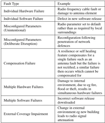
For the purposes of this paper, we consider a fault to be a state of the radio network or one or more of its elements which causes the network to fail to meet its service specifica-tion. For the RAN we can define the service being provided as the connectivity from the core network across the RAN to the end user’s mobile device. The types of faults we consider, with typical examples, are given in Table 1.
A set of symptoms indicating a fault, observed at the service level and from other evidence within the network, may be due to one or more underlyingcauses, in the context of a set of networkconditions.
Causes of faults may include hardware failures, software defects, design flaws, misconfigured parameters, incorrect
TABLE 1. Typical Examples of Cell Faults
Fault Type Example
Individual Hardware Failure Radio frequency cable fault ordamage to antenna element Individual Software Failure Defect in new software release Misconfigured Parameters
(Unintentional)
Radio parameter set to default rather than as required by local surroundings Misconfigured Parameters (Deliberate Disruption) Reconfiguration following penetration of network defences Compensation Failure
A resilience or self healing feature compensates for a single failure such as an antenna fault but the failure is not rectified; a similar failure then occurs which cannot be compensated for
Multiple Hardware Failures
Damage to internal environment, due to eg fire, flood or theft, results in simultaneous hardware failures Multiple Software Failures Incorrect software release
downloaded
External Coverage Impairment
Change in external environment eg new building leads to radio signal attenuation
actions by the network operations team and unauthorised external interventions (cyber attacks) which have succeeded in penetrating the network’s security defences.
Fault symptoms may have several possible causes; an unacceptably high dropped call rate, for example, could be due to factors such as a hardware failure, an incorrect setting of a parameter e.g. antenna tilt, or even a change in the local surroundings which causes a reduction in radio signal strength.
Different types of faults may need to be handled differ-ently. Specific unintentional misconfigurations, for example, can be fixed with the likelihood that the issue will remain resolved. Deliberate disruptions, however, may recur unless steps are taken to prevent external attack or mitigate its effects. Even in the unintentional case it may be necessary to prevent future failures by measures such as retraining or additional checks. We discuss the issue of analysing the root cause of a fault and devising preventive measures in more detail below.
At the compensation stage a failure is compensated for by a self healing or system resilience feature (such as an automatic switch from main to standby) but the failure is typically not yet rectified, so that it becomes adormant fault. In this paper we consider all the fault types listed in Table 1. We assume that there is a separate operational process in place (outside the scope of this paper) for dormant faults to be logged and managed, which reports such faults to the fault management system so that they can be considered together with the presenting fault symptoms.
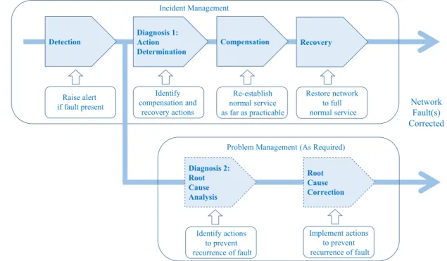
Incident Management
Problem Management (As Required) Diagnosis 1:
Action Determination
Detection Compensation Recovery
Diagnosis 2: Root Cause Analysis Root Cause Correction Re-establish normal service as far as practicable Raise alert if fault present Restore network to full normal service Identify actions to prevent recurrence of fault Implement actions to prevent recurrence of fault Identify compensation and recovery actions Network Fault(s) Corrected
FIGURE 2. Fault Management Lifecycle
B. FAULT LIFECYCLE
Many of the studies we reference in this paper are based on the lifecycle for self healing systems (see Fig. 9), which fo-cuses on the immediate activities required to get the network back into operation following a fault [24]. Recent operational fault management practice, however, has been based on a slightly different lifecycle which has a wider scope. We propose a revised and extended lifecycle, which is intended to reconcile these two approaches (see Fig. 2).
The self healing systems lifecycle described in [24] con-sists of a single phase of fault handling with four stages: de-tection, diagnosis (also known as localisation), compensation (also known as mitigation) and recovery. On completion of the fault recovery stage the self healing process is complete, in that the system has now been restored to full normal operation.
The ISO20000 fault management standard, however, which is coming to be accepted in industry, considers fault management as having two phases:
1. Incident Management, where the primary objective is to restore service following detection of a fault.
2. Problem Management, where the objective is to in-vestigate in depth a single complex fault, or a number of apparently related faults, in order to devise suitable corrective action.
It can be seen that the lifecycle for self healing maps neatly onto that for incident management. Problem management, on the other hand, requires the addition of a second phase consisting of two stages which we may call root cause analysis and root cause corrective action.
At present, diagnosis and root cause analysis are not
always distinguished clearly in the literature, although the ML approaches to the two areas may well be different. To clarify this, we propose to divide the activity currently referred to as fault diagnosis into two separate parts, with different functions, to allow the relevant ML techniques to be considered separately.
We may call the first part Action Determination, repre-senting the diagnostic activities within Incident Management. Here the goal is simply to determine which compensation action to take given the symptoms. The second part can then be mapped on to the Root Cause Analysis stage of Problem Management. This part is potentially more demanding in that it is now necessary to analyse the fault in sufficient detail to be able to devise suitable corrective action to prevent a recurrence.
IV. FAULT MANAGEMENT DATA
In this section we consider the data required to implement the fault management framework outlined in the previous section, how this can be collected and what issues can arise. In later sections we will then go on to discuss how these issues can be addressed.
A. DATA SOURCES
In order to carry out fault detection and diagnosis, the system needs access to live data and to historic network data, cap-tured both during normal operation and also when a variety of faults are present. Key sources of data include alarms, other events, Key Performance Indicators (KPIs), radio coverage reports and network configuration data.
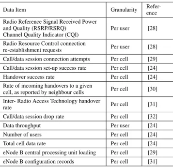
TABLE 2. Examples of Key Data for Cell Fault Management
Data Item Granularity
Refer-ence Radio Reference Signal Received Power
and Quality (RSRP/RSRQ) Channel Quality Indicator (CQI)
Per user [28] Radio Resource Control connection
re-establishment requests Per user [28] Call/data session connection attempts Per cell [29] Call/data session set-up success rate Per cell [24] Handover success rate Per cell [24] Rate of incoming handovers to a given
cell, as reported by neighbour cells Per cell [30] Inter- Radio Access Technology handover
rate Per cell [31]
Call/data session drop rate Per cell [32]
Data throughput Per user [24]
Number of users Per cell [24]
Total cell data rate Per cell [24] eNode B central processing unit loading Per cell [29] eNode B configuration records Per cell [31]
and managing the datasets relevant to SONs, including self healing systems, which can be drawn upon to consider the dataset required for fault management. The set of standard KPIs for cellular networks defined in [26] also forms a useful starting point; however Szilagyi et al.highlight that additional, lower level, data is likely to be required for cell fault detection and diagnosis [27]. Typical examples of key data referred to in fault management studies are given in Table 2.
B. DATA COLLECTION
To be useful for fault management, all data needs to be logged with a timestamp and also a spatial reference, which should at least identify the cell ID. For radio measurements it is highly desirable that the spatial reference should also include the location of the mobile at the time the measurements were made [33]. Relevant aspects of the network configuration at the time of logging also need to be recorded [24].
The 3GPP standards specify a mechanism for automatic cell data collection known as the cell trace facility, which reports the data to a central trace collection entity [34], [35] and [36]. This facility provides the ability to selectively enable and disable different trace functions in different areas of the network. For example, the Radio Link Failure (RLF) function can be used to instruct a specific eNodeB to collect and report UE radio link failure messages.
The traditional method of obtaining radio coverage data is drive testing, which is, however, increasingly expensive. Consequently 3GPP set up the Minimise Drive Testing (MDT) initiative, and as a result of this work have now incor-porated MDT data collection into the cell trace mechanism. This function collects UE measurements of radio KPIs such as RSRP and RSRQ, either regularly or in response to certain
network events, and passes them to the cell trace facility for logging [37], [38] and [39].
At around the same time, mobile devices evolved to in-clude a GPS location tracker, which was able to provide location data to a higher accuracy and resolution than previ-ously possible. As well as significantly enhancing the quality of radio reporting data for fault management, it has been recognised that this can be used to improve many aspects of radio network performance including interference manage-ment, scheduling and handover decisions [40], [41].
C. DATA QUALITY ISSUES
Typical examples of low level quality issues which can arise are noise, missing data and irrelevant data. Radio data, for example, can be subject to unwanted disturbances due to shadowing and fast fading of the signal. Equipment status reports, on the other hand, may consist entirely of clean data but some reports may be lost in transmission. Even with the level of control provided by the cell trace facility, reports may include data which is not relevant to the problem being addressed. Alternatively the volume of low level data items may be too high for efficient processing, or the data may only be available in a continuous stream whereas the ML technique may require data to be submitted in batches.
At a higher level, it may not be straightforward even to detect that a fault has occurred, given the available data. This is the case with the so-called “sleeping cell" problem [42].
This scenario arises because some faults, such as RF cable failures, cannot reported to the network management centre although they may cause a radio outage. If such a fault occurs, the user service may be significantly impacted without the network management centre being aware of the problem.
In some situations, individual data items may each be weakly correlated with the occurrence of a given fault or one of its causes, but for certain combinations of data items the correlation may increase significantly. Another possibility is that some of the data items may be correlated with each other, so that the dataset contains a level of redundancy which could lead to inefficient processing.
Alternatively far too much potentially relevant data may be generated, such as when a single low level fault, e.g a power supply failure, causes multiple alarm messages to be triggered, making it difficult for the network operators to determine the underlying cause.
In the next three sections we look at how all these issues can be overcome, either by suitable pre-processing of the data or by the fault management techniques themselves. Before this, we explain why ML approaches emerged by considering pre-ML techniques and their limitations.
V. PRE-ML FAULT MANAGEMENT SYSTEMS
Pre-ML fault management techniques can be divided into two principal categories: logic based and algorithmic.
Logic based approaches use a set of rules to explicitly encode knowledge about the relationships between fault
symptoms and causes. Algorithmic techniques, on the other hand, incorporate expert knowledge implicitly within the software implementing the algorithm. We discuss each of these approaches in turn and look at the limitations of both methods.
A. LOGIC BASED APPROACHES
In logic based approaches, the rules may be based on pred-icate logic (where predpred-icates are either true or false) or one of a number of developments of this to allow predicates to be associated with a probability rather than a binary truth value [43].
The earliest implementations were based on a hard coded program, with access to the rules embedded in the program at appropriate points. The rules themselves were encoded in a table or defined explicitly using a rule syntax. A development of this was the expert system, which separates out control into a separate entity, the inference engine, which is responsible for selection of which rules to activate [44]. In this architec-ture the rules are held in a data store known as the knowledge base.
A key application of logic-based systems is to address the multiple alarm issue described in Section IV above. This uses a technique called alarm correlation, in which low level alarms are filtered and aggregated based on a ruleset, to provide a more effective presentation of the network status to the operators [45].
A further refinement is the model based approach, which separates out the behaviour of each type of network element from the network topology, and models the expected normal behaviour of each element to enable this to be compared with the actual behaviour in order to determine whether a fault exists [46].
As a sophisticated example of this approach, Yan et al. developed a root cause analysis toolset called G-RCA [47]. This is designed for IP networks and includes a service dependency model incorporating topological relationships as well as dependencies between protocol layers. Candidate diagnosis rules are extracted from historic data using spatial and temporal “joining rules" specifying the allowable gap in time or distance in space between symptoms and potential causes. The resulting rules are verified by domain experts (the network operators) and then incorporated into a causality graph which controls the diagnosis of incoming symptoms.
B. ALGORITHMIC TECHNIQUES
The logic based approach is sufficiently generic to cover a wide variety of faults. Algorithmic techniques, on the other hand, are typically designed to address one very specific issue. An example of this is the problem of compensation for radio transmit/receive array failures, where Yeo et al. used a genetic algorithm to optimise radio performance of the failed array, and subsequently improved on this approach by using a particle swarm optimisation algorithm [48] and [49]. Closely related to this is the problem of compensation for cell outages, for which some recent examples of algorithmic
techniques again include particle swarm optimisation and also use of a proportional-fair utility algorithm [50] and [51].
C. LIMITATIONS
Logic based systems have proved effective in use but suffer from a number of serious limitations. Strict application of binary logic has been found to result in too many special conditions and so it has become necessary to group together various sets of symptoms and use probabilistic logic. Even so, rule bases can grow to the point where maintaining con-sistency becomes a major issue [43]. Given the complexity of 5G and the expected numbers of parameter settings, it may prove infeasible to use rule based systems at the level of detail required for effective diagnosis.
Expert input is required to set up and maintain the rule base and this can be scarce and expensive; the expert may not necessarily be able to articulate their knowledge so knowl-edge capture can be challenging [52]. Even the more recent systems with automated extraction of candidate diagnostic rules can require significant input from domain experts and software specialists to verify the logic initially and to main-tain it as changes are made to the network.
Logic based systems require the same pre-processing tech-niques to handle low level data issues as for ML systems (see Section VII below), and in addition may also require exten-sive domain and problem specific data conversion routines at the front end to turn complex analogue measurements, such as comparison against a profile, into simple predicates for processing by the ruleset.
Algorithmic approaches entail similar pre-processing overhead, together with significant expert input to code, set up and maintain the fault management subsystem. In addition such techniques are typically designed to solve one particular issue and do not generalise to other issues, which may lead to a large number of different low level software modules to be supported.
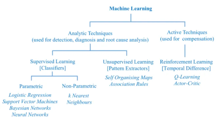
VI. OVERVIEW OF MACHINE LEARNING FOR CELL FAULT MANAGEMENT
By contrast with traditional logic based techniques, ML approaches can automate much of the work of setting up and maintaining the fault management system, so that expert input is only needed to validate the system rather than to specify all the details. Unlike algorithmic approaches, ML techniques can in many cases be used to handle a range of issues rather than being crafted to address one specific problem.
This section provides an overview of selected ML tech-niques which have been used in cell fault management stud-ies or have shown potential for cell fault management from their successful application in similar work. We also critically evaluate the advantages and disadvantages of ML approaches in relation to previous approaches.
For the purposes of this paper we use Murphy’s definition of ML: “we define machine learning as a set of methods that can automatically detect patterns in data, and then use the
Analytic Techniques
(used for detection, diagnosis and root cause analysis)
Active Techniques (used for compensation)
Supervised Learning [Classifiers] Unsupervised Learning [Pattern Extractors] Reinforcement Learning [Temporal Difference] Machine Learning Parametric Non-Parametric k Nearest Neighbours Logistic Regression
Support Vector Machines Bayesian Networks
Neural Networks
Self Organising Maps Association Rules
Q-Learning Actor-Critic
FIGURE 3. Taxonomy for ML Techniques in Cell Fault Management
uncovered patterns to predict future data, or to perform other kinds of decision-making under uncertainty" [53]. We can divide ML techniques applicable to fault management into two types. The first uses analytical techniques, where the sys-tem provides useful information derived from a raw data set [54], [53]. The second employs active techniques, where the system takes actions subject to a feedback and reward system [55]. To date, detection and diagnosis have been carried out using purely analytical approaches whereas active techniques have been exclusively applied to the compensation stage.
A taxonomy diagram for the principal ML techniques which have been used in cell fault management studies is given in Fig. 3.
A. ANALYTICAL TECHNIQUES
1) Introduction
All analytical ML techniques use two principal input data sets: training data made up of historical data, from which learning can take place, and active live data samples pro-cessed by the system when in operational use. In the ML world, the attributes of the input data are referred to as features; hence thedimensionalityof the data is the number of features.
We can consider the analytical techniques as having the following attributes, which are described in more detail be-low:
• output type (continuous, discrete)
• supervision mode (supervised, unsupervised) • training method (parametric, non parametric) • scope (global, local)
If the output type of an ML system is continuous, being used to predict some property derived from the input data set, the system is known as aregressionsystem. By contrast, systems in which the output type is discrete, so that each out-put represents a class to which each inout-put has been assigned, are referred to asclassificationsystems.
The supervision mode is dependent on the composition of the training dataset. Insupervised learningthe training data set includes values for the output data as well as the input data; these will be either predicted values in the regression case or class labels in the classification case. Inunsupervised
learning no predictions or labels are provided; the system uses input data only.
The training method used may beparametricornon para-metric. A parametric method fits a model to the training data during a training phase by adjusting the model parameters to minimise a suitable cost metric. The model is then used during a subsequent operational phase to predict from or classify live data. A non parametric method, on the other hand, uses the training data directly during the operational phase rather than learning a predictive or classification model beforehand.
The scope of either method may be global, in which case the algorithm takes as input the whole of the training dataset and any parameters are constant across the whole data range, orlocal, in which case the algorithm considers limited regions of the data space at a time and any parameters have local validity only, typically with a method of minimising discontinuities at the borders between the regions.
Methods may be based on purelylinearcalculation tech-niques, or may in addition includenon linearmathematical approaches. An important class of model based approaches which combines both of these is the neural network (NN). NNs consist of a set of nodes, each of which applies a specific linear weighting to each of its inputs and then may apply a non-linear transformation to compress the result. Nodes are typically organised in layers, providing input and output and also often including internal or hidden layers. Recent general advances in NNs have focused on so-called deep NNs , which for the purposes of this paper we may define as NNs with two or more hidden layers [56].
A good example of the NN approach is the feedforward NN (FFNN), typically used in cellular networks as a clas-sifier. This is trained by optimising the weights, using both the forward and the backward paths through the network, to minimise a “loss function" giving a measure of the difference between the labelled classification and that predicted by the NN. During the operational phase, classification then takes place using the forward path only.
An FFNN is unsuitable for processing input sequences as it can only consider a fixed set of inputs at a given time. This limitation would mean that an FFNN would be restricted to processing fixed length sequences and the number of input weights required would be the product of the number of features and the sequence length. To overcome this, the recurrent NN (RNN) feeds back the values of the states of each hidden layer and weights them to include in the calculations for the new state values for that layer for the next item in the sequence. This allows the weights to be shared between all items in the sequence and permits the processing of sequences of arbitrary length. As with the FFNN, the RNN is trained using labelled data.
A convolutional NN (CNN) by contrast, is designed to pro-cess two dimensional inputs, typically extracted from image data. As with an FFNN, a convolutional network consists of an input layer, an output layer and a number of hidden layers. The CNN, however, consists of two principal types of hidden
layer: the convolutional layer and the pooling layer.
The convolutional layer carries out a set of weighted convolution operations on small subsets of the layer’s inputs, using the same weights for each subset. The pooling layer, on the other hand, takes the outputs from the convolution layer and aggregates then across larger subsets of the data. This has the effect of making the results insensitive to particular aspects of the image such as the exact location or orientation of an item within the image. Repeating these processes over many hidden layers allows the CNN to learn its own features, such as lines or angles, which can become progressively more complex in the later hidden layers. Just as with the FFNN and the RNN, the CNN is trained using labelled data.
All the NNs described so far are typically used to predict the classification of data items, based on labelled training examples. The autoencoder, however, is designed to predict its own inputs. This can be useful when dealing with noisy inputs, when a so-called denoising autoencoder [57] can be used to recover a clean version of the inputs. The network consists of an encoder and a decoder, and is trained using a loss function providing a measure of the difference between the actual input and the autoencoder’s prediction of it. For more detail on recent developments in neural networks appli-cable to wireless networks see [18], [19] and [20].
At present, relatively little use of neural networks has been made in cell fault management, although an FFNN has been used for cell outage detection [58]. We discuss later on in this paper how deep NNs can be used in cell fault management and the challenges that will need to be overcome in order to achieve this.
2) Supervised Learning - Classifiers
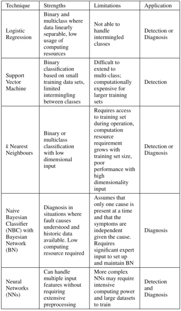
Detection and diagnosis techniques typically make use of classifiers based on supervised learning; binary classifiers are sufficient for detection where there are only two possibilities, faulty or not faulty, whereas for diagnosis, where there may be several possible causes, multiclass classifiers are required. A comparison of the major classifiers used in fault man-agement is given in Table 3. The simplest is logistic regres-sion, a parametric linear classifier, which finds a hyperplane to be used to separate the data, based on the minimum total squared distances from all the data points. It can be extended to permit non-linear boundaries by calculating new features which are polynomial or other functions of the original features.
The support vector machine (SVM) is also a parametric classifier but includes an internal non-linear transformation which allows it to handle non-linear boundaries. The SVM’s distinctive feature is that it sets the boundary by taking into account just the points close to where the boundary is expected to be, referred to in the literature as the support vectors. These points are identified in relation to a specified margin on either side of the boundary. A refinement is to set a budget for misclassification errors (points deliberately allowed to be on the wrong side of the boundary or in the margin). The position of the boundary is then adjusted by
TABLE 3. Principal ML Techniques 1: Classifiers
Technique Strengths Limitations Application
Logistic Regression Binary and multiclass where data linearly separable, low usage of computing resources Not able to handle intermingled classes Detection or Diagnosis Support Vector Machine Binary classification based on small training data sets, limited intermingling between classes Difficult to extend to multi-class; computationally expensive for larger training sets Detection kNearest Neighbours Binary or multiclass classification with low dimensional input Requires access to training set during operation, computation resource requirement grows with training set size, poor performance with high dimensionality input Detection or Diagnosis Naive Bayesian Classifier (NBC) with Bayesian Network (BN) Diagnosis in situations where fault causes understood and historic data available. Low computing resource required Assumes that only one cause is present at a time and that the symptoms are independent given the cause. Requires significant expert input to set up and maintain BN Diagnosis Neural Networks (NNs) Can handle multiple input features without requiring extensive preprocessing More complex NNs may require intensive computing power and large datasets to train
Detection and Diagnosis
an optimisation function to minimise the classification error subject to this budget.
The k nearest neighbours (kNN) method is a non-parametric approach. When used as a classifier,kNN requires training data to be gathered from normal and faulty operation, with the data labelled to distinguish between normal opera-tion and each type of fault. It then classifies each live data point by majority voting based on the labels of its knearest neighbours in the training set. A recently reported technique [59] is the Transductive Confidence Machine (TCM), which can be thought of as a variation of kNN which also uses a labelled training set. There is also a type ofkNN which can be used as anomaly detector. This method uses a training data set representing normal operation; for each live data point the system calculates a metric based on the distances from the knearest neighbours in the training dataset and compares it with a threshold in order to detect anomalies.
TABLE 4. Principal ML Techniques 2: Pattern Extractors
Technique Strengths Limitations Application
Self Organising Maps Mapping a high dimensional dataset onto a 1D or 2D discrete data set representing data clusters. Computing resource requirement depends on data set size, dimensionality and number of clusters. Additional cluster validation algorithms and expert input required. Diagnosis Association Rules (FP-Growth algorithm and modifi-cations) Extraction of associations (eg symptom-cause) from historic fault data. Unmodified algorithm requires frequent associations but modified version can work with rare associations (see Root Cause Analysis below).
Diagnosis
The naive Bayesian classifier (NBC) works with a Bayesian Network representing symptom-cause relationships derived from historic fault data. It uses Bayes’ theorem to rank the possible causes by probability given the symptoms. Expert input is required to set up the network but the cause probabilities can be estimated automatically if sufficient data is available.
An NN used as a classifier, irrespective of the number and type of the hidden layers, typically will have an output stage designed to estimate the probability of each input example being in each of the classes and use this to make a classification decision.
3) Unsupervised Learning - Pattern Extractors
All the above techniques depend on a training set with every data item labelled individually, which can require a large amount of expert input. As a result unsupervised learning techniques have been developed (see Table 4), which auto-matically extract a small number of patterns from large quan-tities of data. The candidate patterns can then be reviewed by experts, significantly reducing their workload in comparison with searching the data manually. Having done this the classifier can then classify the data by comparing it with the patterns. Although these approaches are typically somewhat computationally intensive during the training phase, none of them requires significant computing resource during the operational phase, as only the classifier needs to be run at this point.
One approach to pattern extraction is cluster analysis, which aims to group the data into similar types or clusters. An approach which has been used in fault diagnosis is self organising maps [60], which are a type of neural network
Action Environment State Reward Agent Value Function Calculate expected future reward Policy Select Action
FIGURE 4. Reinforcement Learning Architecture
TABLE 5. Principal ML Techniques 3: Reinforcement Learning Technique Strengths Limitations Application Temporal Difference (Q-learning) with Fuzzy Logic Model of underlying system (radio network) not required for optimisation Relatively slow to converge Compensation Temporal Difference (Actor-Critic) As above Slightly faster to converge than Q-Learning (see Compensation section below) Compensation
that projects a high dimensional training data space onto a very low dimensional (typically 1 or 2D) discrete data space representing a small number of clusters.
Another approach, which has been used in the root cause analysis of faults, is to use an association rule extractor algorithm [61] to scan network event logs and traces to automatically detect possible associations between a given set of symptoms and potential causes, together with measures of the strength of the associations. The associations are then expressed as a set of rules or a causal graph for review by a human expert.
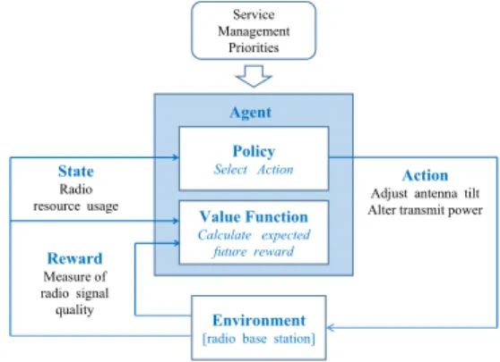
B. ACTIVE TECHNIQUES
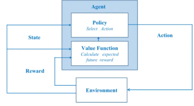
These are based on the principle ofreinforcement learning (RL), in which a part of the system known as the agent (see Fig. 4) takes actions on theenvironmentfrom which it receives reward signals, which are used to influence the next action.
The agent’s actions are determined by apolicy,which has to balance the benefits ofexploitation, in other words taking the action with the current highest expected future reward, againstexploration,which means taking another action with a lower currently expected future reward in order to seek even higher rewards in the future. To assist with this, another part of the system known as thevalue functionis used to estimate the total expected future reward of taking an action from a given system state. For a task such as compensation, where the goal is to achieve a stable result, the agent’s interaction
with the environment can be represented by a finite sequence called anepisode.
The two most popular RL techniques used in cell fault management are Q-learning [62] and Actor-Critic learning [33]. These have each been used to compensate for cell outages by adjusting the power levels and/or antenna tilt of neighbouring cells. They are both based on the Temporal Difference (TD) approach, in which the system evaluates the expected reward by looking ahead one step only. This gives the TD approach the advantage that it is not necessary to provide it with a model of the environment, as it can function by taking one action at a time and observing the outcome.
In Q-learning, the policy is fixed. A typical policy might specify that the system should normally take the action with the highest calculated future reward (exploitation), but in a small proportion of cases it should try another action (exploration). At each step of the process the value function for the action just taken, denoted by Q, is updated based on the feedback received from the environment. Hence Q is learned from experience as the system explores different actions, and at each step the most recent value of Q influences the system’s behaviour via the policy.
In the Actor-Critic approach, by contrast, the system mod-ifies the policy according to experience. The policy consists of a state-action table specifying the required probability of taking each action in a particular state. The critic forms an error signal comparing the outcome of a given action with the expected reward, which the actor uses to adjust the probability for this action in the policy table. So if the outcome of a particular action is positive, the probability of taking it again will be increased, but if the outcome is negative it will be decreased.
A key limitation of these RL techniques is that the size of the state-action table is proportional to the product of the number of system statessand the number of possible actions a which can lead to scalability issues. To address this, the deep RL technique introduces a deep neural network to carry out the mapping from states to actions [63]. The basic RL technique is then used to train the neural network to identify the action with the highest reward for each state, based on the experience of the RL subsystem. In order to average out the effect of specific conditions during a given episode, the state-action-reward data for each episode is stored in a replay memory to enable training samples for the neural network to be drawn randomly from multiple episodes.
C. ADVANTAGES, DISADVANTAGES AND CHALLENGES
In comparison with algorithmic solutions, ML approaches have the following general advantages and disadvantages.
Advantages:
1) built-in ability to process a much larger number of input features
2) can be retrained automatically eliminating the need for manual retuning
3) can be applied to a range of issues using standard libraries hence reduced need for specialist algorithm
expertise
4) reduced dependence on details of specific problem also reduces the need for domain knowledge
5) deep learning techniques can also dispense with much of the preprocessing code required by algorithmic methods and earlier ML approaches
Disadvantages:
1) significant volumes of training data required; collec-tion of sufficient fault data may be a substantial organ-isational challenge
In relation to logic based systems, similar advantages and disadvantages apply, with the following additions:
Advantages:
1) the ability to function without an explicit causal model removes the difficulty of maintaining consistency of a rule base as the problem domain becomes more complex
Disadvantages:
1) significantly more difficult to present reasoning in sup-port of recommendations
Hence the key challenges to overcome in support of the introduction of ML techniques are:
1) systematic collection of fault data
2) development of the ability of ML systems to explain and justify their recommendations
The first of these is primarily an organisational rather than a research issue and can be left to mobile network providers. The second has been recognised as a key blocker to progress and intensive research is now under way to address this, as we discuss below.
D. SUMMARY
In this section we have described the principal ML techniques which have been used in cell fault management, and for each group of techniques we have explained in broad terms which activity within fault management the techniques are most applicable to. We have covered at a high level the advantages, disadvantages and current challenges with ML techniques. In the next section we will drill down to look in more detail at the application of each technique to specific fault management activities and the specific strengths and limitations of each approach.
VII. APPLICATION OF MACHINE LEARNING TO FAULT MANAGEMENT IN CELLULAR NETWORKS
To date, much of the work on application of ML techniques to cellular network fault management has concentrated on the “sleeping cell" problem referred to in Section IV above, and related cell performance degradations [42] and [27]. Some recent work, however, has looked at more general faults in mobile networks [61].
Between them, the studies surveyed have covered detec-tion, diagnosis (action determination and root cause analy-sis) and compensation. For implementation in the network
Stage 1: Data Quality Enhancement Live Data Historic Data Noise Reduction Missing Data Compensation Screening Aggregation Sampling Anomaly Detector Reference Data Learn Model Parameters
Pre-Processing Fault Detection
Stage 2: Data Transformation Feature Engineering Data Fusion Dimensionality Reduction Feature Vectors If Fault Trigger Diagnosis
FIGURE 5. Preprocessing and Fault Detection
environment, all techniques require a further stage at the be-ginning which we can call pre-processing. In this section we review the ML techniques used by these studies, considering each stage in turn. For ease of reference, Table 13 at the end of this section lists all the studies presented here by stage(s) covered.
A. PRE-PROCESSING
The purpose of the pre-processing stage is to address the low level data quality issues identified in Section IV above and to transform the data into a form which can be utilised efficiently by the detection stage.
From the perspective of machine learning, we can identify two stages of pre-processing, as shown in Fig. 5. The purpose of stage 1 is to reduce data volume while improving the quality, and present the input data as a series of feature vectors as required by the ML subsystem. Stage 2, on the other hand, transforms the features for optimal processing by the ML subsystem.
1) Stage 1 - Data Quality Enhancement
Stage 1 techniques are used to address the low level data quality issues identified in Section IV above. Tailored digital filtering techniques may be used for noise reduction. Miss-ing data can be handled by missing data compensation, in which dummy or interpolated data is used to fill gaps which would otherwise disrupt processing. Specificscreeningcode may be implemented to remove irrelevant data.Aggregation techniques such as counting or accumulation of data values over a set period can be used to reduce the volume of data [29].Data samplingis used to transform an unlimited input time sequence into a finite set of vectors to enable the ML subsystem to treat the inputs as samples from a larger population. Typically a sliding window is used to capture successive sets of samples over a fixed time period [64].
2) Stage 2 - Data Transformation
Examples of Stage 2 techniques includefeature engineering, data fusionanddimensionality reduction.
The aim of feature engineering is to derive new features from the input data which can improve the performance of the
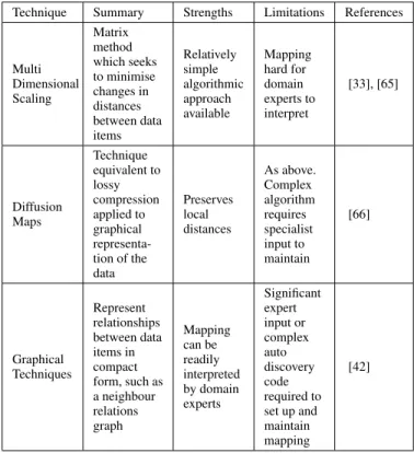
TABLE 6. Dimensionality Reduction Techniques In Fault Management Technique Summary Strengths Limitations References
Multi Dimensional Scaling Matrix method which seeks to minimise changes in distances between data items Relatively simple algorithmic approach available Mapping hard for domain experts to interpret [33], [65] Diffusion Maps Technique equivalent to lossy compression applied to graphical representa-tion of the data Preserves local distances As above. Complex algorithm requires specialist input to maintain [66] Graphical Techniques Represent relationships between data items in compact form, such as a neighbour relations graph Mapping can be readily interpreted by domain experts Significant expert input or complex auto discovery code required to set up and maintain mapping [42]
ML subsystem or allow a technique to be used in situations where it would not otherwise be applicable. One example of feature engineering is the use of a Fast Fourier Transform (FFT) to detect periodic variations in a time sequence [29]. Another example is where polynomial terms are formed from the basic features, so that a non-linear boundary in the input feature space can be transformed into a linear boundary in the polynomial space.
Data fusion, on the other hand, addresses the situation where any individual data item is weakly correlated with the occurrence of a fault or one of its causes; by combining two or more data items it may be possible to produce a feature with higher correlation than any of its components.
Dimensionality reduction is needed where the number of input dimensions is sufficient to cause degradation of the ML system performance. It is particularly useful for removing redundant information in the case where different features are partially correlated with each other. The goal is to reduce the number of features while retaining as much of the key information from the input as possible. Three key techniques which have been applied to fault management are listed in Table 6.
At the current state of the art, the preprocessing phase requires a significant level of hand coding to tune the front end to match the input data to the ML technique being used. This typically requires scarce specialist effort and can limit system flexibility in response to change.
B. DETECTION
The purpose of the detection stage is to determine whether a fault is present or not, without committing significant resources to diagnosis and compensation until a reliable decision has been made.
There are now many instances where ML approaches, both parametric and non parametric, have been proposed for use in detecting faults in cellular networks. These assume as a minimum that a set of data is available representing normal operation, against which anomalies representing faults can be detected. All these techniques operate at the correlation level, in other words they are not dependent on the availability of a causal model of the network.
A sleeping cell situation arises where a radio failure is not being reported to the network management system. Hence sleeping cell failures have to be detected indirectly, using related evidence such as radio signal strength, channel qual-ity indicators and higher level indicators such as incoming handovers and dropped call rates. Similar data may be used to detect other anomalies, such as misconfigured parameters which impact the extent and quality of the radio coverage.
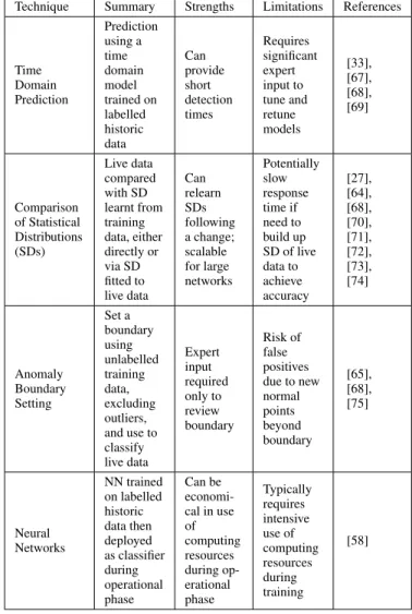
Parametric techniques described in the literature are listed in Table 7. In Time Domain Prediction, a KPI is compared with a predicted value at each time step. Three examples of this approach are network calculus, Auto Regressive In-tegrated Moving Average (ARIMA) modelling, and Grey modelling. In each case previous data from the sequence, representing normal operation, is used to learn the settings of the model parameters which minimise the prediction error.
Comparison of Statistical Distributions takes place be-tween the live KPI data and a reference data set representing normal operation. To achieve this, it is necessary to fit a statis-tical distribution to the normal reference data set then either: (a) compare live KPI data directly with the stored distribution to generate a normalised “KPI level" representing the degree of abnormality of the relevant KPI or (b) fit a second distri-bution to the live data then either compare parameters with the stored distribution or compare the distributions directly.
Parametric Binary Classification is based on a labelled training dataset including both normal and fault data. Two approaches to achieve this are described in [42]. The first uses the Classification and Regression Tree (CART) technique to recursively partition the data into normal and anomalous regions to be used for classification of live data. The second, by contrast, uses a Linear Discriminant Function (LDF) to learn the parameters of a hyperplane to be used to separate normal and anomalous data.
In Anomaly Boundary Setting, a boundary is set between normal and anomalous data on an unlabelled normal training data set by excluding a specified number of outliers. The boundary is then used to classify live data as normal or anomalous. In [65] and [68], this is done by using a one class Support Vector Machine (SVM) which works generally as described in Section VI above. In the specific case of the one class SVM, the budget is used to allow a small number of outliers in the normal data to be misclassified as faults, in
TABLE 7. Parametric Approaches to Fault Detection
Technique Summary Strengths Limitations References
Time Domain Prediction Prediction using a time domain model trained on labelled historic data Can provide short detection times Requires significant expert input to tune and retune models [33], [67], [68], [69] Comparison of Statistical Distributions (SDs) Live data compared with SD learnt from training data, either directly or via SD fitted to live data Can relearn SDs following a change; scalable for large networks Potentially slow response time if need to build up SD of live data to achieve accuracy [27], [64], [68], [70], [71], [72], [73], [74] Anomaly Boundary Setting Set a boundary using unlabelled training data, excluding outliers, and use to classify live data Expert input required only to review boundary Risk of false positives due to new normal points beyond boundary [65], [68], [75] Neural Networks NN trained on labelled historic data then deployed as classifier during operational phase Can be economi-cal in use of computing resources during op-erational phase Typically requires intensive use of computing resources during training [58]
order to achieve optimum anomaly detection performance on live data. In [75], anomaly boundary setting is done by fitting a Gaussian distribution to normal data.
With NNs used as classifiers, the network weights are optimised by against labelled normal and fault data. Once trained, the NN can then be used to classify incoming live data.
Feng et al. used a feedforward NN as a classifier in a cell detection scenario; they encountered difficulties due to the system becoming trapped in non-optimal local minima during training, degrading system accuracy. This was re-solved by using a “differential evolution" algorithm as the NN optimiser [58].
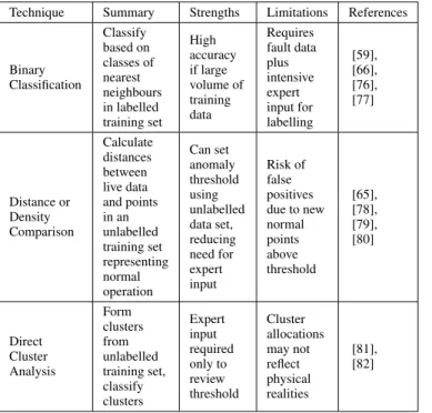
Non-parametric techniques described in the literature are listed in Table 8. In non-parametric Binary Classification, anomaly detection is again treated as a binary classification problem using labelled training data representing normal and faulty operation. In this case, however, each live data point is classified as normal or anomalous by identifying itsknearest neighbours in the training set and then classifying it based on the majority of the neighbour classifications.
TABLE 8. Non Parametric Approaches to Fault Detection
Technique Summary Strengths Limitations References
Binary Classification Classify based on classes of nearest neighbours in labelled training set High accuracy if large volume of training data Requires fault data plus intensive expert input for labelling [59], [66], [76], [77] Distance or Density Comparison Calculate distances between live data and points in an unlabelled training set representing normal operation Can set anomaly threshold using unlabelled data set, reducing need for expert input Risk of false positives due to new normal points above threshold [65], [78], [79], [80] Direct Cluster Analysis Form clusters from unlabelled training set, classify clusters Expert input required only to review threshold Cluster allocations may not reflect physical realities [81], [82]
Distance or Density Comparison uses a training data set representing normal operation only. In this method, anoma-lies are detected either: (a) by computing some function of the distances from theknearest neighbours in the training set and comparing this with a threshold or (b) by calculating the local data density (the number of points in unit volume of the feature space) for each live data point and comparing it with the global average density, or the average density of its knearest neighbours.
Oniretiet al.(see Table 12 below) report that in a macro-cell scenario, the globalkthnearest neighbour approach was more accurate than a local density based method [33].
Direct Cluster Analysis employs an unlabelled training data set representing both normal and faulty operation. This technique forms clusters from the training data and classifies the clusters (as opposed to the raw data) as normal or anoma-lous using other KPIs which differ in value between normal and anomalous operational states. Anomaly detection is then carried out by comparing the distances of each live data point to the normal and anomalous clusters.
The two types of training method have different strengths and weaknesses from a RAN deployment perspective. Para-metric techniques require access to a central database during the initial training phase. Once the parameters have been learned, however, the system can in principle be deployed in the RAN without the need for further access to central data. Non parametric techniques, on the other hand, do not require an initial training phase but during live operation do require access to a central historic fault database.
Fault Category plus Recommended Action Live Data (Fault Symptoms) Cluster Analysis Reference Data (Normal Operation and Fault Conditions) Fault Clusters Classifier Expert Input
FIGURE 6. Action Determination using Cluster Analysis
TABLE 9. Approaches to Fault Diagnosis 1: Action Determination
Technique Summary Strengths Limitations References
Network Based with Causal Model Build a model of network symptom cause relationships and use to identify the most likely cause of a given fault Relatively simple to explain the output For complex networks may become infeasible to build and maintain causal model [83], [70], [84], [85], [86] Network Based without Causal Model Work directly with network symptom cause data exploiting correlations between symptoms and causes Has the potential to scale to very large and complex networks Difficult to provide rationale for output [27], [66], [82], [87], [60] Operator Action Analysis Analyse operator action record to directly identify successful actions in response to given symptoms No need to gather network data; can quickly devise strategies to correct most common faults May be difficult to identify whether action successful or not; may be slow to adapt as network changes [88]
C. DIAGNOSIS 1: ACTION DETERMINATION
Upon detecting a symptom, the task of action determination is to identify appropriate compensation actions in order to restore normal service as far as possible. In earlier studies, there was an attempt to construct a detailed causal model to support this. In more recent work, however, there has been a trend away from this towards a “black box" approach working at the correlation level. Approaches described in the literature are listed in Table 9.
A popular approach to diagnosis from the earliest studies onwards is to use the Bayesian Networks/Naive Bayesian Classifier method described in Section VI above. In this
approach, typically the expert is needed at the start to define the logical relationships from which the network is built, but the probabilities required can then be extracted from historic data, if this is available [83], [70], [84], [85] and [86].
The use of the Naive Bayesian Classifier assumes that only one cause is present at a time and that the symptoms are independent given the cause. The studies acknowledge that this is likely to be unrealistic for some faults in an actual network but nonetheless report acceptable diagnostic performance for the scenarios studied.
Symptoms may be presented to the classifier in continuous form or alternatively they may be discretised first using one or more thresholds to generate binary values. The threshold levels can be set automatically using an ML technique called Entropy Minimisation Discretisation (EMD) [83]. Barco et al. conclude that the continuous approach is preferable if large fault data sets are available, whereas if only small data sets are available the discrete approach should be used [85]. Another method is to retain the conditional probability calcu-lations from the BN approach while relaxing the requirement to build an explicit causal model. In contrast with the BN approach to symptom data, Szilagyiet al.begin by deriving a KPI level, which is a standardised measure of the deviation of the current KPI value from that for normal operation [27]. The system then calculates the likelihood that the cause is present given each symptom (based on historic relative frequencies), and multiplies this by the KPI level to give a score for each candidate cause.
A more radical option is to directly classify the symptoms from historic data, in which each symptom is labelled with a cause, but without constructing a causal model. In [66], the knearest neighbours approach is used to classify incoming symptom sets based on the classes of theirknearest neigh-bours in the training set.
More recently a hybrid approach has been put forward (see Fig. 6), which is to carry out a cluster analysis on the symptoms first, then use a network approach to relate the clusters of symptoms to potential causes. Ciocarlie et al. used a Hierarchical Dirichelet Process for the cluster analysis and an Markov Logic Network for classification [82]. They set up the network manually after which the system learnt the weightings from a training data set based on maximum likelihood estimation. Gomez-Andrades et al. used a self organising map to carry out the cluster analysis [87] and [60]. This maps a dataset of continuous data to a set of discrete points representing the clusters. After a degree of automatic quality checking, the clusters are verified by an expert before being used for classification of live data. Although this does require a degree of expert input, the effort required is very much less than if the clustering had not been carried out first. A recent paper related to cellular networks, however, has taken a radically different approach to action determination [88]. The aim here is to automatically learn service manage-ment policies and rules for triggering compensation actions, from historic logs of faults and related operator actions. Symptoms are detected from anomalies in a rolling time
Service Management
Priorities
Action Adjust antenna tilt Alter transmit power
Environment [radio base station] State Radio resource usage Reward Measure of radio signal quality Agent Value Function Calculate expected future reward Policy Select Action
FIGURE 7. Compensation using Reinforcement Learning
TABLE 10. Approaches to Compensation
Technique Summary Strengths Limitations References
Q Learning Fixed policy: normally take action with highest expected reward but sometimes try different action; expected reward per action updated at each step. Able to learn from experience without the need to build an explicit model of the network Relatively slow to converge. Either need to learn on part of the actual network where learning can be tolerated or against a simulator [89], [62], [90] Actor-Critic Policy updated at each step; probability of taking a given action adjusted to reflect the outcome when it was last taken. As above Faster to converge; same learning issue as above [33], [91]
sequence of key KPIs and associated with successful actions occurring within a time window of the anomaly; a logistic regression classifier is then trained from this data and used to classify new symptoms according to the action required. No attempt is made to determine the cause; the system operates at the correlation level and only considers what action pre-viously resolved the problem. It is critical to this approach to consider only successful operator interventions based on the subsequent outcome; in some cases expert review of the historic logs is likely to be required to determine which these are.
D. COMPENSATION
The aim of compensation is to restore the best possible level of service given the remaining serviceable network resources, according to priorities set by a policy specified by the network operator.