Physical programming for preference driven evolutionary multi-objective optimization

(1)

Document downloaded from:

This paper must be cited as:

The final publication is available at

Copyright

Additional Information

http://hdl.handle.net/10251/57265

Elsevier

Reynoso Meza, G.; Sanchís Saez, J.; Blasco Ferragud, FX.; Garcia Nieto, S. (2014). Physical programming for preference driven evolutionary multi-objective optimization. Applied Soft Computing. 24:341-362. doi:10.1016/j.asoc.2014.07.009.

(2)

Physical Programming for Preference Driven Evolutionary

Multi-Objective Optimisation

Gilberto Reynoso-Meza a,∗_{, Javier Sanchis}a_{, Xavier Blasco} a_{, Sergio Garc´ıa-Nieto}a a

Instituto Universitario de Automática e Informática Industrial, Universitat Politècnica de València, Camino de Vera s/n , Valencia 46022, Spain

Abstract

Preference articulation in multi-objective optimisation could be used to improve the pertinency of solutions in an approximated Pareto front. That is, computing the most interesting solutions from the designer’s point of view in order to facilitate the Pareto front analysis and the selection of a design alternative. This articulation can be achieved in an a

priori, progressive, or a posteriori manner. If it is used within an a priori frame, it could

focus the optimisation process towards the most promising areas of the Pareto front, saving computational resources and assuring a useful Pareto front approximation for the designer. In this work, a physical programming approach embedded in an evolutionary multi-objective optimisation is presented as a tool for preference inclusion. The results presented and the algorithm developed validate the proposal as a potential tool for engineering design by means of evolutionary multi-objective optimisation.

Keywords: Multi-objective optimisation design procedure, evolutionary multi-objective

optimisation, physical programming, many-objective optimisation, preference articulation, decision making.

1. Introduction

Multi-objective optimisation design (MOOD) procedures are generate first choose later

(GFCL) holistic strategies for multi-objective problems [1]. A multi-objective problem (MOP) arises when multiple objectives and requirements must be fulfilled by the designer. Such objectives are usually in conflict with each other; therefore a trade-off solution must be calculated and selected for implementation. The GFCL strategy generates a set of po-tentially preferable design alternatives and the decision maker (DM or simply the designer) selects the most preferable solution according to his or her preferences. These solutions are generally Pareto optimal solutions [2].

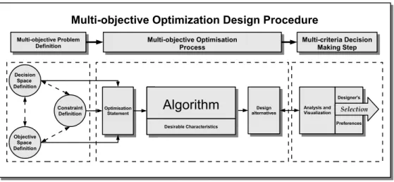
The MOOD procedure (see Figure 1) identifies three main (possibly fundamental) steps [3, 4]: the MOP definition (measure); the multi-objective optimisation process (search); and

∗_{Corresponding author. Tel.:+34963877007;fax:+34963879579}

Email address: [email protected](Gilberto Reynoso-Meza )

(3)

the multi-criteria decision making (MCDM) step (decision making). Major efforts are made to improve the algorithms and tools to facilitate the two latter processes.

In the case of multi-objective optimisation, several algorithms have been designed (NBI [5], NNC1 _{[6, 7], NSGA-II}2 _{[8], MOGA}3 _{[9], MOEA/D}4 _{[10] for example) and used in a wide}

variety of applications [11, 12, 13, 14, 15, 16, 17, 18, 19, 20, 21, 22, 23, 24]. Such algorithms mainly seek a set of Pareto optimal solutions that describe a Pareto front approximation. According to the designer’s wishes, those algorithms would incorporate some desirable char-acteristics [23] such as convergence (capacity to reach the Pareto front), diversity (capacity to generate different solutions), and pertinency (capacity to generate useful solutions for the DM). For the decision making step, several tools and visualisations approaches [25] have been proposed over the years (scatter plot diagrams, parallel coordinates [26], level diagrams [27, 28] or self-organizing maps [29] for example).

In [30, 31] the importance of considering both processes (optimisation and selection) in a holistic way, in order to guarantee a full embedment of the DM in the decision making step, was noted. This is because the decision making process is usually more time consuming than the optimisation step [32]. This embedment could be achieved by providing a useful set of solutions to the designer; thereby analysing the trade-off between conflicting objectives in order to refine his or her final selection [30].

Figure 1: A multi-objective optimisation design (MOOD) procedure.

Given that the MOOD procedure should be a holistic technique, preference handling mechanisms could play a major role in bridging the gap between optimisation and the se-lection process. These mechanisms will enable the algorithm to approximate a Pareto front with pertinent solutions in the search process; and therefore facilitating the DM’s task of

1

Matlab code available athttp://www.mathworks.com/matlabcentral/fileexchange/38976 2

Source code available at: http://www.iitk.ac.in/kangal/codes.shtml; also, a variant of this algo-rithm is available in the global optimisation toolbox of Matlab.

3

Toolbox for Matlab available athttp://www.sheffield.ac.uk/acse/research/ecrg/gat 4

(4)

analysing and selecting a design alternative [33]. Furthermore, preference handling might be used in constrained optimisation instances and many-objective optimisation statements [34]. Challenges for preference articulation include building a practical framework to link the designer’s desired trade-off with the cost function to optimise.

A first step for the aforementioned challenge, is stating meaningful design objectives. Sometimes with classical optimisation approaches a cost function (or objective) is built in order to satisfy a set of requirements such as convexity and/or continuity; that is, it is built from the point of view of the optimiser despite a possible loss of interpretability. The usage of more interpretable objectives facilitates the inclusion of preferences in the optimisa-tion process, producing meaningful and pertinent soluoptimisa-tions for the designer in the selecoptimisa-tion step. Evolutionary multi-objective optimisation (EMO) provides a helpful framework for this purpose, since multi-objective evolutionary algorithms (MOEAs) have been shown to be a flexible tool to handle constrained complex functions [32] in a wide variety of engi-neering domain applications [11]. Furthermore, a convenient feature of using MOEAs is the possibility of selecting more interpretable objectives for the designer. That is, the objective selection could be closer to the point of view of the designer, rather than the optimiser. Nevertheless, this is just a necessary step to moving forward to preference articulation, since this could assure meaningful, but not pertinent, design alternatives.

The physical programming (PP) method [35] is very suitable for multi-objective en-gineering design since it formulates design objectives in an understandable and intuitive language for designers. Since it defines desirable, tolerable, and undesirable ranges for in-dividual objectives, it becomes a potential technique to improve the pertinency of solutions in multi-objective optimisation. PP has been merged previously with classical optimisation techniques [1, 36]; nevertheless, it remains an interesting topic to merge with MOEAs.

In this work, PP is merged with MOEAs as an auxiliary mechanism to improve the pertinency of the calculated solutions. Such an approach will enable the DM to have more useful solutions, since it provides a flexible and intuitive coding framework where the MOP is built from the DM’s point of view. Although an algorithm to test its viability is developed, it could be incorporated in other MOEAs. The remainder of this work is as follows: in Section 2 several preliminaries in multi-objective optimisation, physical programming, and the MOEA are presented. In Section 3 the preference handling mechanism is explained, and then evaluated in Section 4. Finally, some concluding remarks are given.

2. Background

To state the proposal, some notions on multi-objective optimisation, preference handling, physical programming, and the algorithm to be used are required. Those are provided below.

2.1. Multi-objective optimisation review

As referred in [2], a MOP 5_{, can be stated as follows:}

5

A maximization problem can be converted to a minimization problem. For each of the objectives that have to be maximized, the transformation: maxJi(θ) =−min(−Ji(θ)) could be applied.

(5)

min θ J(θ) = [J1(θ), . . . , Jm(θ)] (1) subject to: K(θ) ≤ 0 (2) L(θ) = 0 (3) θi ≤θi ≤ θi, i= [1, . . . , n] (4)

where θ = [θ1, θ2, . . . , θn] is defined as the decision vector with dim(θ) =n; J(θ) as the

objective vector and K(θ), L(θ) as the inequality and equality constraint vectors respec-tively; θi, θi are the lower and upper bounds in the decision space.

It has been pointed out that there is not a single solution in MOPs, because there is not generally a better solution in all the objectives. Therefore, a set of solutions, the Pareto set, is defined. Each solution in the Pareto set defines an objective vector in the Pareto front. All the solutions in the Pareto front are a set of Pareto optimal and non-dominated solutions:

Definition 1. (Pareto optimality [2]): An objective vector J(θ1) is Pareto optimal if there

does not exist another objective vectorJ(θ2₎_{such that} _J

i(θ2)≤Ji(θ1)for alli∈[1,2, . . . , m] and Jj(θ2)< Jj(θ1) for at least one j, j ∈[1,2, . . . , m].

Definition 2. (Dominance [11]): An objective vector J(θ1₎_{is dominated by another}

objec-tive vector J(θ2) iff Ji(θ2)≤Ji(θ1) for all i∈[1,2, . . . , m] and Jj(θ2)< Jj(θ1) for at least

one j, j ∈[1,2, . . . , m]. This is denoted as J(θ2)J(θ1).

Definition 3. (Strict dominance): An objective vector J(θ1) is strictly dominated by

an-other objective vector J(θ2) if Ji(θ2) < Ji(θ1) for all i ∈ [1,2, . . . , m]. This is denoted as

J(θ2)≺J(θ1).

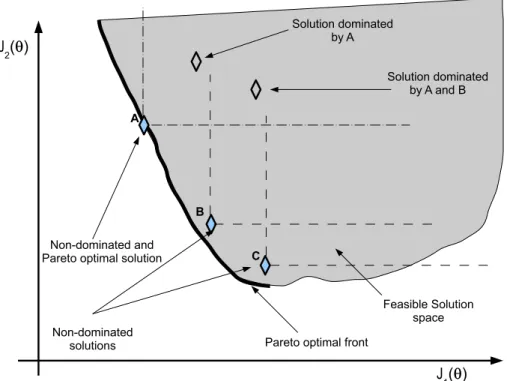
For example, in Figure 2, five different solutions (♦) are calculated in order to approx-imate a Pareto front (bold line). Solutions A, B and C are non-dominated solutions, since there is not a better solution vector (in the calculated set) for all the objectives. Solutions B and C are not Pareto optimal, since some solutions (not found in this case) (strictly) dominate them. Furthermore, solution A is also Pareto optimal, since it lies on the feasible Pareto front. The set of non-dominated solutions built the Pareto front approximation J∗

P.

It is important to notice that the Pareto front is usually unknown, and the DM can only rely on Pareto front approximations.

2.2. Background on preference handling in multi-objective optimisation

As commented before, one potentially desirable characteristic of a MOEA is the mecha-nism for preference handling in order to calculate pertinent solutions. That is, the capacity to obtain a set of interesting solutions from the DM’s point of view (Figure 3). Incorporating

(6)

Figure 2: Pareto optimality and dominance concepts.

(7)

the DM’s preferences into MOEAs has been suggested to improve the pertinency of solutions (see for example [33, 37]).

The designer’s preferences could be defined in the MOOD procedure in an a priori,

progressive, or a posteriori fashion [38].

• A priori: the designer has partial knowledge about his or her preferences in the design

objective space. In such cases, the DM could be interested in using an algorithm that enables incorporating such preferences in the optimisation procedure.

• Progressive: the optimisation algorithm embeds the designer into the optimisation

process to adjust or change his or her preferences on the fly. This could be a desirable characteristic for an algorithm when the designer has some knowledge of the objective trade-off in complex problems.

• A posteriori: the designer analyses the Pareto front calculated by the algorithm, and

according to the set of solutions, he or she defines the preferences in order to select a preferable solution.

It is also possible to classify preference handling techniques into five classes with respect to the question: what it is important for the designer?:

Dominance is essential: it is important for the designer to calculate a set of solutions that dominate one or morereference objective vectors.

Objective against objective: it is important for the designer to identify which objectives have priority over others through the EMO process.

Objective value against objective value: it is important for the designer to identify when the value of a given objective has priority over the value of others.

Subset against subset: identifying a combination of objectives and values that are pre-ferred over others.

Some popular techniques include ranking procedures, goal attainment, and fuzzy relations [33]. Possibly one of the first algorithms to include preference information is the MOGA [39, 40] algorithm which uses a goal vector scheme. In [41], the NSGA-II algorithm is improved using preferences in a fuzzy scheme. Other examples are presented in [42] where a preference information approach was merged with the IBEA proposal; or in [40] where a preference articulation technique is used in the MOGA framework. Examples where the ranking scheme has been used include [43, 44, 45, 46]. In any case, some desirable characteristics of the preference handling mechanism have been stated in [47]:

• Handling multiple preference conditions simultaneously.

(8)

• The handling mechanism should be indifferent to the shape of the Pareto front. • It should be capable of handling many-objective optimisation instances.

Here, the following feature is also considered:

• It should enable the DM to decide how many solutions are required in the Pareto front approximation, which will be analysed in the MCDM step.

In this paper, an implementation using physical programming as ana priori technique for preference handling in EMO is presented. Such implementation will incorporate modifica-tions in order to cover the features discussed above. A brief review of physical programming is presented below.

2.3. Physical programming review

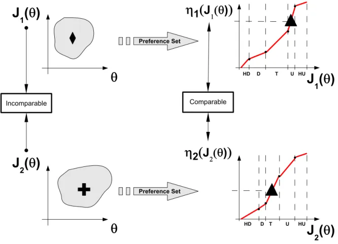
The physical programming (PP) method is a suitable technique for multi-objective en-gineering design since it formulates design objectives in an understandable and intuitive language for designers. PP is an aggregate objective function (AOF) technique [31] for multi-objective problems that includes the available information in the optimisation phase. This enables the designer to express preferences relative to each objective function with more detail. Firstly, PP translates the designer’s knowledge into classes6 _{with previously defined}

ranges.7 _{This preference set reveals the DM’s wishes using physical units for each of the}

objectives in the MOP. From this point of view, the problem is moved to a different range where all the variables are independent of the original MOP (see Figure 4).

For each objective and set of preferencesP, a class function ηq(J(θ))|_P,q= [1, . . . , m] is

built to translate each objective Jq(θ) to a new range where all the objectives are equivalent

to each other. A PP index Jpp(J(θ)) = m P q=1

ηq(J(θ)) is then calculated.

For example, in Figure 4, two objectivesJ1(θ) andJ2(θ) are optimised (in both cases: the

smaller, the better). At this point, there is not enough information to compare two objective

values J1(θ) = a against J2(θ) = b; nevertheless, using a preference set, it is possible to

map each objective to a certain range of preferences and so enable the comparison. In this exampleJ1(θ) =ais in the undesirable region (U) andJ2(θ) =bis in the tolerable zone (T).

Therefore, it is possible to compare both objective valuesaandb: bisless desirablethana; by assigning numerical values in this new range, it is possible for an algorithm interpreting these semantic values to perform a preference based optimisation. This information is exploited by the optimiser, for example, by means of the OVO (one-vs-others) rule of the original PP technique: some degradation will be accepted in the objective J2(θ) if that implies a better

6

The original method states 4 classes: 1S (smaller is better); 2S (larger is better); 3S (a value is better); and 4S (a range is better)

7

According to the original method: highly desirable (HD), desirable (D), tolerable (T), undesirable (U) and highly undesirable (HU)

(9)

Figure 4: Physical programming (PP) notion. Five preference ranges have been defined: highly desirable (HD), desirable (D), tolerable (T) undesirable (U) and highly undesirable (HU).

(10)

performance of J1(θ) with the aim of placing both values in the tolerable region. This is

achieved by optimizing the Jpp(J(θ)) =η1(J1(θ)) +η2(J2(θ)) index.

In this work, the implementation stated in [48], namely Global Physical Programming (GPP), is a better fit for evolutionary optimisation techniques and will be used. This is due to the fact that the original method employs several resources to build the proper class functions

ηq(J(θ))|_P, to fulfill a list of convexity and continuity requirements. The interested reader

might refer to [48, 49] for a detailed explanation. For the sake of simplicity such details are not reproduced here, since they will be used as a basis for the development to be presented in Section 3.

The Jpp(J(θ)) index is suitable to evaluate the performance of a design alternative, but

not that of the design concept. That is, if it is used as it is, it will evolve the entire population to a single Pareto optimal solution. Therefore, it must be merged with other mechanisms to maintain diversity in the Pareto front. Pruning mechanisms seem to be a promising solution for this purpose. Therefore, GPP will be used with the spMODE algorithm (see Algorithm 4 in the next section and references [50, 51]), which is a MOEA based on the differential evolution algorithm [52, 53, 54] and spherical coordinates to prune J∗

P. Even if

similar algorithms use similar approaches [55, 56, 57], the usage of a norm to perform the pruning makes it suitable to incorporate preferences, as detailed below.

2.4. Spherical pruning review

A general pseudocode for MOEAs with pruning mechanism and external archive A is shown in Algorithm 1. The usage of an external archive A to store the best set of quality solutions found so far in an evolutionary process is common in EMO.

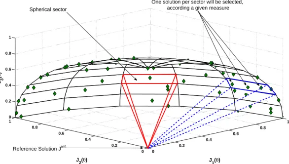
The basic idea of the spherical pruning is to analyze the proposed solutions in the current Pareto front approximation J∗

P by using normalized spherical coordinates from a reference

solution (see Figure 5). With such an approach, it is possible to attain a good distribution along the Pareto front [50, 51]. The algorithm selects one solution for each spherical sector (see Figure 5), according to a given norm or measure. This process is explained in Algorithm 2, where the following definitions are required:

Definition 4. (normalized spherical coordinates) given a solution θ1

and J(θ1

), let

S(J(θ1)) = [kJ(θ1)k2,β(J(θ 1

))] (5)

be the normalized spherical coordinates from a reference solution Jref where β(J(θ1

)) = [β1(J(θ1)), . . . , βm−1(J(θ1))] is the arc vector and kJ(θ1)k2 the Euclidean distance to the

reference solution.

It is important to guarantee thatJref dominates all the solutions. An intuitive approach is to select:

Jref =Jideal =minJ1(θ

i

), . . . ,minJm(θ i

(11)

0 0.2 0.4 0.6 0.8 1 0 0.2 0.4 0.6 0.8 1 0 0.2 0.4 0.6 0.8 1 J 1(θ) J₂(θ) J 3 ( θ )

Reference Solution Jref Spherical sector

One solution per sector will be selected, according a given measure

Figure 5: Spherical relations onJ∗

P ⊂R 3

. For each spherical sector, just one solution, the solution with the lowest norm will be selected.

Definition 5. (sight range) The sight range from the reference solution Jref to the Pareto

front approximation J∗ P is bounded by β U and βL : βU =maxβ1(J(θ i )), . . . ,minβm−1(J(θ i )) ∀ J(θi)∈Aˆ|G (7) βL=minβ1(J(θ i )), . . . ,minβm−1(J(θ i )) ∀ J(θi)∈Aˆ|G (8)

If Jref =Jideal, it is straightforward to prove that βU =π₂, . . . ,π₂ and βL = [0, . . . ,0].

Definition 6. (spherical grid) Given a set of solutions in the objective space, the spherical

grid on the m-dimensional space in arc increments βǫ = [β₁ǫ, . . . , β_mǫ₋₁] is defined as:

ΛJ∗ P = βU 1 −β1L βǫ 1 , . . . , β U m−1−βmL−1 βǫ m−1 (9)

Definition 7. (spherical sector) The normalized spherical sector of a solution θ1

is defined as: Λǫ(θ 1 )= "& β1(J(θ 1 )) ΛJP∗ 1 ' , . . . , & βm−1(J(θ 1 )) ΛJP∗ m−1 '# (10)

Definition 8. (spherical pruning) given two solutionsθ1

and θ2

from a set, θ1

has

prefer-ence in the spherical sector over θ2

if: Λǫ(θ 1 )=Λǫ(θ 2 )∧kJ(θ1)kp <kJ(θ 2 )kp (11)

(12)

1 Generate initial population P|₀ with N_p individuals; 2 Evaluate P|₀;

3 Apply dominance criterion on P|₀ to obtain archive A|₀; 4 while stopping criterion unsatisfied do

5 Update generation counter G=G+1;

8 Evaluate offspring O|_G;

9 Update population P|_G with offspring O|_G;

12 Update environment variables (if using a self-adaptive mechanism);

13 end

14 Algorithm terminates. J_P is approximated by J∗

P =A|G;

Algorithm 1:MOEA with pruning mechanism

where kJ(θ)kp = _m P q=1 |Jq(θ)|p 1/p is a suitable p-norm.

In this implementation, spherical pruning is merged with the DE algorithm [52, 54, 58]. Although any other evolutionary or nature-inspired mechanism may be used, the DE algo-rithm was selected because of its simplicity. The DE algoalgo-rithm uses two operators: mutation and crossover (Equations (12) and (13) respectively) to generate its offspring (Algorithm 3).

Mutation: For each target (parent) vector θi|G, a mutant vector vi|G is generated at

generation Gaccording to Equation (12):

vi|G =θr1|G+F(θr2|G−θr3|G) (12)

Where r1 6=r2 6=r3 6=i and F is usually known as the scaling factor.

Crossover: For each target vector θi|G and its mutant vector vi|G, a trial (child) vector

where j ∈1,2,3. . . n and Cr is named the crossover probability rate. The standard selection mechanisms are as follows:

• For single objective optimisation, a child is selected over its parent (for the next gen-eration) if it has a better cost value.

(13)

1 Read archive ˆA|_G;

2 Read and update extreme values for J_ref|_G;

3 for each member in Aˆ|_G do

4 calculate its normalized spherical coordinates (Definition 3);

5 end

6 Build the spherical grid (Definition 4 and 5);

8 calculate its spherical sector (Definition 6);

9 end

10 for i=1:SolutionsInArchive do

11 Compare with the remainder solutions in ˆA|_G;

12 if no other solution has the same spherical sector then

13 it goes to archive A|_G₊₁;

14 end

15 if other solutions are in the same spherical sector then

16 it goes to archive A|_G₊₁ if it has the lowest norm (Definition 7);

17 end

18 end

19 Return Archive A|_G₊₁;

Algorithm 2: Spherical pruning mechanism

1 for i=1:SolutionsInParentPopulation do

2 Generate a Mutant Vector vi (Equation (12)) ; 3 Generate a Child Vector ui (Equation (13)) ;

4 end

5 Offspring O =U;

(14)

• In EMO, a simple selection based on dominance is used; a child is selected over his parent if the child dominates his parent (Definition 3).

3 Apply dominance criterion on P|₀ to obtain A|₀; 4 while stopping criterion unsatisfied do

5 Read generation count G;

6 Obtain subpopulation S|_G with solutions in P|_G and A|_G;

7 Generate offspring O|_G with S|_G using DE operators (Algorithm 3).; 8 Evaluate offspring O|_G;

9 Update population P|_G with offspring O|_G according to greedy selection

mechanism.;

10 Apply dominance criterion on O|_GSA|_G to obtain ˆA|_G;

11 Apply pruning mechanism based on spherical pruning (Algorithm 2) to prune ˆA|_G

to obtain A|G+1;

12 G=G+ 1;

13 end

P =A|G;

Algorithm 4: spMODE.

This solution, merging the DE algorithm and the spherical pruning mechanism (Algo-rithm 2) was termed the spMODE algo(Algo-rithm (see Algo(Algo-rithm 4) and it is freely available at Matlab c Central8_{. At this point, we will present the preference handling proposal of this}

paper.

3. Pertinency Improvement by means of GPP

Global physical programming is a tool that can be used in different ways by MOEAs. In this case, it will be merged together with a pruning technique, in order to decide which solutions will be archived in an external file. GPP can be used as a selection mechanism in the evolved population and/or in the store and replace the mechanism in the external archive A.

3.1. Global physical programming statements

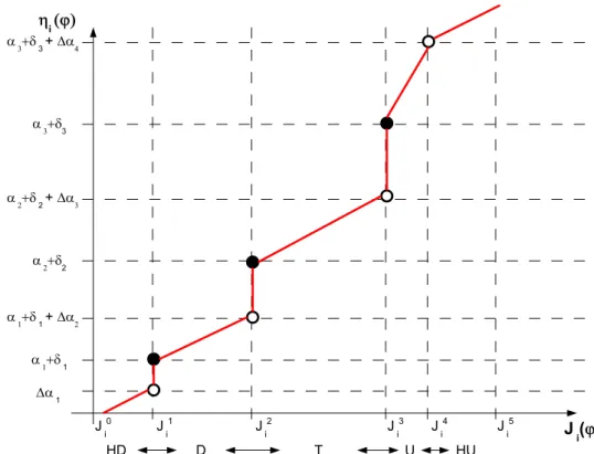
Given a vector ϕ ∈ Rm, linear functions will be used for class functions ηq(ϕ)|P as

detailed in [48]9_{, due to their simplicity and interpretability. Firstly, an offset between two}

8

http://www.mathworks.com/matlabcentral/fileexchange/39215 9

(15)

adjacent ranges is incorporated (see Figure 6) to meet the OVO rule criterion [59, 60]. Given a set of preferences P with M ranges form objectives:

P=    J1 1 · · · J1M .. . . .. ... J1 m · · · JmM    (14)

ηq(ϕ)|_P, q = [1, . . . , m] are defined as:

ηq(ϕ)|_P = αk−1+δk−1+ ∆αk ϕq−Jqk−1 Jk q −Jqk−1 (15) J_qk−1 ≤ϕq < Jqk (16) where α0 = 0 (17) α1 ∈ R+ (18) αk > αk−1 (1< k≤M) (19) ∆αk = αk−αk−1 (1≤k ≤M) (20) δ0 = 0 (21) δ1 ∈ R+ (22) δk > m·(αk+δk−1) (1< k≤M) (23)

The last inequality guarantees the OVO rule, since an objective value in a given range is always greater than the sum of the others in a more preferable range. Therefore, theJgpp(ϕ)

index is defined as:

Jgpp(ϕ) = m X q=1

ηq(ϕ)|_P (24)

The Jgpp(ϕ) has an intrinsic structure to deal with constraints. If the fulfillment of

constraints is required, they will be included in the preference set as objectives. That is, preference ranges will be stated for each constraint and they will be used to compute the

Jgpp(ϕ) index. The ηq(ϕ)|P is shown in Figure 6 for the specific case (to be used hereafter)

of the following 5 preference ranges:

HD: Highly desirable if J0 q ≤Jq(ϕ)< Jq1. D: Desirable if J1 q ≤Jq(ϕ)< Jq2. T: Tolerable if J2 q ≤Jq(ϕ)< Jq3.

(16)

U: Undesirable ifJq3 ≤Jq(ϕ)< Jq4.

HU: Highly undesirable J4

q ≤Jq(ϕ)< Jq5.

Figure 6: New class definition for global physical programming.

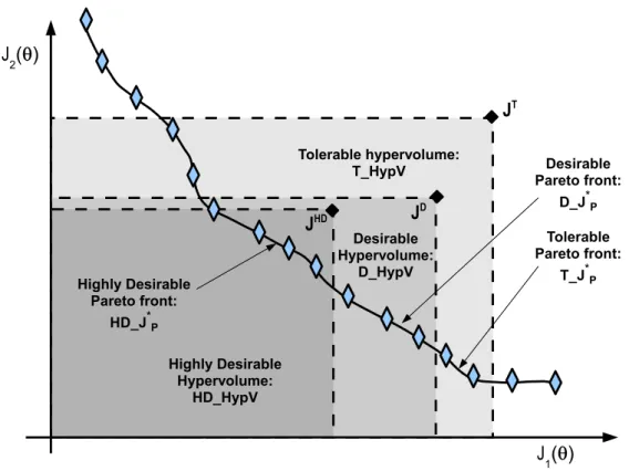
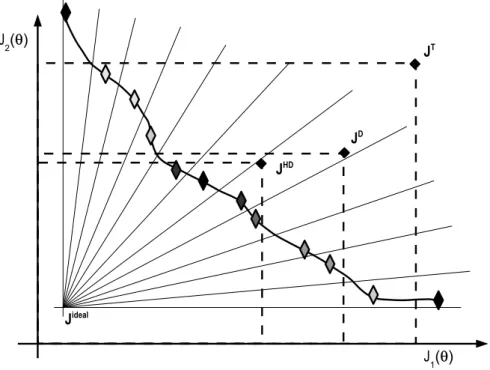
Those preference ranges are defined for the sake of flexibility (as it will be shown) to evolve the population to a pertinent Pareto front. The following definitions will be used (see Figure 7):

T Vector: JT = [J3

1, J23,· · · , Jm3], i.e. the vector with the maximum value for each

objec-tive in the tolerable range.

D Vector: JD = [J2

1, J22,· · · , Jm2],i.e. the vector with the maximum value for each

objec-tive in the desirable range.

HD Vector: JHD = [J1

1, J21,· · · , Jm1], i.e. the vector with the maximum value for each

objective in the highly desirable range.

T HypV: The hypervolume of the Pareto front approximation bounded by JT.

D Hypv: The hypervolume of the Pareto front approximation bounded byJD.

(17)

T J∗

P: the tolerable Pareto front approximation where all solutions dominate JT.

D J_P∗: the desirable Pareto front approximation where all solutions dominate JD.

HD J_P∗: the highly desirable Pareto front approximation where all solutions dominate

JHD_.

Figure 7: Graphical representation of the definitions stated.

3.2. Population selection and archive update

The Jgpp(ϕ) index will be used as a selection mechanism in the evolutionary technique.

Nevertheless, using it through the entire evolution process is not a practical approach. This is because theJgpp(ϕ) would lead the entire population to converge to a single solution, since

the physical index converges to a single Pareto optimal solution. To avoid this, a mechanism must be designed to evolve the population to a zone of interest and then encourage diversity. In this case, a switch operator is used in DE to change the selection criteria (Algorithm 5) at a certain value Jmax

gpp .

This Jmax

gpp value needs to be previously defined. This upper bound on Jgpp(ϕ) will push

the population to evolve to a desired preference region. As five preference ranges are defined, an intuitive selection of such a value isJmax

gpp =Jgpp(JT). This will guarantee the population

evolves into the feasible T HypV and then performs a selection based on dominance. The evolutionary process has a strong pressure to reach the T HypV (dominance is essential);

(18)

furthermore, it is guaranteed that only tolerable Pareto optimal solutions will be contained in J∗

P.

In the case of the archiving strategy to update A, Jgpp(ϕ) is used as a pseudo-norm

measurement to select one solution for each spherical sector (see Algorithm 6). With this,

the most preferable solution according to the set of preferences P previously defined by the

designer will be retained in each spherical sector.

1 Read generation counter G;

2 Read offspring (child population) O|_G and subpopulation (parent) S|_G;

3 for i=1:Solutions in child population do

4 Calculate the physical index J_gpp(J(ui)) and J_gpp(J(θi)); 5 if J_gpp(J(ui))> Jmax

gpp AND Jgpp(J(θi))> Jgppmax then 6 if J_gpp(J(ui))< J_gpp(J(θi))then

7 ui substitutes θi in the main population P|_G

8 end

9 end

10 if J_gpp(J(ui))< Jmax

gpp AND Jgpp(J(θi))> Jgppmax then 11 ui substitutes θi in the main population P|_G

12 end

13 if J_gpp(J(ui))< Jmax

gpp AND Jgpp(J(θi))< Jgppmax then

14 if ui θi AND θi ∈P|_G then

15 ui substitutes θi in the main population P|_G

16 end

17 end

18 end

19 Selection procedure terminates. Return parent population P|_G;

Algorithm 5: DE selection procedure with global physical programming.

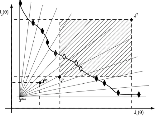
3.3. Tolerable solution handling

The previously mentioned feature could be enough if the DM is satisfied with considering solutions that might have all their individual objective values in the tolerable region (for example). Nevertheless, the DM is usually willing to accept just some of the objectives in a given region (see Figure 8). Such a feature can be incorporated into the pruning mechanism by modifying Jmax

gpp . For example, it is assumed that the DM is dealing with an m-objective

problem. The following values 10 _{could be stated for}_Jmax

gpp :

• IfJmax

gpp =Jgpp(JT), then solutions with theirmobjectives in the tolerable region might

appear inJ∗ P.

10

(19)

1 Read generation counter G; 2 Read ˆA|_G to be prune;

3 Read and update extreme values for J_ref|_G;

5 calculate its normalized spherical coordinates (Definition 3)

6 end

7 Build the spherical grid (Definitions 4 and 5);

9 calculate its spherical sector (Definition 6)

10 end 11 for i=1:SolutionsInParentPopulation do 12 if J_gpp(J(θi))> Jmax gpp then 13 θi is discarded 14 end 15 if J_gpp(J(θi))≤Jmax gpp then

16 Compare with the remaining solutions in A|_G;

17 if no other solution has the same spherical sector then

18 it goes to the archive A|_G₊₁

19 end

20 if other solutions are in the same spherical sector then

21 it goes to the archive A|_G₊₁ if it has the lowest J_gpp(J(θi))

22 end

23 end

24 end

25 Pruning ends. Return A|_G₊₁;

Algorithm 6: Spherical pruning with physical programming index.

• If Jmax gpp = Jgpp([ T olerable z }| { J₁3, J₂3, . . . , J_m3₋₁, Desirable z}|{

J_m2 ]), then solutions with their m objectives in the tolerable region will not appear in J_P∗.

• If Jmax gpp =Jgpp([ T olerable z }| { J₁3, J₂3, . . . , J_m3−2, Desirable z }| {

J_m2−1, Jm2]), then solutions with m−1 or more

objec-tives in the tolerable region will not appear inJ∗ P. • If Jmax gpp = Jgpp([ T olerable z }| { J₁3, J₂3, . . . , J_m3₋₃, Desirable z }| {

J_m2₋₂, J_m2₋₁, J_m2]), then solutions with m−2 or more objectives in the tolerable region will not appear in J∗

P.

(20)

Figure 8: Handling of tolerable solutions. The algorithm will avoid (on the designer’s request) solutions with several tolerable values (light solutions) according with theJmax

gpp value defined. In the example, bi-objective

vectors with both values in the tolerable zone are omitted.

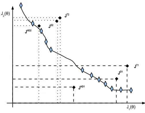
3.4. Multiple preference coding

The designer may state more than one preference setPfor a given MOP. This could be the case of a many-objective optimisation, where the DM is willing to accept some degradation in one objective, if he or she can assure outstanding performance on the remainder (see Figure 9). It is assumed that the designer defines K different preference sets; therefore, the Equation (24) is redefined as:

Jgpp(ϕ) = min k=[1,...,K] m X q=1 ηq(ϕ)|_Pk ! (25)

3.5. Pareto front approximation size control

The GPP can be used as a mechanism to dynamically adapt the algorithm according to the desired set of solutions. Instead of reducing the grid size, Jmax

gpp will be modified to retain

the most preferable solutions (Figure 10). A threshold for a desired number of solutions [car(J∗

P), car(JP∗)] will be stated. A simple dynamic adaptation of Jgppmax is described in

Algorithm 7. With this mechanism, the pruning technique will concentrate towards the HD-HypV, if the required number of solutions in the T-HypVis beyond the bound car(J∗

(21)

Figure 9: Multiple preference set definition.

1 if car(A|_G)> car(J∗

P) then

2 Sort elements on A|_G according to their J_gpp(J(θ)) index; 3 Substitute Jmax

gpp value with the physical norm of the car(JP∗)-th element; 4 Prune any element on A|_G with J_gpp(J(θ))> Jmax

gpp

5 end

6 Return A|_G;

(22)

Figure 10: Dynamic size control. Less preferable solutions are omitted (on the designer’s request) in the external archive A. The darker the solution, the more valuable according to the preference set. Extreme solutions are always preserved.

3.6. Algorithm proposal: spMODE-II.

With the aforementioned Algorithms 3, 5, 6 and 7, it is possible to re-write Algorithms 1 and 2 in order to state a proposal using GPP to improve pertinency of the J_P∗. Therefore, a preference based spherical pruning with multi-objective differential evolution algorithm (spMODE-II) preferences is presented (see Algorithm 8). Some discussions on this proposal follows below.

3.6.1. Comparison with other approaches: strengths and limitations

As commented in the introduction, the PP technique has been merged before with multi-objective optimization algorithms. For example, in [1], an aggregate multi-objective function approach was used, running several optimization statements to generate a Pareto front ap-proximation. Differences with this approach (beyond the structural differences of using a MOEA instead of a local optimisation algorithm), are related with the features commented on previously. While this algorithm does not incorporate a mechanism for multiple preference conditions or size control, the spMODE-II does.

According to the classification presented in Section 2.2, the spMODE-II algorithm uses

an a priori preference handling mechanism. Such a mechanism, based on GPP, states a

framework where dominance is essential (see Algorithm 5), and enables the algorithm to define priorities on design alternatives according to anobjective value against objective value

(23)

3 Apply dominance criterion on P|₀ to obtain A|₀; 4 while stopping criterion not satisfied do

5 Read generation count G;

6 Obtain subpopulation S|_G with solutions in P|_G and A|_G;

7 Generate offspring O|_G with S|_G using DE operators (Algorithm 3).; 8 Evaluate offspring O|_G;

9 Update population P|_G with offspring O|_G according to J_gpp(J(θ)) values

(Algorithm 5);

10 Apply dominance criterion on O|_GSA|_G to obtain ˆA|_G;

11 Apply pruning mechanism based on J_gpp(J(θ)) (Algorithm 6) to prune ˆA|_G to

obtain A|G+1;

12 Apply dynamic size control on A|_G₊₁ (Algorithm 7);

13 Update environment variables (if using a self-adaptive mechanism);

14 G=G+ 1;

15 end

P =A|G;

Algorithm 8: spMODE-II.

simultaneously (which could be helpful to deal with subset against subset priorities) and approximating Pareto optimal solutions for each of them (see Equation 25); it is indifferent to the Pareto front shape, and enables the designer to specify how many solutions are required for the MCDM step (see Algorithm 7).

Mechanisms such as goal vectors, which use one or more proposal vectors to redirect the evolution process, are similar to the spMODE-II algorithm, in the sense that dominance is

essential. Nevertheless, such vectors need to be carefully chosen. A goal vector selected

inside or outside of the Pareto front could affect the algorithm performance. The presented proposal brings the flexibility of a better redirection of the evolution process.

The proposal also assumes that the designer has an idea about the undesirability, toler-ability, or desirability for a given objective value. That may not be the case, and sometimes for the designer it is only important to prioritize some of the objectives (Objective against

objective). This is a limitation for the algorithm; therefore, in such a case, fitter mechanisms

such as the one proposed in [61] should be used.

Finally, another limitation of this approach is that it states the preferences only in an a

priori step. In the event that the designer is willing to refine a given set(s) of preferenceson

the fly (progressive scheme), then proposals such as [62] will be more appropriate for such

(24)

3.6.2. Using spMODE-II in EMO: discussions and insights

Using GPP or related approaches brings the additional task of defining K preference sets

P. Nevertheless, in several instances this supplementary effort could be justifiable if it brings a Pareto set approximation with more pertinent solutions to the DM, and so facilitating the decision making step. Therefore, the DM must be willing to spend this additional effort at the beginning of the MOP statement definition. If upper and lower bounds on objectives are known and are sufficient to improve pertinency, a simple constraint coding could be used, such as the one proposed in [4] where bounds onJ∗

P are stated.

A statement to discourage the usage of the approach presented here could be the need to define the preference set P. It is fundamental to have an understanding of the objectives to define the preference ranges. Nevertheless, if the DM has no idea about such values, it could be an indicative of a perfunctory or precipitate selection of design objectives. Therefore, perhaps the DM should ponder the design objectives stated. One of the advantages of MOEAs is the use of more interpretable and meaningful objectives for the DM and this aspect should be exploited.

Finally, according to the number of solutions, the designer could adopt a ten times the

number of objectives rule of thumb, based on [31]. In such work, it is noticed that for

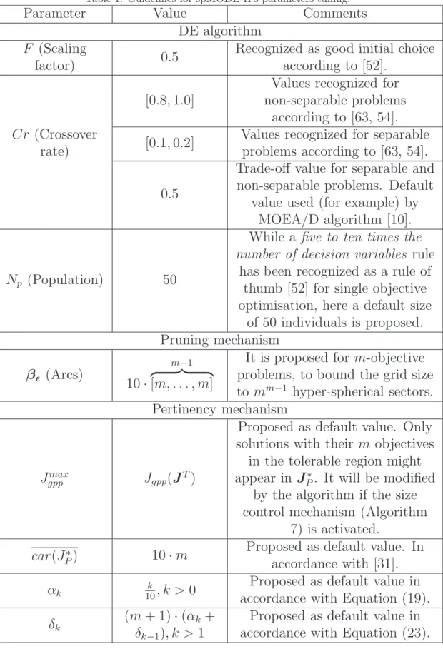
2-3 objectives a set of 20-30 design alternatives could be handled by the DM. In Table 1 guidelines for parameter adjustment of the spMODE-II algorithm are given.

4. Experimental Setup

Different tests are defined to evaluate the presented proposal. In all cases, parameters used for DE are F = 0.5 and Cr = 0.9 with an initial population of 50 individuals. The subpopulation S|G uses half of the individuals from P|G and half of the individuals from A|G. Regarding the GPP index, values αk= ₁₀k, k >0 and δk= (m+ 1)·(αk+δk−1), k >1

are used (in accordance with Table 1).

4.1. The 3-bar truss design problem

The first problem is the well-known bi-objective 3-bar truss design. The truss design problem is a classical MOP benchmark statement to test algorithms, as well as decision making step procedures. The truss parameters proposed in [48] are used. Two objectives are minimized: deflection squared (J1(θ), [cm2]) and total volume (J2(θ), [cm3]), where each

bar is constrained to a maximum stress σ < 2E+ 008 [Pa]. Characteristics to be evaluated with this benchmark problem are:

• The implicit constraint handling mechanism with Jgpp(ϕ) and the pruning technique.

• The capacity to build a T J∗

P, D JP∗ and HD JP∗ in one single run.

• Pareto front approximation control size.

As a rule of thumb, it will be stated that the DM looks for a Pareto set approximation with 10·m= 20 solutions (approximately). Preferences stated for this problem are shown in

(25)

Table 1: Guidelines for spMODE-II’s parameters tuning.

Parameter

Value

Comments

DE algorithm

F

(Scaling

factor)

0 .

5 Recognized as good initial choice

according to [52].

[0

.

8 ,

1 .

0]

Values recognized for

non-separable problems

according to [63, 54].

Cr

(Crossover

rate)

[0

.

1 ,

0 .

2]

Values recognized for separable

problems according to [63, 54].

0 .

5 Trade-off value for separable and

non-separable problems. Default

value used (for example) by

MOEA/D algorithm [10].

N

p

(Population)

50 While a

five to ten times the

number of decision variables

rule

has been recognized as a rule of

thumb [52] for single objective

optimisation, here a default size

of 50 individuals is proposed.

Pruning mechanism

β

ǫ

(Arcs)

10

·

m−1

z

}|

{

[

m, . . . , m

]

It is proposed for

m

-objective

problems, to bound the grid size

to

m

m−1

_{hyper-spherical sectors.}

Pertinency mechanism

J

max

gpp

J

gpp

(

J

T

)

Proposed as default value. Only

solutions with their

m

objectives

in the tolerable region might

appear in

J

_P∗

. It will be modified

by the algorithm if the size

control mechanism (Algorithm

7) is activated.

car

(

J

∗

P

)

10

· m

Proposed as default value. In

accordance with [31].

α

k ₁₀k

, k >

0 Proposed as default value in

accordance with Equation (19).

δ

k

(

m

+ 1)

· (

α

k

+

δ

k−1

)

, k >

1 Proposed as default value in

accordance with Equation (23).

(26)

Table 2: Preferences for the 3-bar truss design problem. Five preference ranges have been defined: highly desirable (HD), desirable (D), tolerable (T) undesirable (U) and highly undesirable (HU).

Preference Set A ← HD → ← D → ← T → ← U → ← HU → Objective J0 i Ji1 Ji2 Ji3 Ji4 Ji5 J1(θ) [cm2_] _0.00 _0.06 _0.08 _0.10 _0.20 _0.50 J2(θ) [cm3_] _0.00 ₅₅₀ ₆₅₀ ₇₅₀ ₁₀₀₀ ₁₅₀₀

G1(θ) [Pa] <2E+008 <2E+008 <2E+008 <2E+008 2E+008 2E+008

G2(θ) [Pa] <2E+008 <2E+008 <2E+008 <2E+008 2E+008 2E+008

G3(θ) [Pa] <2E+008 <2E+008 <2E+008 <2E+008 2E+008 2E+008

Table 2. Notice that constraints are incorporated as additional objectives; since the designer is just interested in calculating solutions withGi(θ)<2E+008 [Pa], no further specifications

are required below the tolerable value. These additional objectives are used to calculate the

Jgpp(ϕ) index, but they will not be used for partitioning the space, unless required.

The results of one single typical run are shown in Figure 11. The following observations can be made:

1. In Figure 11a, a typical run with a grid size of 500 spherical sectors is shown. In this case, it is important to notice that the algorithm is capable of reaching the HD J∗

P,

but using computational resources without regarding the areas of interest to the DM. 2. In Figure 11b, the algorithm is executed again, with the same parameters, but using the

Jgpp(ϕ) index. In this case, the algorithm spends resources taking care of T HypV.

3. Finally, in Figure 11c, the algorithm is executed again, with the size control mechanism. Note how the algorithm concentrates on theHD HypV, sacrificing all solutions in the

T HypV, and retaining few solutions from the desirable Pareto front.

Certainly, for bi-objective problems (most of the cases) it is not difficult to attain a Pareto front approximation such as the one in Figure 11a and apply successive filtering to reach the highly desirable region. Nevertheless, with cost function evaluations with high computational loads (complex simulations for example) it could be a desirable characteristic to evolve quickly to the desirable zone.

Usually, it is not difficult to perform an analysis on bi-objective problems, for trade-off and preference articulation. To evaluate the flexibility of the Jgpp(ϕ) index a problem with

three objectives is analysed below.

4.2. The DTLZ2 benchmark problem

The second benchmark example is the DTLZ2 problem [64], with three objectives and ten decision variables. The Pareto front is the surface contained on the first quadrant of a hypersphere with unitary radius. It is used to show the following characteristics:

(27)

0.02 0.04 0.06 0.08 0.1 0.12 0.14 400 600 800 1000 1200 1400 1600 J₁(θ) : Deflection squared [cm2] J2 ( θ ): Total Volume [cm 3] JHD JD JT

(a) No preferences used.

0.04 0.06 0.08 0.1 0.14 400 550 650 750 1600 J₁(θ) : Deflection squared [cm2] J2 ( θ ) : Total volume [cm 3] JT JD JHD

(b) GPP is used. Solutions on the tolerable hypervolume are only considered.

0.04 0.06 0.08 0.1 0.14 400 550 650 750 1,600 J 1(θ) : Deflection Squared [cm 2_] J2 ( θ ) : Total Volume [cm 3] 0.04 0.06 400 550 650 JHD JD JT JHD

(c) Size control. Original grid size is always preserved

(28)

Table 3: Preferences for the DTLZ2 benchmark problem. Five preference ranges have been defined: highly desirable (HD), desirable (D), tolerable (T) undesirable (U) and highly undesirable (HU).

Preference Set A

←

HD

→ ←

D

→ ←

T

→ ←

U

→ ←

HU

→

Objective

) [-]

0.00

0.05

0.10

0.40

1.00

10 J

2

(

θ

) [-]

0.00

0.30

0.40

0.60

1.00

10 J

3

(

θ

) [-]

0.00

0.50

0.80

0.90

1.00

10

• Capacity to build a T J∗

P, with solutions with at least one objective in the desirable

hypervolume (or equivalently, solutions with two objectives in the tolerable value). Preferences stated for this problem are shown in Table 3. Furthermore, it will be stated that the DM has some interest in keeping the objectives in the desirable zone and is willing to accept two of them (and not more) in the tolerable region; for this reason,Jmax

gpp is adapted

toJmax

gpp =Jgpp([J13, J23, J32]).

In Figure 12, results for the following algorithm executions are shown: • Execution with no preferences (∗), used for comparison purposes. • Execution to build a T J∗

P (blue circles ).

• Execution to build a T J_P∗ with at most two objectives in the tolerable zone (black diamonds ♦).

Regarding theT J∗

P, the algorithm reaches the zone according to the preferences defined

earlier. The (apparently) irregular distribution is owing to the selection of the most preferable solution inside each spherical sector. With regard to the tolerable Pareto front with at most two objectives in the tolerable region, the algorithm is capable of avoiding solutions in the middle of the tolerable region (J2(θ) ≈ [0.4,0.5]), which corresponds to solutions with Jgpp(ϕ) > Jgpp([0.4,0.6,0.8]) and consequently, uninteresting to the DM (any solution with Jgpp([0.4,0.6,0.8]) < Jgpp(ϕ) ≤ Jgpp([0.4,0.6,0.9]) has its three objectives in the tolerable

region). This fact shows the flexibility of the approach of evolving its population towards different regions of interest and avoiding regions that are uninteresting to the DM.

The flexibility in reaching regions of interest and the capacity to adapt the archive size according to the desired number of solutions, enables the algorithm to deal with many-objective optimisation. A many-many-objective problem is then used to show the ability of the approach to deal with higher dimensions.

4.3. Parametric controller tuning

The following example is a parametric controller design for the control benchmark pro-posed at the American Control Conference (ACC) [65]. The MOP statement described in

(29)

0 0.5 1 0 0.5 1 0 0.5 1 J₁(θ) J_P* J₂(θ) J3 ( θ ) 0 0.5 1 0 0.5 1 0 0.5 1 J 1(θ) J_P* vs. T_J_P* J₂(θ) J3 ( θ ) 0 0.5 1 0 0.5 1 0 0.5 1 J₁(θ) J P * vs. T_J P *

with solution handling

J₂(θ) J3 ( θ ) 0 0.05 0.1 0.15 0.2 0.25 0.3 0.35 0.4 0.2 0.3 0.4 0.5 0.6 T_J P * vs. Solution Handling J₁(θ) J2 ( θ )

Region with three objectives in the tolerable zone

Figure 12: Performance of the tolerable solution handling mechanism. Pareto front approximation (red-∗), tolerable Pareto front (blue-o) and Pareto front approximation with at most two values in the tolerable zone (black-♦) are depicted.

(30)

Table 4: Preferences for parametric controller tuning example. Five preference ranges have been defined: highly desirable (HD), desirable (D), tolerable (T) undesirable (U) and highly undesirable (HU).

Preference Set A ← HD → ← D → ← T → ← U → ← HU → Objective J0 i Ji1 Ji2 Ji3 Ji4 Ji5 J1(θ) [-] -0.01 -0.005 -0.001 -0.0005 -0.0001 0 J2(θ) [-] 0.85 0.900 1.000 1.5000 2.0000 10 J3(θ) [sec] 14.00 16.000 18.000 21.0000 25.0000 50 J4(θ) [-] 0.50 0.900 1.200 1.4000 1.5000 10 J5(θ) [-] 0.50 0.700 1.000 1.5000 2.0000 10 J6(θ) [sec] 10.00 11.000 12.000 14.0000 15.0000 50 G1(θ) [-] 2.00 2.000 2.000 2.0000 5.0000 10

[27] is used. It has six objectives: robust stability (J1(θ) [-]); maximum control effort (J2(θ)

[-]); worst case settling time (J3(θ) [sec]); noise sensitivity (J4(θ) [-]); nominal control effort

(J5(θ) [-]); and nominal settling time (J6(θ) [sec]). Additionally, a constraint on the

over-shoot in the nominal model is imposed: G1(θ)[−] < 2 . One controller structure will be

evaluated: C(s) = θ1s 2₊_θ 2s+θ3 s3₊_θ 4s2+θ5s+θ6 (26) Characteristics to be evaluated are:

• The implicit constraint handling mechanism with GPP and the pruning technique. • Capacity to build T J∗

P, D JP∗ and HD JP∗ in a many-objective optimisation

frame-work.

• Capacity for Pareto front approximation control size.

The preference set in Table 4 is used. The calculated Pareto front for reference is depicted in Figure 13 using the LD-Tool11 _{which is an application developed in Matlab c} _{for Pareto}

front visualisation using level diagrams [27]. With the LD-Tool, a color scheme can be used to depict interesting solutions for the DM according to her or his preference set definition. A geometrical remark is relevant in the figure: inJ1(θ) two different and isolated regions in

the Pareto front fulfil the designer’s preferences.

The results from Figure 13 can be compared with that of the ev-MOGA algorithm pre-sented in [27] and provided within the LD-Toolbox, where the preference set is used a

11

(31)

−0.1 −0.08 −0.06 −0.04 −0.02 0 0.5 1 1.5 2 2.5 3 3.5 4 J 1(θ) : Robust stability k ˆJ( θ ) k1 0.45 0.5 0.55 0.6 0.65 0 0.5 1 1.5 2 2.5 3 3.5 4 J

2(θ) : Maximum control effort

14 16 18 21 0 0.5 1 1.5 2 2.5 3 3.5 4 J

3(θ) : Worst case settling time

2 3 4 5 6 7 8 9 x 10−3 0 0.5 1 1.5 2 2.5 3 3.5 4 J₄(θ) : Noise sensitivity k ˆJ( θ ) k1 0.5 0.7 0 0.5 1 1.5 2 2.5 3 3.5 4

J₅(θ) : Nominal control effort

10 11 12 14 0 0.5 1 1.5 2 2.5 3 3.5 4

J₆(θ) : Nominal Settling time

HD HD HD HD HD D D D T T Most Preferable Regions HD Geometrical Remark 1

Figure 13: Visualization of the preferable Pareto front of the parametric controller tuning example using level diagrams.

posteriori. While it is possible to identify the pertinent regions in the Pareto front, many

computational resources were used in the remaining areas of the objective space. With the usage of GPP for preference articulation it is possible to focus the searching process in the area of interest. As a consequence in this case, the spMODE-II is capable of finding solu-tions in theT HypV but the ev-MOGA was not. This is due to the additional information embedded in the optimisation process provided by the DM.

4.4. Performance evaluation with other approaches

The last example is the pollution monitoring MOP stated and solved by the IBEA al-gorithm in [42]. The IBEA alal-gorithm is an indicator based MOEA [66], which uses the ǫ

indicator [67] to evolve the entire Pareto front approximation. The MOP states five objec-tives, each representing the expected information loss in five different monitoring stations.

(32)

minJ(θ) = [J1(θ), J2(θ), J3(θ), J4(θ), J5(θ)] (27) J1(θ) = −u1(θ1, θ2)−u2(θ1, θ2)−u3(θ1, θ2) + 10 (28) J2(θ) = −u1(θ1−1.2, θ2−1.5)−u2(θ1−1.2, θ2−1.5) −u3(θ1−1.2, θ2−1.5) + 10 (29) J3(θ) = −u1(θ1+ 0.3, θ2−3.0)−u2(θ1+ 0.3, θ2−3.0) −u3(θ1+ 0.3, θ2−3.0) + 10 (30) J4(θ) = −u1(θ1−1.0, θ2+ 0.5)−u2(θ1−1.0, θ2+ 0.5) −u3(θ1−1.0, θ2+ 0.5) + 10 (31) J5(θ) = −u1(θ1−0.5, θ2−1.7)−u2(θ1−0.5, θ2−1.7) −u3(θ1−0.5, θ2−1.7) + 10 (32) where: u1(θ1, θ2) = 3(1−θ1)2exp−θ 2 1−(θ2+1)2 (33) u2(θ1, θ2) = −10(θ1/4−θ31−θ25) exp−θ21−θ22 (34) u3(θ1, θ2) = 1 3exp−(θ1+ 1) 2₋_θ2 2 (35) subject to: θ1 ∈ [−4.9,3.2] (36) θ2 ∈ [−3.5,6.0] (37)

Characteristics to be evaluated are:

• The performance of the strategy with respect to state of the art techniques. • The capacity to build multiple T J∗

P, D JP∗ and HD JP∗ in many-objective

optimi-sation instances with different preference conditions. This will evaluate indirectly the capacity to deal with subset against subset priorities.

• The capacity for Pareto front approximation size control.

Two instances will be evaluated: a single physical matrix A and two simultaneous physical matrices B, and C (Table 5). In each case, 2000 function evaluations are used and 50 solutions are required by the DM inJ∗

P.

The proposal’s performance will be evaluated and compared against three different tech-niques:

(33)

• An IBEA [42] using DE algorithm (ρ = 0.05), hereafter denoted as IB-MODE. This strategy is selected because it is astate of the art technique for handling simultaneous preference conditions.

• A spMODE algorithm using the reference point based multi-objective optimization technique described in [47], hereafter denoted as RP-spMODE. This technique is se-lected because it is consistent with the spMODE algorithm structure, and it could be used as a customized norm in its pruning mechanism.

• A pure stochastic sampling approach, using the same function evaluations budget. This is used as a base test to evaluate the usability of the approaches above. This is because it has been remarked that sampling procedures could be more effective in many-objective optimization statements [43].

In the cases of IB-MODE and RP-spMODE, if they use the T Vector, D Vector

or HD Vector, they will evolve the Pareto front approximation towards the T HypV,

D HypV and HD HypV. In all cases, the comparison is performed with a priori tech-niques within the classification dominance is essential to appreciate their differences when

objective value against objective value is important for the designer. Progressive techniques

are intentionally omitted, since it is not possible to perform a fair comparison, given the structural differences regarding the input of the DM’s preferences. In the same way, tech-niques within the classificationobjective against objective are not included because they deal with a different knowledge of the DM’s preferences.

Parameters for spMODE-II, IB-MODE and RP-spMODE algorithms are stated (ac-cordingly for each case) as depicted in Table 1 for non-separable problems (F = 0.5 and

CR= 0.9). A total of 201 independent runs are carried out for all cases.

In Tables 6 and 7 the results of 201 independent runs for the best, median, worst and mean values of the achieved HD HypV,D HypV and T HypV are depicted. Statistical differences have been validated with the Wilcoxon test and Bonferroni correction at 95% significance level [68]. Regarding instance 1, none of the algorithms are capable of reaching the HD HypV; it is also evident the difference in performance between spMODE-II/IB-MODE against RP-spspMODE-II/IB-MODE/sampling approaches. The spspMODE-II/IB-MODE-II algorithm is able to achieve a better performance than IB-MODE for D HypV, at the cost of degrading the

T HypV.

Regarding instance 2, only the spMODE-II algorithm is capable of finding solutions in the HD HypV for both preference sets simultaneously. Again, spMODE-II presents the same behavior when compared with IB-MODE forD HypV and T HypV. This is due to the implicit pressure on theJgpp(θ) index to continue improving the obtained solutions from

the T HypV to theHD HypV.

Pair comparisons for 50% attainment surfaces are depicted in Figures 15 and 16 as de-scribed in [28] for MOEAs comparison in many-objective optimisation instances by means of level diagrams.12 _{Taxonomy to identify the visualisations is adopted from the same}

ref-12

(34)

Table 5: Preference Set A for Example 4. Five preference ranges have been defined: highly desirable (HD), desirable (D), tolerable (T) undesirable (U) and highly undesirable (HU).

Preference Set A

←

HD

→ ←

D

→ ←

T

→ ←

U

→ ←

HU

→

Objective

10

11

12 Preference Set B

←

HD

→ ←

D

→ ←

T

→ ←

U

→ ←

HU

→

Objective

8

9

15 Preference Set C

←

HD

→ ←

D

→ ←

T

→ ←

U

→ ←

HU

→

Objective

13

14

15

(35)

Table 6: Hypervolume achieved in 201 runs for a single physical matrix. Statistical differences (if any) according to the Wilcoxon test among spMODE-II (X), IB-MODE (†), RP-spMODE (‡), and the Sampling approach (§) are depicted for each instance.

Single Physical Matrix Preference Set A spMODE-IIX

IB-MODE† _RP-MODE‡ _Sampling§

Best 0.0000 0.0000 0.0000 0.0000 Median 0.0000 0.0000 0.0000 0.0000 HD Worst 0.0000 0.0000 0.0000 0.0000 Mean 0.0000 0.0000 0.0000 0.0000 std 0.0000 0.0000 0.0000 0.0000 Best 1.2533 0.6902 0.1291 0.3610 Median 1.1586†,‡,§ _0.6342X,‡,§ _0.0000X,† _0.0000X,† D Worst 0.5880 0.5611 0.0000 0.0000 Mean 1.1320 0.6324 0.0060 0.0197 std 0.0971 0.0219 0.0183 0.0690 Best 260.0377 259.1223 93.2508 193.5246 Median 146.6786†,‡,§ _242.2504X,‡,§ _28.1823X,†,§ _73.2174X,†,‡ T Worst 123.8105 216.6591 5.3231 1.5615 Mean 184.3619 242.0966 28.0505 75.0959 std 47.7800 7.2756 12.7703 45.1002

Table 7: Hypervolume achieved in 201 runs for simultaneous physical matrixes. Statistical differences (if any) according to the Wilcoxon test among spMODE-II (X), IB-MODE (†), RP-spMODE (‡) and the Sampling approach (§) are depicted for each instance.

Simultaneous Physical Matrixes

Preference B Preference C

spMODE-II IB-MODE RP-spMODE Sampling spMODE-II IB-MODE RP-spMODE Sampling

Best 0.1782 0.0148 0.0000 0.0331 0.3987 0.0000 0.2055 0.1256 Median 0.1241†,‡,§ _0.0000X _0.0000X _0.0000X _0.3147†,‡,§ _0.0000X,‡ _0.1331X,†,§ _0.0000X,‡ HD Worst 0.0293 0.0000 0.0000 0.0000 0.0952 0.0000 0.0002 0.0000 Mean 0.1187 0.00007 0.0000 0.0003 0.3091 0.0000 0.1279 0.0084 std 0.0308 0.0010 0.0000 0.0027 0.0550 0.0000 0.0400 0.0233 Best 56.8633 52.2928 13.3139 29.9494 123.9829 18.5836 60.0368 115.6656 Median 49.7769†,‡,§ _9.1762X,‡,§ _0.7073X,† _0.0000X,† _47.7898†,‡,§ _6.0634X,‡,§ _35.7351X,† _31.8531X,† D Worst 21.0424 0.0000 0.0000 0.0000 20.8970 0.0000 19.6379 0.0000 Mean 48.1316 8.7044 1.3396 5.6535 47.7064 5.8899 36.0081 34.6440 std 6.2359 6.6696 1.9116 7.8667 9.9826 4.6920 8.6873 24.3320

Best 515.4334 585.4359 193.5993 404.7116 1.9292E+003 1.7819E+003 1.2116E+003 1.8011E+003

Median 429.8147†,‡,§ _461.2593X,‡,§ _67.4729X,†,§ _125.5715X,†,‡ _1.3083E+003†,‡,§ _1.5312E+003X,‡,§ _0.7290E+003X,†,§ _0.9802E+003X,†,‡

T Worst 218.4111 257.7210 9.6223 0.0000 1.0425E+003 0.8677E+003 0.2501E+003 0.1507E+003

Mean 423.7853 456.3398 69.6058 141.8065 1.3138E+003 1.5044E+003 0.7350E+003 0.9970E+003

(36)

0 0.2 0.4 0.6 0.8 1 1.2 D_HypV

spMODE−II IB−MODE RP−spMODE Sampling

0 50 100 150 200 250 T_HypV

spMODE−II IB−MODE RP−spMODE Sampling 0 0.05 0.1 0.15

Preference Set B

0 10 20 30 40 50

0 100 200 300 400 500 600

spMODE−II IB−MODE RP−spMODE Sampling 0 0.1 0.2 0.3 0.4 Preference Set C

0 20 40 60 80 100 120

500 1000 1500 2000

spMODE−II IB−MODE RP−spMODE Sampling −0.5

0 0.5

HD_HypV

Preference Set A

Figure 14: Hypervolume achieved in 201 runs. Boxplot diagrams and density estimations are shown in each case.

(37)

erence13. In this visualization, any surface above 1.0 is dominated, while any surface below 1.0 dominates the other.

It is possible to notice the following remarks on Figure 15:

Remark 1: In instance 1 (single preference condition) the 50% attainment surface of the spMODE-II algorithm fails to converge at the D HypV. This impossibility is due to Objective 1: the algorithm fails to handle this objective to reach the T J∗

P. As a

consequence, the IB-MODE algorithm dominates this attainment surface portion.

Remark 2: In the same case, when the 50% attainment surface of the spMODE-II algo-rithm converges at the D HypV, it tends to dominate the IB-MODE algorithm.

Remark 3: According to instance 2 (simultaneous preference conditions), there is a change in the covering for J1(θ) and J5(θ) (Figure 15b). That could indicate structural

dif-ferences between algorithms, since one of them dominates the other in one of the objectives, at the price of being dominated in the other.

Remark 4: According to Table 7, the IB-MODE is capable of reaching the HD HypV

of the preference set B, but incapable of reaching the HD HypV of the preference set C. In Figure 15b, it is possible to appreciate this fact and it is possible to specify where it happens: in Objective J1(θ) the IB-MODE fails to reach the HD HypV of

preference set C.

Regarding Figure 16, the following remarks can be made:

Remark 5: In instance 1 (single preference condition) the 50% attainment surface of the spMODE-II algorithm consistently dominates the RP-spMODE algorithm.

Remark 6: According to Table 7, the RP-spMODE is capable of reaching theHD HypV

of the preference set C, but incapable of reaching the HD HypV of the preference set B. In Figure 16b, it is possible to appreciate this fact and it is possible to specify where it happens: in Objective J3(θ) the RP-spMODE fails to reach the HD HypV

of preference set B.

In accordance with the above, the spMODE-II algorithm shows its efficacy in handling simultaneous preference conditions to approximate pertinent Pareto front approximations for the DM.

13

LD/front/measure. For example, LD/J∗

p/kJˆ(θ)k2, means that a visual representation of Pareto front

approximationJ∗