BatchRank: A Novel Batch Mode Active Learning
Framework for Hierarchical Classification
Shayok Chakraborty
1, Vineeth Balasubramanian
2, Adepu Ravi Sankar
2,
Sethuraman Panchanathan
3and Jieping Ye
4 1Electrical and Computer Engineering, Carnegie Mellon University2Department of Computer Science and Engineering, Indian Institute of Technology, Hyderabad 3
School of Computing, Informatics and Decision Systems Engineering, Arizona State University, AZ 4Department of Computational Medicine and Bioinformatics and Department of Electrical Engineering
and Computer Science, University of Michigan, Ann Arbor
ABSTRACT
Active learning algorithms automatically identify the salient and exemplar instances from large amounts of unlabeled data and thus reduce human annotation effort in inducing a classification model. More recently, Batch Mode Active Learning (BMAL) techniques have been proposed, where a batch of data samples is selected simultaneously from an un-labeled set. Most active learning algorithms assume a flat label space, that is, they consider the class labels to be in-dependent. However, in many applications, the set of class labels are organized in a hierarchical tree structure, with the leaf nodes as outputs and the internal nodes as clusters of outputs at multiple levels of granularity. In this paper, we propose a novel BMAL algorithm (BatchRank) for hi-erarchical classification. The sample selection is posed as an NP-hard integer quadratic programming problem and a convex relaxation (based on linear programming) is derived, whose solution is further improved by an iterative truncated power method. Finally, a deterministic bound is established on the quality of the solution. Our empirical results on sev-eral challenging, real-world datasets from multiple domains, corroborate the potential of the proposed framework for real-world hierarchical classification applications.
Categories and Subject Descriptors
I.2.6 [Artificial Intelligence]: Learning; I.5.4 [Pattern Recognition]: Applications
General Terms
AlgorithmsKeywords
Active Learning, Hierarchical Classification, Optimization
Permission to make digital or hard copies of all or part of this work for personal or classroom use is granted without fee provided that copies are not made or distributed for profit or commercial advantage and that copies bear this notice and the full citation on the first page. Copyrights for components of this work owned by others than ACM must be honored. Abstracting with credit is permitted. To copy otherwise, or republish, to post on servers or to redistribute to lists, requires prior specific permission and/or a fee. Request permissions from [email protected].
KDD’15August 11 - 14, 2015, Sydney, NSW, Australia Copyright 2015 ACM ISBN 978-1-4503-3664-2/15/08 ...$15.00 DOI: http://dx.doi.org/10.1145/2783258.2783298.
1.
INTRODUCTION
Active learning algorithms have recently gained popular-ity to reduce human annotation effort in training a classifi-cation/regression model. When exposed to large amounts of unlabeled data, such algorithms automatically identify the informative samples for manual labeling. Of late, there have been research attempts towards batch mode active learning (BMAL), where a batch of unlabeled samples is selected si-multaneously for manual annotation.
Most BMAL algorithms have been developed for a flat label space, that is, they treat all the category labels inde-pendently [14, 11]. However, in many applications, the class labels are organized in the form of a tree hierarchy, where the leaf nodes contain the output classes and the internal nodes denote a super-set of the outputs at different levels of granularity. For instance, text documents are often rep-resented as a hierarchy of classes, based on their contents [16, 21]; medical images can be annotated using a class hier-archy for efficient classification [7]. Due to the tremendous increase in the generation of digital data, taxonomies and hierarchies are becoming increasing popular to adequately organize and interpret them. Thus, there is a pronounced need for an active batch selection framework in the context of hierarchical classification.
In this paper, we propose a novel BMAL algorithm, which exploits the hierarchical structure of the label tree to select the informative unlabeled samples for manual annotation. The sample selection is expressed as an NP-hard integer quadratic programming (IQP) problem. We then derive a convex relaxation, based on linear programming, and show that the batch selection task reduces to a score ranking prob-lem (hence the name BatchRank). Finally, a deterministic bound is derived on the quality of the solution, obtained using the relaxation. To the best of our knowledge, this is the first research effort to derive a concrete mathemati-cal guarantee on the solution quality of batch mode active learning in hierarchical classification. We note here that the purpose of this work is not to derive a bound on the number of queries required to achieve a given generalization error in active learning. This problem has been extensively studied in the literature [12, 1]. Our objective is to derive a math-ematical guarantee on the solution quality of the convex relaxation of BMAL in hierarchical classification, which, to the best of our knowledge, has not been addressed till date.
2.
RELATED WORK
We start with a survey of active learning in general and then present the few existing work in active learning for hierarchical classification.
Active Learning:Active learning is a well-studied prob-lem in the machine learning literature. Several techniques have been developed over the last few years and a review of these can be found in [23]. In a typical pool-based active learning setting, the learner is exposed to a pool of unla-beled samples and it iteratively selects samples for manual annotation. Pool-based active learning is further classified intosingle instance selection(where a single unlabeled sam-ple is selected in each iteration) andbatch selection (where a batch of samples is selected simultaneously and is effective in utilizing the presence of multiple labeling oracles). Since the focus of this research is on batch mode active learning (BMAL), we present existing work in this field below.
Initial BMAL techniques were largely based on extend-ing the pool-based approaches to the batch settextend-ing usextend-ing greedy heuristics [2, 22]. More recently, optimization based strategies have been proposed which have been shown to outperform the heuristic approaches. Hoi et al. [15, 13] used the Fisher information matrix as a measure of model uncertainty and proposed to query the set of points that maximally reduced the Fisher information. The same au-thors [14] proposed a BMAL scheme based on SVMs where a kernel function was first learned from a mixture of labeled and unlabeled samples, which was then used to identify the informative and diverse examples through a min-max framework. Guo and Schuurmans [11] proposed a discrimi-native strategy that selected a batch of points which maxi-mized the log-likelihoods of the selected points with respect to their optimistically assigned class labels and minimized the entropy of the unselected points in the unlabeled pool. Recently, Guo [10] proposed a batch mode active learning scheme which maximized the mutual information between the labeled and unlabeled sets and was independent of the classification model.
Active Learning in Hierarchical Classification: Ow-ing to the explosive growth in the amount of digital data, hierarchies are becoming increasingly popular to efficiently organize and categorize data. This has led to the develop-ment of several hierarchical classification algorithms. Such algorithms usually associate a vector wi with each node i
in the label tree and can be broadly categorized into two groups: recursive and non-recursive. The recursive algo-rithms start with the root node and label a data sample sequentially by selecting the category for which the associ-ated vector outputs the largest score among its siblings, until a leaf node is reached [27, 8]. Specifically, given a training set{(x1, y1),(x2, y2), . . .(xN, yN)}, a vectorwi ∈ <n is
as-sociated with each node i ∈ Y, where Y is the set of all labels in the tree. LetC(i) denote the set of all children of nodei. The recursive procedure uses classifiers f(x) that are parameterized by w1, w2, . . . wm through the following
recursive procedure: f(x) = initialize:i= 0
while C(i) is not empty
i= arg maxj∈C(i)w
T jx
returni
(1)
Non-recursive classifiers have also been proposed in the
con-text of hierarchical classification [3, 6]. A popular approach is:
f(x) = arg max
i∈Y
wiTx (2)
Even though hierarchical classification has been extensively studied, active learning in hierarchical classification is less explored. Researchers have begun to study this problem only recently (in the last 2-3 years). Liet al. [18, 19] used uncertainty sampling to select informative samples for ac-tive learning in hierarchical classification, in the context of text mining. The fundamental idea of their approach was to intelligently subdivide the unlabeled pool so as to min-imize the so-called out-of-domain queries. Cheng et al.[5] proposed a variance based uncertainty measure to query a set of informative unlabeled samples. The fundamental idea was to identify a continuous semantic space underly-ing the hierarchical structure. All the labels in the category tree were then embedded into the latent semantic space. The variance was computed by considering each label as a point and the uncertainty was computed using this variance. The same authors also introduced an active batch selection framework in the hierarchical setting using a diversity cri-terion together with the uncertainty measure [4]. To com-pute the diversity, a graph structure was used to identify the highly connected unlabeled points. A k nearest neigh-bor graph was built for every unlabeled point, which was weighted by a Gaussian kernel; the weighted matrix was used to rank all the unlabeled samples according to their diversi-ties. In each iteration, the unlabeled sample furnishing the maximum weighted uncertainty and diversity score was se-lected for manual annotation. This algorithm, Hierarchical-Structured Embedded Variance (HSEV) was shown to out-perform the previous approaches and is the state-of-the-art. Even though they exhibit good empirical performance, these techniques are heuristic in nature and also lack any quanti-tative guarantees on the solution quality.
In this paper, we present a novel batch mode active learn-ing framework for hierarchical classification. Our algorithm has a concrete mathematical foundation and also provides strong theoretical guarantees on the quality of the obtained solution. We now describe the proposed framework.
3.
PROPOSED FRAMEWORK
The recursive classifiers of the form in Equation (1) have been shown to outperform the non-recursive counterparts both in terms of accuracy and computational efficiency, in hierarchical classification [27]. We therefore use a recursive model as the underlying classifier in our framework.
3.1
Problem Set-up
Consider a batch mode active learning problem, where we are given a training setLt and an unlabeled setUt at time
t. Let wt be the classifier trained on L
t and letY denote
the set of all labels in the hierarchical label tree of depthd. The objective is to select a batch B (containingk points) fromUt in such a way that the future learnerwt+1, trained
onLtSB, has maximum generalization capability.
Batch Selection Criterion: We quantify the quality of a batch of selected samples based on their informativeness and diversity, that is, each point in the selected batch should furnish valuable information and the selected samples should have minimal redundancy among them.
Formally, we compute an information vectorc∈ <|Ut|×1 wherec(i) denotes the information furnished by the pointxi
in the unlabeled pool. The uncertainty of the trained model on a given samplexiis used as a measure of information of
that sample; higher uncertainty values denote higher degrees of information. Letyldenote the set of labels in level lof
the label tree. The uncertainty of an unlabeled samplexi
at levellis given by the entropyS(yl|xi) of the distribution
P(yl|xi), such that:
S(yl|xi) =−
X
y∈yl
P(y|xi) logP(y|xi) (3)
The posterior probability at a given node is obtained from the corresponding classification model trained at the node. The aggregate uncertainty of an unlabeled samplexiis
com-puted as the summation of the entropy values at all levels in the label tree.
c(i) =
d
X
l=1
S(yl|xi) (4)
Intuitively, the uncertainty of an unlabeled sample is com-puted as the sum of the entropy values at each level while classifying the sample using a recursive classifier.
Further, to maximize the contribution of the selected un-labeled samples, diversity based criteria have been proposed [24] which ensure that the selected samples have maximal divergence (minimal redundancy) among them. To this end, we compute a divergence matrixR∈ <|Ut|×|Ut|, whose (i, j)th
entry is a measure of redundancy between unlabeled points xiand xj (higher the value ofRij, lower the redundancy).
In our formulation, we compute the diversity between a pair of unlabeled samples as their kernelized distance. Then, the (i, j)thentry in the matrixRis given by:
R(i, j) =φ(xi, xj) (5)
Computational Considerations: Let A ∈ <n×p
de-note the matrix ofnunlabeled samples, each with dimension p. The redundancy matrixR involves computation of the pairwise distance matrixAAT, which has a complexity of O(n2p). This may be expensive (and often prohibitive) for largenandp, which are frequently encountered in modern applications.
We first note that the matrixRneeds to be computed just once in our framework. Once we have the pairwise distance matrix of all the unlabeled samples, we can keep deleting the corresponding rows and columns from the distance matrix (as batches of unlabeled samples are selected for annotation) to get an updated distance matrix for the new set of unla-beled samples. This matrix can be computed offline before the active learning iterations commence. Further, we use the concept of random projections to reduce the computa-tional overhead. Random projections have been successfully used to speed up computations, where the original data ma-trixA∈ <n×p
is multiplied by a random projection matrix X ∈ <p×d
to obtain a projected matrix B ∈ <n×d
in the lower dimensional spaced:
B=√1
dAX (6)
whered << min(n, p). X is typically populated using the entries from the standard normal distributionN(0,1), lead-ing to many well-known theoretical results [25]. In our work,
we adopt the idea ofVery Sparse Random Projections pro-posed by Liet al. [17]. The random matrixX is computed as: X(j, i) =√s 1, with prob 1 2s 0, with prob 1−1 s −1 with prob 1 2s (7)
We uses =√pto significantly speed up the computation, by a factor of √por more [17]. Let {ui}ni=1 ∈ <p denote the rows in the original data matrix A and {vi}ni=1 ∈ <d be the rows in the projected data matrixB, such thatvi=
1
√
dX T
ui. Also, letu1, u2, v1, v2denote the two leading rows
respectively. Then, it can be proved that [17]: E(||v1−v2||2
) =||u1−u2||2
(8) Very sparse random projections therefore preserve pairwise 2-norm distances in expectations while offering significant computational speed-ups. Please refer [17] for more results and detailed derivations.
Active Batch Selection Framework: By definition, all the entries inc andR are non-negative, that is,ci ≥0
andrij≥0. Also,Rii= 0,∀i. GivencandR, our objective
is to select a batch of points having high information scores and high divergence (or minimal redundancy) among them. For notational simplicity, we combinecandRinto a single matrixD∈ <|Ut|×|Ut|as follows:
D(i, j) =
(
R(i, j), ifi6=j
λc(i), ifi=j (9) where each entry in the matrix D is non-negative, that is dij ≥0,∀i, j. λis a trade-off parameter. We note that the
matrix D can be defined suitably based on the application at hand. Without any loss of generality, we proceed with the criterion based on entropy and diversity and explain our framework.
We now formulate the batch selection task as an explicit mathematical optimization problem, where the objective is to select a batch of points with high aggregate uncertainty scores and high divergences among them. Specifically, we define a binary vectormwith|Ut|entries (m∈ {0,1}|Ut|×1)
where each entrymidenotes whether the corresponding
un-labeled pointxiwill be included in the batch (mi= 1) or not
(mi = 0). Our batch selection criterion (with given batch
size k) can thus be expressed using the following integer quadratic programming (IQP) problem:
max m m T Dm s.t. mi∈ {0,1},∀i and |Ut| X i=1 mi=k (10)
The binary constraint onmi makes this IQP problem
NP-hard. We now discuss an efficient relaxation to solve this NP-hard problem1.
3.2
An Efficient Convex Relaxation
We first show that the IQP in Equation (10) is equivalent to an Integer Linear Programming (ILP) problem.
1
The problem is presumed to be NP-hard as D is just a symmetric matrix, without any other special properties. A formal proof will be taken up as part of future research.
Lemma 1. The Integer Quadratic Programming batch mode
active learning formulation in Equation (10) can be simpli-fied into an equivalent Integer Linear Programming (ILP) problem.
Proof. We introduce a binary matrix Z = (zij) with
zij = mi.mj. Thus, the optimization problem in (10)
re-duces to: max m,Z X i,j dijzij s.t. zij=mimj, |Ut| X i=1 mi=k, and mi∈ {0,1},∀i (11)
The quadratic equality constraint zij = mimj makes this
problem difficult to solve. We can show that this quadratic constraint, in fact, allows itself to be represented as a simpler linear inequality−mi−mj+ 2zij ≤0,∀i, j. This ensures
that the value ofzijis 0 if eithermiormj(or both) is equal
to 0. When bothmiandmjare equal to 1,zij is free to be
either 0 or 1. However, the maximization criterion in (11) forces the value of zij to be 1 since dij ≥ 0. Hence, the
problem can now be written as: max m,Z X i,j dijzij s.t. −mi−mj+ 2zij≤0,∀i, j and |Ut| X i=1 mi=k, mi, zij∈ {0,1},∀i, j (12)
This is an integer LP problem, proving Lemma 1. Although a global maximum exists for the ILP, it is com-putationally expensive to compute. To solve such an ILP, a standard approach is to employ the LP relaxation.
Lemma 2. The convex LP relaxation of the above ILP
(Equation 12) in Lemma1is equivalent to a ranking formu-lation based on the entries in the matrixD.
Proof. We consider the following linear program
relax-ation: max m,Z X i,j dijzij s.t. −mi−mj+ 2zij≤0,∀i, j, |Ut| X i=1 mi=k and mi, zij∈[0,1],∀i, j (13)
Since this is a maximization problem withdij≥0, at
opti-mality,zij= mi+mj
2 (from the inequality constraint−mi− mj+ 2zij≤0). Hence, (13) is equivalent to:
max m 1 2 X i,j dij(mi+mj) s.t. |Ut| X i=1 mi=k and mi∈[0,1],∀i (14)
This formulation admits an analytical (as well as an inte-ger) solution formby a simple ranking based on the entries in the matrixD. The objective in (14) can be written as
P
i,jdijmi+
P
i,jdijmj. Since the matrixDis symmetric,
the maximization problem essentially becomes equivalent to ranking the column sums ofD(hence the name BatchRank). This proves Lemma 2.
3.3
Solution Bound of BatchRank
In this section, we prove a bound on the solution to the convex LP relaxation in (14) with respect to the solution of the original NP-hard integer quadratic programming prob-lem. To this end, we transform the original maximization problem in Equation (10) into an equivalent minimization problem through the following objective function:
f(m) =||D||1−mTDm (15)
where ||D||1 = P
i,jdij. We note that since ||D||1 is
con-stant for a given matrixD, maximizingmTDmas in Equa-tion (10) is equivalent to minimizing the funcEqua-tion f(.) de-fined above, that is, maximizingmTDmand minimizingf(.) as defined above will fetch the same solution to the variable m. Since we are interested in the solution quality ofm, we prove an upper bound on the minimization problem in Equa-tion (15). Since the soluEqua-tion tomis the same, it is essentially equivalent to proving a bound on the original maximization problem in Equation (10). The main result is summarized in the following theorem:
Theorem 1. Letm∗ and mb be the optimal solutions of
the original NP-hard IQP in Equation (10) and the convex relaxation in Equation (14) respectively. Then,
f(mb)≤2f(m
∗
)
Proof. The optimization in (14) is an LP relaxation of
the quadratic formulation in (10) and thus the objective value of (14) is larger than that of (10). That is,
m∗TDm∗≤ 1 2 X i,j dij(mci+mcj) = 1 2 X i,j:mci+mdj=1 dij+ X i,j:mci+mdj=2 dij (16)
Since all entries inDare non-negative, the following holds: ||D||1=X ij dij = X i,j:mci+mdj=2 dij+ X i,j:mci+mdj=1 dij+ X i,j:mci+dmj=0 dij ≥ X i,j:mci+mdj=2 dij+ X i,j:mci+mdj=1 dij Thus, X i,j:mci+dmj=1 dij≤ ||D||1− X i,j:mci+mdj=2 dij (17)
Combining the above two, we have f(m∗) =||D||1−m∗TDm∗ ≥ ||D||1−1 2 X i,j:mci+dmj=1 dij− X i,j:mci+dmj=2 dij ≥ ||D||1−1 2 ||D||1− X i,j:mci+dmj=2 dij − X i,j:mci+dmj=2 dij = 1 2 ||D||1− X i,j:mci+dmj=2 dij = 1 2f(mb)
The first inequality follows from Equation (16) and the sec-ond from Equation (17). The last equality is true because in the evaluation ofmTDm, only the indices where bothm
i
andmjare 1 will survive, others will vanish. This completes
the proof of the theorem. We thus note that the convex re-laxation of the original NP-hard problem in BatchRank has a guaranteed bound on the solution quality.
3.4
The Iterative Truncated Power Algorithm
As evident from Lemma 2, the LP relaxation of the NP-hard IQP in Equation (10) reduces to selecting a set of k unlabeled points producing the k largest column sums of the matrixD. To further improve the solution, we use the iterative truncated-power algorithm proposed by Yuan and Zhang [26]. This solution was proposed in the context of the sparse eigenvalue problem and was also shown to be applicable to the densestk-subgraph problem (DkS). Math-ematically, DkS can be expressed as a binary quadratic pro-gramming problem, equivalent to Equation (10). Starting with an initial approximation x0, the algorithm generates a sequence of solutionsx1, x2, . . .. At each time stept, the vectorxt−1 is multiplied by the weight matrixD and then the entries are truncated to zeros except for the k largest entries, which becomes the new solutionxt. This process isrepeated until convergence. This simple, yet efficient algo-rithm has a guaranteed monotonic convergence for a positive semi-definite weight matrixD. When the matrix D is not psd, the algorithm can be run on the shifted quadratic func-tion (with a positive scalar added to the diagonal elements) to guarantee a monotonic convergence [26].
We use the BatchRank solution as the initial approxima-tionx0 followed by the iterative truncated power method to derive the final set of unlabeled samples to be selected for manual annotation. Since the convergence is monotonic, the quality of the solution can only improve over the iterations and the bound established in Theorem 1 on the quality of the solution still holds. Moreover, the running time increases only marginally due to the iterative process as it involves minimal computational overhead and converges fast. The pseudo-code for the BatchRank algorithm is given in Algo-rithm 1. The complexity of the algoAlgo-rithm isO(n2), wheren is the number of unlabeled samples.
4.
EXPERIMENTS AND RESULTS
4.1
Datasets and Experimental Setup
We used 9 datasets from different application domains, with varied feature dimensions and label tree sizes, in our
Algorithm 1BatchRank algorithm for Batch Mode Active Learning in Hierarchical Classification
Require: Training setLt, Unlabeled setUtand batch sizek
1: Train a classifierwt on the training setL t
2: Compute information vectorc(Equation 4) and the di-vergence matrixR(Equation 5)
3: Compute the matrixD, as described in Equation 9 4: Compute a vector v ∈ <|Ut|×1 containing the column
sums ofD
5: Identify theklargest entries in vand derive the initial solutionx0
6: t = 1 7: repeat
8: Computex0t=D.xt−1
9: IdentifyFtas the index set ofx 0
t with topkvalues
10: Setxt to be 1 on the index setFt and 0 otherwise
11: t = t + 1 12: untilConvergence
13: Select a batch ofkunlabeled samples based on the final solutionxt
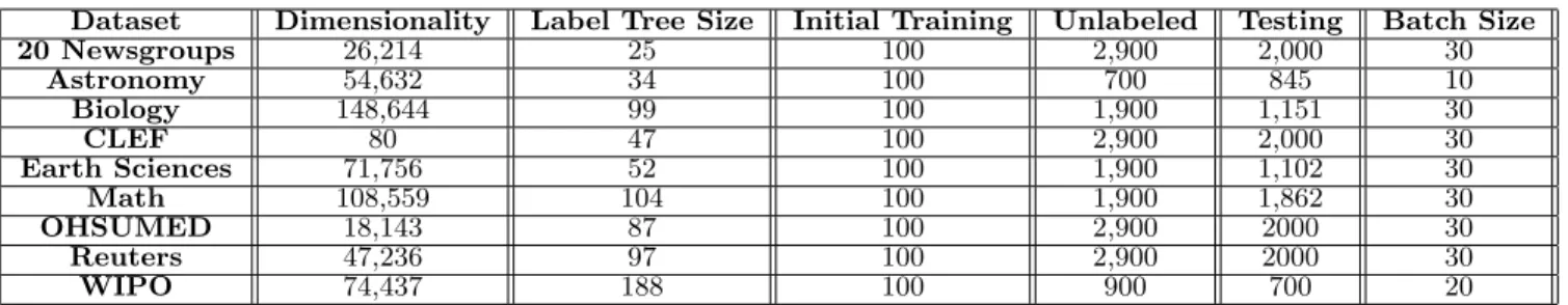
experiments, to corroborate the generalizibility of our frame-work. Each dataset was divided into an initial training set, an unlabeled set and a test set. For a given batch sizek, each algorithm selectedkinstances from the unlabeled pool to be labeled in each iteration. After each iteration, the selected points were removed from the unlabeled set, appended to the training set and the performance was evaluated on the test set. The goal was to study the improvement in perfor-mance on the test set with increasing sizes of the training set. The setup is similar to previous work [4]. All the re-sults were averaged over 5 runs, to mitigate the effects of randomness. The dataset details together with the train-ing, unlabeled and test splits are summarized in Table 1 (we only consider data samples that belong to a single leaf node in the label tree; multi-label samples, belonging to multiple leaf nodes simultaneously were discarded). The algorithms were implemented in MATLAB on an Intel Core processor with 2.60 GHz CPU and 6 GB RAM. The weight parameter λ was selected as 4 and a Gaussian kernel with parameter 1 was used to compute the kernelized distances between the unlabeled samples (based on preliminary experiments).
The entropy term in the objective function necessitates a classifier which can provide concrete posterior probability estimates of its output classes. We therefore used the hier-archical Logistic Regression (LR) as the base classification model in our experiments. As depicted in Equation (1), the hierarchical LR traverses the label tree from the root until it reaches a leaf node, and at each node, follows the child that has the largest classification score. The label at the final leaf node is the predicted label. Since most datasets used in our experiments are high dimensional and sparse (Table 1), we used the SLEP package [20] to train the models.
4.2
Competing Algorithms
We compared the proposed framework against the follow-ing three algorithms: (i)Random Sampling, where a batch of samples is queried at random (used for baseline compari-son), (ii)Uncertainty Sampling, which computes the entropy of every unlabeled sample on the leaf-node labels and the top
Dataset Dimensionality Label Tree Size Initial Training Unlabeled Testing Batch Size 20 Newsgroups 26,214 25 100 2,900 2,000 30 Astronomy 54,632 34 100 700 845 10 Biology 148,644 99 100 1,900 1,151 30 CLEF 80 47 100 2,900 2,000 30 Earth Sciences 71,756 52 100 1,900 1,102 30 Math 108,559 104 100 1,900 1,862 30 OHSUMED 18,143 87 100 2,900 2000 30 Reuters 47,236 97 100 2,900 2000 30 WIPO 74,437 188 100 900 700 20
Table 1: Dataset Details
k uncertain points are queried for annotation (k being the batch size) [5] and (iii) Hierarchical-Structured Embedded Variance (HSEV) (proposed by Chenget al. [4]), which uses an uncertainty and diversity based criterion for sample se-lection and is the state-of-the-art for BMAL in hierarchical classification. However, the HSEV is based on a heuristic sample selection strategy, where at every iteration, the un-labeled sample with the maximum weighted sum of uncer-tainty and diversity values is selected for annotation. Our method, on the other hand, is based on a concrete mathe-matical formulation and also provides theoretical guarantees on the quality of the solution.
4.3
Evaluation Metrics
We used the zero-one error (error rate) and the tree-loss error (the graph distance between the predicted and ac-tual categories) to study the performance of the algorithms. These are commonly used evaluation metrics in hierarchical classification [27].
4.4
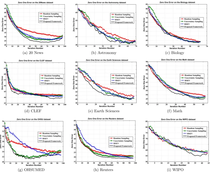
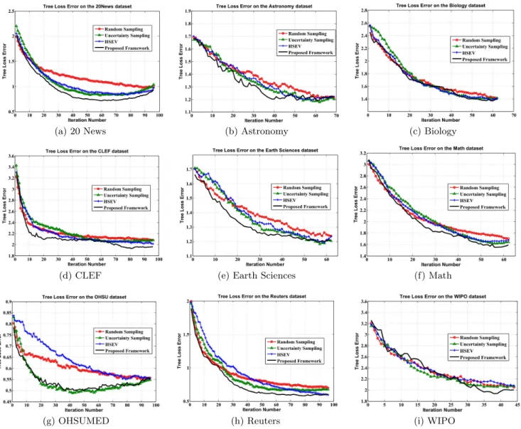
Active Learning Performance
The results are depicted in Figure 1 (0/1 error) and Fig-ure 2 (tree-loss error). In each graph, the x-axis denotes the number of iterations (rounds of active learning) and the y-axis denotes the error (0/1 or tree-loss). The pro-posed framework outperforms Random Sampling on all the datasets; both the zero-one error and the tree loss error drop at a faster rate with increasing size of the labeled set. The BatchRank algorithm therefore identifies the salient and ex-emplar instances for manual annotation and attains a given level of performance with much reduced human labeling ef-fort. The Uncertainty Sampling and HSEV methods depict better performance than Random Sampling, but are not as good as BatchRank. The proposed framework depicts the best performance in terms of both the evaluation metrics. The results unanimously lead to the conclusion that our algorithm outperforms HSEV and the other baselines con-sistently across all datasets. For the Biology and WIPO, however, the performance of all the algorithms are close.
We conducted a 2-sided paired t-test at the significance level ofp < 0.05, to compare the performance of the pro-posed BatchRank algorithm against its closest competitor across all datasets (such a test has been previously used to analyze the performance of active learning algorithms [10]). Our analysis revealed that the proposed framework outper-forms its closest competitor on 8 out of the 9 datasets used in our study (except the OHSUMED dataset). The per-formance improvement achieved by BatchRank is therefore statistically significant.
Dataset Uncertain HSEV BatchRank 20 News 2.82±1.83 3.37±2.03 5.93±1.87 Astronomy 0.90±0.57 1.17±0.71 3.77±0.82 Biology 9.80±2.62 19.32±2.08 27.78±4.87 CLEF 0.84±0.61 1.22±0.79 3.56±1.07 Sciences 3.13±1.19 6.32±2.78 7.47±2.26 Math 8.56±2.27 15.90±3.16 17.28±3.11 Ohsumed 3.79±2.31 6.06±3.66 9.28±2.94 Reuters 5.72±3.83 12.75±3.92 16.23±3.36 WIPO 3.17±2.07 13.56±3.59 19.22±3.89
Table 2: Average time taken (in seconds) to query a batch of samples from the unlabeled set.
4.5
Computation Time Analysis
In this section, we study the computation time of the BMAL algorithms. Random Sampling does not take any time practically, since it does not involve any computations; we hence exclude it from our analysis. For the proposed BatchRank algorithm, a pairwise distance matrix needs to be computed, as detailed in Section 3.1. This needs to be computed just once and can be done offline before the ac-tive learning process starts and the selected unlabeled data samples are passed to the human annotators for labeling. We therefore do not include the time taken for the distance matrix computation in our run-time analysis.
Table 2 reports the average time taken to query a batch of samples by each algorithm. The Entropy method is the most efficient in terms of computation; however, it is not consistent in its performance, as noted in Figures 1 and 2. The proposed framework depicts comparable run-time as the HSEV method. Our method, therefore, outperforms the HSEV algorithm in terms of learning performance and incurs only marginal increment in computational overhead.
4.6
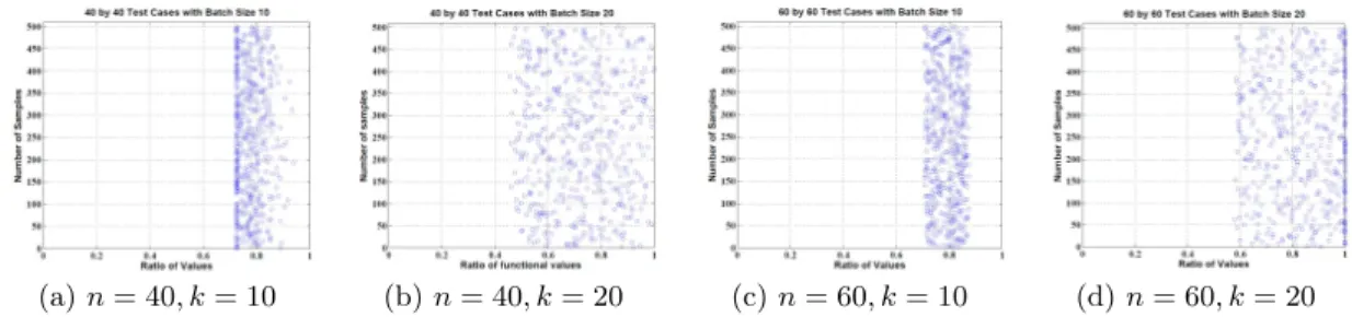
Solution Quality Analysis
In this section, we empirically validate the quality of the solution obtained using the proposed algorithm, for different values of the number of unlabeled samplesnand the batch sizek. We plot the ratio mb
TD
b
m
m∗TDm∗, wheremb is the solution
obtained using the BatchRank framework (together with the truncated power iterations) andm∗is the optimal solution (note that the IQP in Equation (10) can be solved exactly for small scale problems, which gives us the optimal solution). We present results for n = 40,60 andk = 10,20, for each value of n, in Figure 3. Each figure depicts the results of 500 random, symmetric matrices for the specific n and k. We note that the ratio of the functional values obtained using our method is very close to 1 (greater than 0.8 in most cases). This corroborates the fact that the proposed framework yields high quality approximations of the
NP-(a) 20 News (b) Astronomy (c) Biology
(d) CLEF (e) Earth Sciences (f) Math
(g) OHSUMED (h) Reuters (i) WIPO
Figure 1: BMAL for Hierarchical Classification - Zero One Error Graphs (Best viewed in color.)
hard IQP (Equation (10)) and the solutions obtained very closely match the optimal.
4.7
Parameter Sensitivity
In this section, we study the effect of batch size (number of samples selected in each iteration of active learning) and the size of the initial training set, on the learning performance. We used the 20 Newsgroups dataset for this study and the zero-one error was used as the evaluation metric. To study the effect of batch size, we used the same training, unlabeled and test splits, as outlined in Table 1. Four different batch sizes were studied - 10,30,50 and 100. The results are pre-sented in Figure 4; the proposed algorithm depicts the best performance across all batch sizes.
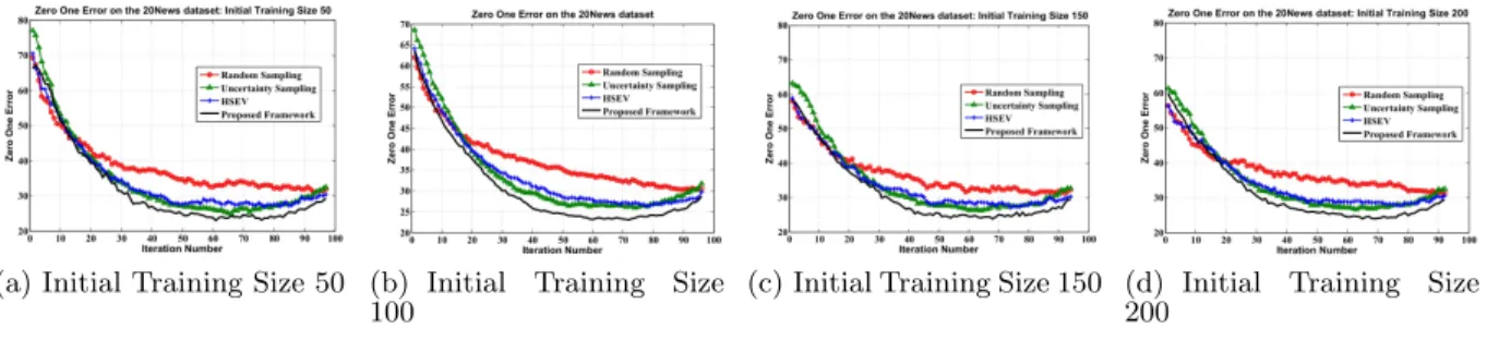
We used the following four values of the initial training set to study its effect: 50,100,150 and 200. The sizes of the unlabeled and test sets were the same as in Table 1. The batch size was fixed at 30. The results are shown in Figure 5. From the results, we conclude that the proposed framework outperforms the other algorithms consistently.
5.
CONCLUSION AND FUTURE WORK
In this paper, we proposed a novel BMAL algorithm for multi-class hierarchical classification. The selective sam-pling problem was posed as an NP-hard integer quadratic programming; we then derived a convex relaxation to solve the NP-hard IQP and established a bound on the solution quality of the relaxation. Our empirical results on several challenging, real-world datasets corroborate the merit of the proposed approach over the state-of-the-art techniques and also the fact that it delivers high quality solutions. Future work will mainly involve extension of our framework to hi-erarchical, multi-label active learning.
6.
ACKNOWLEDGMENT
This research is sponsored in part by NIH LM010730 and ONR N00014-11-1-0108.
7.
REFERENCES
[1] M. Balcan, S. Hanneke, and J. Vaughan. The true sample complexity of active learning. InMachine Learning, 2010.
(a) 20 News (b) Astronomy (c) Biology
(d) CLEF (e) Earth Sciences (f) Math
(g) OHSUMED (h) Reuters (i) WIPO
Figure 2: BMAL for Hierarchical Classification - Tree Loss Error Graphs (Best viewed in color)
[2] K. Brinker. Incorporating diversity in active learning with support vector machines.ICML, 2003.
[3] L. Cai and T. Hofmann. Hierarchical document categorization with support vector machines. InCIKM, 2004.
[4] Y. Cheng, Z. Chen, H. Fei, F. Wang, and A. Choudhary. Batch mode active learning with hierarchical-structured embedded variance. InSDM, 2014.
[5] Y. Cheng, K. Zhang, Y. Xie, A. Agarwal, and A. Choudhary. On active learning in hierarchical classification. InCIKM, 2012.
[6] O. Dekel, J. Keshet, and Y. Singer. Large margin hierarchical classification. InICML, 2004.
[7] I. Dimitrovski, D. Kocev, S. Loskovska, and S. Dzeroski. Hierchical annotation of medical images. InInternational Multiconference - Information Society IS, 2008.
[8] S. Dumais and T. Chen. Hierarchical classification of web content. InProceedings of SIGIR, 2000.
[9] M. Goemans and D. Williamson. Improved approximation algorithms for maximum cut and satisfiability problems using semidefinite programming. InJournal of the ACM, 1995.
[10] Y. Guo. Active instance sampling via matrix partition. In
NIPS, 2010.
[11] Y. Guo and D. Schuurmans. Discriminative batch mode active learning. InNIPS, 2007.
[12] S. Hanneke. A bound on the label complexity of agnostic active learning. InICML, 2007.
[13] S. Hoi, R. Jin, and M. Lyu. Batch mode active learning with applications to text categorization and image retrieval.
IEEE TKDE, 2009.
[14] S. Hoi, R. Jin, J. Zhu, and M. Lyu. Semi-supervised SVM batch mode active learning for image retrieval. InCVPR, 2008.
[15] S. C. H. Hoi, R. Jin, and M. R. Lyu. Large-scale text categorization by batch mode active learning. InWWW. ACM, 2006.
[16] D. Lewis, Y. Yang, T. Rose, and F. Li. RCV1: A new benchmark collection for text categorization research. In
JMLR, 2004.
[17] P. Li, T. Hastie, and K. Church. Very sparse random projections. InKDD, 2006.
[18] X. Li, D. Kuang, and C. Ling. Active learning for hierarchical text classification. InPAKDD, 2012. [19] X. Li, C. Ling, and H. Wang. Effective top-down active
(a)n= 40, k= 10 (b)n= 40, k= 20 (c)n= 60, k= 10 (d)n= 60, k= 20
Figure 3: Analysis of Solution Quality of the Proposed Framework
(a) Batch Size 10 (b) Batch Size 30 (c) Batch Size 50 (d) Batch Size 100
Figure 4: Effect of Batch Size on the 20 Newsgroups dataset - Zero One Error Graphs (Best viewed in color)
2013.
[20] J. Liu, S. Ji, and J. Ye. SLEP: Sparse learning with efficient projections. InTechnical Report, Arizona State University, 2009.
[21] J. Rousu, C. Saunders, S. Szedmak, and J. Shawe-Taylor. Kernel–based learning of hierarchical multilabel
classification models. InJMLR, 2006.
[22] G. Schohn and D. Cohn. Less is more: Active learning with support vector machines. InICML, 2000.
[23] B. Settles. Active learning literature survey. InTechnical Report 1648, University of Wisconsin-Madison, 2010. [24] D. Shen, J. Zhang, J. Su, G. Zhou, and C. Tan.
Multi-criteria-based active learning for named entity recognition. InACL, 2004.
[25] S. Vempala. The random projection method. InAmerical Mathematical Society, 2004.
[26] X. Yuan and T. Zhang. Truncated power method for sparse eigenvalue problems. InJMLR, 2013.
[27] D. Zhou, L. Xiao, and M. Wu. Hierarchical classification via orthogonal transfer. InICML, 2011.
APPENDIX
A.
AN IMPROVED BOUND ON THE
SOLU-TION QUALITY
In section 3.3, we derived a deterministic bound on the solution quality of the BatchRank algorithm. In this section, we attempt to improve the guarantee on the solution quality. To this end, we present a second convex relaxation to solve the original NP-hard IQP. Starting with Equation (10), we first make the following variable transformation:
yi= 2(mi− 1 2)⇒mi= yi+ 1 2 ⇒ n X i=1 yi= 2 n X i=1 mi−n= 2k−n,p
where n = |Ut| is the number of unlabeled data samples
in the unlabeled pool. The entire optimization problem in Equation (10) is now rewritten in terms of the new variable
y(ignoring the constant 14): max y X i,j dij(yi+ 1)(yj+ 1) s.t. yi∈ {−1,1},∀i and |Ut| X i=1 yi=p (18)
A.1
Multi-dimensional Relaxation
Since solving the integer quadratic program in Equation (18) is NP hard, we consider relaxations of the constraints. Specifically, we follow the strategy proposed by Goemans and Williamson [9], where each variable yi is relaxed to
a multidimensional vector vi belonging to <n of unit
Eu-clidean norm, instead of a one dimensional scalar variable. In other words, we assume that each vector vi belongs to
then-dimensional unit sphereSn. The relaxation of the NP
hard problem in Equation (18) is therefore given by (ignor-ing the constant 1):
max v X i,j dij(vTivj+v0Tvi+vT0vj) (19) s.t. vi∈Sn,∀i and |Ut| X i=1 vi=p (20)
wherev0 is a vector ofn-dimensions with all entries 1. (The equality constraint in Equation (20) implies that the sum across all the entries in all the vi vectors should equal the
scalar constantp. This is because each scalar variableyiwas
relaxed into a vector variable vi and the sum of allyi was
constrained to be equal to p). Once we solve for the vec-torsvfrom this formulation (we present the solution details below), we select a random unit vector r that is uniformly distributed on the unit sphere and find the dot product of r with every vectorvi. We then select the set of unlabeled
(a) Initial Training Size 50 (b) Initial Training Size 100
(c) Initial Training Size 150 (d) Initial Training Size 200
Figure 5: Effect of Initial Training Set Size on the 20 Newsgroups dataset - Zero One Error Graphs (Best viewed in color)
product with the random unit vectorr, as in [9]. However, we note that the number of positive dot products may not exactly equalk, which means that the number of instances selected by this algorithm may not equal the pre-specified batch size.
A.2
Semi-Definite Programming (SDP)
Relax-ation
Using the decompositionQ=BTB, we note that any pos-itive semi-definite (psd) matrix with diagonal entries 1 corre-sponds to a set of unit vectorsviif we correspond the vector
vi to the ith column of the matrix B. Then, qij = vivj,
which accounts for the termviTvj in the objective function
of Equation (19). However, to incorporate the termsvT0vi
andvT
0vj in the objective, the matrixQis decomposed as
Q= vT 0 BT v0 B
whereB= [v1v2 . . . vn]. We can therefore rewrite the entire
relaxation in terms of the defined matrixQ(in the previous equation) as follows: max Q X i,j di,j(Qi+1,j+1+Q1,i+1+Q1,j+1) (21) s.t. Qii= 1,for i = 2 to n+1, n+1 X j=2 Q1j=p, Q11=n and Q0 (Q is psd)
This is a semi-definite programming (SDP) problem and can be solved using existing software packages like SeDuMi.
A.3
Probabilistic Solution Guarantee
We first rewrite the objective in Equation (19) in a sim-plified form as follows:
X i,j dij(viTvj+vT0vi+v0Tvj) = X i,j c dij(viTvj)
where v0 is the vector obtained from the first row of the decomposed matrix after solving the SDP problem anddcij
is obtained from dij, to simplify the representation. The
main result regarding the solution bound of this algorithm is summarized in the following theorem:
Theorem 2. LetW denote the value of the objective func-tion produced using the algorithm andE(W) denote its ex-pectation. Also, letDbtotal denote the sum of all entries in
the matrixDb. Then,the following bound holds:
[E(W) +Dbtotal]≥0.87856 " X i,j c dijvivj+Dbtotal #
Proof. Consider a random unit vector r. By the
lin-earity of expectation, the expectation of the value of the objective function is given by (we drop the sub-scriptsiand jfrom the summation for notational convenience):
E(W) =Xdbij[1.P r(sgn(vi.r) =sgn(vj.r)) + (−1).P r(sgn(vi.r)6=sgn(vj.r))] =Xdbij[1−2.P r(sgn(vi.r)6=sgn(vj.r))] =Xdbij 1−2arccos(vi.vj) π
where sgn(x) = 1 if x ≥ 0 and −1 otherwise. The last equality follows from the result proved by Goemans and Williamson [9]. Further, it can be shown that for −1 ≤ z≤1, 1−arccosπ (z) ≥α.12(1 +z), where α= min 0≤θ≤π 2 π. θ 1−cosθ ≥0.87856
(the proof of the above inequality can be found in [9]). That is, 1−2arccosπ(z) ≥α(1+z)−1. Since in our formulation, the visare all unit vectors, we have−1≤z =vivj≤1, ∀i, j.
Therefore, 1−2arccos(vivj)
π ≥α(1 +vivj)−1.
Combining all of the above, we get E(W)≥Xdbij[α(1 +vivj)−1] =αXdbijvivj+ (α−1)Dbtotal ⇒[E(W) +Dbtotal]≥α " X i,j b dijvivj+Dbtotal #
which proves the theorem.
This relaxation therefore provides a better guarantee on the quality of the solution. However, this method involves solving an SDP problem, which is computationally more ex-pensive than the previous approach. Also, the number of selected samples may not exactly equal the batch size. A thorough investigation of this solution methodology will be taken up as part of future research.