MASTER THESIS
Mr./Mrs. Mohammad Mohammadi
Hankel matrices for use in
Learning Vector Quantization
Faculty of Applied Computer and Life Sciences
MASTER THESIS
Hankel matrices for use in
Learning Vector Quantization
Author: Mohammad Mohammadi Study Programme: Applied Mathematics in Digital Media Seminar Group: MA14w1-M First Referee: Thomas Villmann Second Referee: Michael Biehl Mittweida, September 2016
Bibliographic Information
Mohammadi, Mohammad: Hankel matrices for use in Learning Vector Quantization, 47 pages, 3 figures, Hochschule Mittweida, University of Applied Sciences, Faculty of Applied Computer and Life Sciences
Master Thesis, 2016
Abstract
Classification of time series has received an important amount of interest over the past years due to many real-life applications, such as environmental modeling, speech recognition, and computer vision.
In my thesis, I focus on classification of time series by LVQ classifiers. To learn a classifiers, we need a training set. In our case, every data point in the training set contains a sequence (an ordered set) of feature vectors. Thus, the first task is to construct a new feature vector (or matrix) for each sequence.
Inspired by [2], I use Hankel matrices to construct the new feature vectors. This choice comes from a basic assumption that each time series is generated by a single or a set of unknown Linear Time Invariant (LTI) systems.
After generating new feature vectors by Hankel matrices, I use two approaches to learn a classifier: Generalized Learning Vector Quntization (GLVQ) and Median variant of Generalized Learning Vector Quantization (mGLVQ).
I
I. Contents
Contents. . . I List of Figures. . . II List of Tables. . . III Preface. . . IV
1 Introduction. . . 1
1.1 Dynamical Systems. . . 2
1.1.1 Linear Time Invariant (LTI) Systems. . . 2
1.1.2 Hankel Matrix. . . 3
1.2 Principal Component Analysis (PCA). . . 4
1.3 Optimization Approaches for functionals. . . 5
1.3.1 Stochastic Gradient Descent . . . 5
1.3.2 Expectation Maximization (EM). . . 6
How the EM algorithm works. . . 6
Why the EM algorithm works. . . 8
The Generalized Expectation Maximization . . . 9
2 The Learning Vector Quantization (LVQ) for Prototype Based Classification . . . 11
2.1 Generalized Learning Vector Quantization. . . 11
2.2 The Median Generalized Learning Vector Quantization (mGLVQ). . . 13
2.2.1 Median GLVQ. . . 13
3 Using Dynamic Subspace Angles. . . 17
3.1 Principal Component Analysis for Noise Reduction. . . 17
3.2 Similarity Measures of Linear Subspaces. . . 17
3.2.1 Canonical Correlation. . . 18
3.2.2 How to compute the canonical correlation?. . . 18
3.2.3 Martin Distance [25]. . . 18
3.2.4 Alternative Dissimilarities. . . 19
3.3 Training in LVQ using Matrix based on subspace dissimiliarities. . . 19
I
Prediction. . . 20
3.3.2 Training Procedure for GLVQ usingd1(3.5), d2(3.6). . . 21
Derivative ofd1 (3.5) . . . 21 Derivative ofd2 (3.6) . . . 21 Training Procedure. . . 22 Prediction. . . 23 4 Clustering . . . 25 4.1 Neural Gas (NG). . . 25
4.1.1 The Neural Gas for matrices . . . 26
4.2 The Median Neural Gas (mNG). . . 27
4.2.1 Algorithm . . . 28 4.2.2 Convergence . . . 28 4.3 Median k-means . . . 29 5 Set of Hanklets . . . 31 5.1 Pre-processing . . . 31 5.2 Clustering Hanklets. . . 32 5.3 Labeling Hanklets. . . 32 5.3.1 Bayes’ Classifier. . . 32
5.3.2 Bayes’ Classifier for Hanklets. . . 33
5.4 Bag-of-Hanklets. . . 34
5.5 Classification Algorithm . . . 34
6 Experiments. . . 37
6.1 Algorithms in Chapter 3. . . 37
6.1.1 PenDigit Dataset (UCI) . . . 37
mGLVQ with CC . . . 37
GLVQ. . . 38
Conclusions. . . 38
6.1.2 Libras Dataset (UCI) . . . 40
mGLVQ (CC). . . 40
GLVQ. . . 40
I
6.1.3 Comparison . . . 42 7 Discussion. . . 43 Bibliography. . . 45
II
II. List of Figures
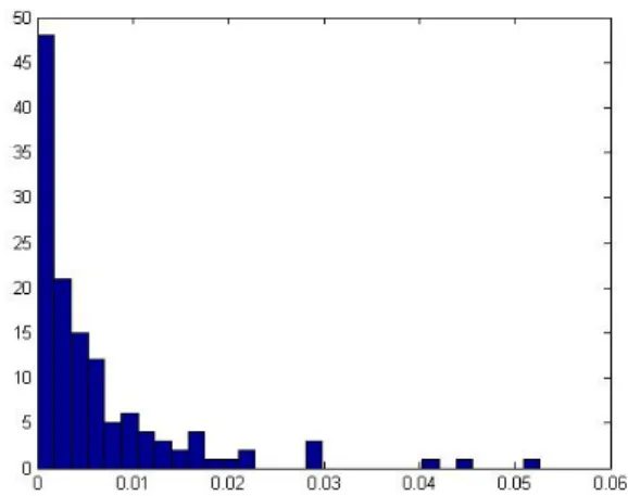
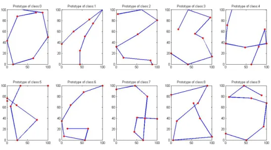
5.1 The histogram of dissimilarity scores for a typical cluster in the dictionary of Han-kelets resembles a Gamma distribution. . . 33 6.1 A data point with label 2. . . 38 6.2 Prototypes of Pendigit dataset: mGLVQ with 1 prototype per class. . . 38
III
III. List of Tables
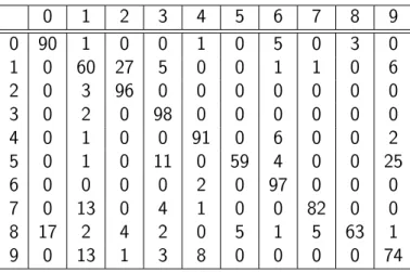
6.1 Confusion matrix of Pendigit Dataset: mGLVQ with 1 prototype per class. . . 39
6.2 Confusion matrix of Pendigit Dataset: GLVQ with 1 prototype per class. . . 39
6.3 Number of prototypes per class. . . 39
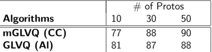
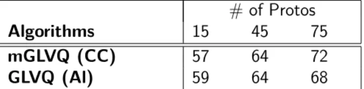
6.4 Accuracy of algorithms for PenDigit dataset. . . 40
6.5 Confusion Matrix of Libras Dataset: mGLVQ with 1 proto. . . 41
6.6 Confusion Matrix (percentage) of Libras Dataset: GLVQ with 1 proto . . . 41
IV
IV. Preface
Classification is one of the most important tasks in machine learning. The goal is to learn a classifier from a training set. There are different types of classifiers. However, my thesis focuses on learning vector quantization (LVQ) classifiers, introduced by T. KOHONEN, as one the most intuitive prototype based classification models. In [21], you can find the developments of LVQ-variants for classification tasks in relation to several aspects of classification learning.
In a training set, a data point includes a feature vector and a label. The feature vector of the data point is supposed to be fixed. However, there are some situations that the feature vector of the data point changes during the time. It means there exists an ordered set (or time series) of feature vectors for each data point. Thus, we cannot use the methods described in [21].
To be able to use LVQ methods, we need to convert a set of feature vectors to one feature vector (or matrix). Inspired by Li [2], I use Hankel matrices to construct feature matrices, and then I will use LVQ to learn a classifier.
In chapter 1, I explained why Hankel matrices are used to construct feature vectors and then how to remove noise from the feature vectors. At last, I described two optimization approaches used in LVQ to find the best values of parameters.
In chapter 2, I presented two LVQ methods for classification. At first, I explained Generalized learning vector quantization (GLVQ) introduced by Sato and Yamada[22]. Then, I described the median variant of GLVQ which is introduced by D. Nebel[12].
In chapter 3, I combined the topics in chapter 1 and 2. From chapter 1, I can construct feature vectors, and then I can use the classification approaches, explained in chapter 2, to learn a classifier. In this chapter, I proposed two procedures for classification task.
In chapter 4, I illustrated three clustering approaches: Neural Gas, median variant Neural Gas and a median variant of k-means.
In chapter 5, I described a classification algorithm. I used Bag-of-Words (BoW) models to generate feature vectors called Bag-of-Hanklets (BoHk), then I used GLVQ to learn a classifier.
In chapter 6, I presented some results from implementation. I applied the algorithms, presented in chapter 3, for two data sets: Pen Digits and Libras.
At last, I would like to express my gratitude to my supervisor Professor Thomas Villmann, for his continued and valuable mentorship and Professor Michael Biehl, for the interesting topic. I am also grateful to the members of Computational Intelligence Group, specially David Nebel. A very special thanks goes out to my dear family and friends for their moral support.
Chapter 1: Introduction 1
1
Introduction
In machine learning, classification is the problem of identifying to which of a set of categories (sub-populations) a new observation belongs. Our prediction about a new observation is based on a training set of data containing observations (or instances) whose category membership is known.
In a typical classification problem, each observation in a training set has two parts
(xi, li) (1.1)
where
• xi : a feature vector
• li : a label
However, I suppose the classification task for time series. It means each data point, instead of a single feature vector, includes an ordered set of feature vectors
(Xi, li) (1.2)
where
• Xi= (x0, x1, ..., xT) : an ordered set of feature vectors (time series)
• li : a label
Actually, this set of feature vectors represents a feature vector in which it changes during the time.
Hence, in order to classify a time series correctly, we have to discover the essence of the changes in the feature vector. So, we need a way to capture the temporal informa-tion of a time series.
Two important factors that have effect on the accuracy of prediction are: 1. The feature vectors that we use to classify
2. The dissimilarity measure to know the distance between feature vectors According to them, there are two ways to capture temporal information:
• Some works use metrics for learning of temporal information: A new metric is presented in [10]. [9] uses Sobolev metrics.
• Another way is to use appropriate feature vectors. In my thesis I will use Hankel matrix to construct new feature vectors.
In the following sections, I will explain some introductions. In the first section, I will present the definition of Linear Time Invariant (LTI) systems, and then I will use it to explain why Hankel matrices are useful. In the second section, I will describe Principal Component Analysis (PCA) which is applicable to remove noise. In the last section, I will describe two optimization strategies which are so popular.
2 Chapter 1: Introduction
1.1 Dynamical Systems
Dynamical systems are powerful tools to work with temporally ordered sets because they can capture the essence of the temporal evolution of the time series.
In a dynamical system, there are two kinds of vectors:
• State vector: It is the input vector to the system, and it represent the internal state of the system. In our case, we suppose that we do not know anything about it.
• Measurement vector: It is the output vector of the system. In our case, it is the only thing we know about system, and according to the applications it represents different things. For example, it can be the coordinate of a tracked target at time
k, or the pixel values of an images at time k.
As mentioned in [2], the goal of dynamical systems is to model temporal information of a sequence of a measurement vector yk ∈Rn, as a function of a relatively low
dimensional state vectorxk∈Rd that changes over time.
1.1.1 Linear Time Invariant (LTI) Systems
The simplest dynamical model is a linear time invariant (LTI) system.
Definition 1.1 A linear time invariant system is defined by two linear equations:
xk=Axk−1 x0 given yk=Cxk+wk
where matrices A and C are constant over time, and wherewk is uncorrelated zero mean Gaussian measurement noise.
The first equation is known as the state equation and involves the variable xk ∈ Rd, which represents the d-dimensional internal state of the LTI system. The second
equation is known as the measurement equation and provides a link between the state of the systemxk and the n-dimensional observable measurement yk.
Remark 1.2 In my thesis, I assume that
• Each time series is an output of a LTI system, and
• Time series in the same classes come from the same dynamical systems. Hence, to classify a time series, we need to find out:
• Which dynamical system could generate the time series?
To answer this question, we need a method to specify systems. One way is to estimate the dimension and values of the matricesA and C and the initial vector x0. However,
given a finite number of measurements of yk, the set of (A, C, x0) that could have
generated this data is not unique, and trying to jointly identify the dynamics(A, C)and
x0 leads to computationally challenging non-convex optimization problems [30].
Chapter 1: Introduction 3
1.1.2 Hankel Matrix
Definition 1.3 Given a sequence of output measurement vectors from the system,
y0, y1, ..., yT, its associated (block) Hankel matrixHy is:
Hy= y0 y1 y2 · · · ym y1 y2 y3 · · · ym+1 y2 y3 y4 · · · ym+2 .. . ... ... . .. ... yk yk+1 yk+2 · · · yT
wherek is the maximal order of the system. T is the temporal length of the sequence, and it holds that T =k+m−1.
Note that the columns of the Hankel matrix correspond to overlapping subsequences of the data, shifted by one time point, and that the block anti-diagonals of the matrix are constant. The following theorem [2] represents that this special structure of the matrix encapsulates the dynamic information of the system.
Theorem 1.4 Let {yk}k and {zk}k be two trajectories of a system. The columns of
two Hankel matrices Hy and Hz, corresponding to {yk}k and {zk}k, span the same
linear subspace, in the absence of noise.
Proof: Let wk≡0. According to the definition of LTI systems, we can write:
yk=Cxk=CAxk−1=CA2xk−2=...=CAkx0 (1.3)
So, the Hankel matrix can be represented as:
Hy= ΓX (1.4) where Γ = C CA .. . CAk and X=hx0 x1 · · · xm i
From the above formula, we get if the ranks of A and C are d,
f:Rd→Rkn×d
xi→Γxi
4 Chapter 1: Introduction
Rkn×d such that the dimension of this subspace is also d.
Corollary 1.5 Regardless of the initial value, the columns of Hy and Γ span the same
d-dimension subspace [2].
If we would like to know whether two time series come from the same LTI system (and the same class) or not, we can easily compare their Hankel matrices (as feature matrices). If they are similar, we can say that they come from the same LTI system and they belong to the same class. Otherwise, it is concluded that they come from different LTI systems and they belong to different classes.
1.2 Principal Component Analysis (PCA)
The assumption underlying PCA is that the observed data are generated by a system that is driven by a relatively small number of latent (not directly observed) variables. The goal is to learn this latent structure [17].
Given a set of observation data, xi∈Rn, i= 1,2, ..., N, of a random vector, PCA
determines a subspace of dimensiond(≤n), such that after projection on this subspace, the statistical variation of the data is optimally retained. This subspace is defined in term ofdorthogonal axes, known as principle direction or principle axes, which are computed so that the variance of data, after projection on the subspace, is maximized.
If the mean of random variable X is zero, the principle axes are calculated in a step-wise way. First, suppose that d= 1 and the goal is to find a direction inRn such that if the data is projected on it, the variance will be maximized.
Let u1 denote the principle axis. The variance of the projections is given by
σ(u1) =Eh(u01X)(X0u1)i=u01E(XX0)u1=u01Σu1 (1.5) whereE is the expectation operator and where Σis the covariance matrix.
Now, the task is to maximize the variance. As we are only looking for a direction, let’s suppose that u1 is a unit vector. Thus the optimization task will be
u1=argmaxu
u0Σu s.t. u0u= 1 (1.6)
Since this is a constrained optimization problem, we should use the method of La-grange multipliers
L(u, λ) =u0Σu−λ(u0u−1) (1.7) Taking the gradient ofL and setting it equal to zero we get
Σu=λu (1.8)
So, the principle direction is an eigenvector of the covariance matrix, and we obtain
u1=argmaxu
Chapter 1: Introduction 5
Hence, the variance is maximized ifu1 is the eigenvector that corresponds to the
maxi-mum eigenvalue,λ1. Recall that, since the covariance matrix is symmetric and positive
semidefinite, all the eigenvalues are real and nonnegative. The second principle component is selected so that:
• is orthogonal to u1 and
• maximizes the variance after projecting the data onto this direction
We should do the similar optimization task with an extra constraint, u0u1= 0. The
second principle axis is the eigenvector corresponding to the second largest eigenvalue,
λ2.
The process continues until we obtain d principle axes; they are the eigenvectors corresponding to thed largest eigenvalues.
1.3 Optimization Approaches for functionals
In Learning Vector Quantization [21], which is focused in my thesis, the main question is
• What are the best values for parameters?
The cost functions help us to find the answer. The best places for prototypes are the ones that optimize the cost function. So, we need some method to optimize cost functions. Here, I will describe two methods which are so popular
• Stochastic Gradient Descent
• Expectation Maximization
According to the cost functions selected in problems, we choose one of them.
1.3.1 Stochastic Gradient Descent
Let C(X, w) = N X i=1 Ci(w) (1.10)
be a cost function, where X, Ci and w are observations, i-th cost associated with i-th observation and parameters of the model, respectively.
Assume we would like to find a local minimum of the cost function by changing the parameters w. One question arises now
• In which direction will the cost function decrease the most?
I
Recall From CalculusIf a multi-variable functionF(x)is differentiable in a neighborhood of a point a, then F(x) decreases fastest if one goes from a in the direction of the negative gradient of F at a, ∇F(a). It follows that, if
b=a−γ∇F(a) (1.11)
6 Chapter 1: Introduction
II
For the cost function, we derive
wnew=wold−γ∇C(X, wold) =wold−γΣNi=1∇Ci(wold) (1.12) This method is known as Gradient Descent learning.
In many cases, the summand functions have a simple form that enables inexpensive evaluations of the sum-function and the sum gradient.
However, in other cases, evaluating the sum-gradient may require expensive evalua-tions of the gradients from all summand funcevalua-tions. In this case, the true gradient of
C(X, w) is approximated by a gradient at a single example:
w=w−γ5Ci(w) (1.13)
As the algorithm sweeps through the training set randomly, it performs the above update for each training example. This is known as Stochastic Gradient Descent learning [29].
When the learning rates γ decrease with an appropriate rate, and subject to rela-tively mild assumptions, stochastic gradient descent converges almost surely to a local minimum [24].
1.3.2 Expectation Maximization (EM)
The expectation maximization algorithm is a general technique for finding maximum likelihood solutions for probabilistic models having latent variables.
In this section, I will describe the EM algorithm in two parts. At first, I will describe how the EM algorithm works, and I will give general idea and the algorithm. Then, I will present some proof. At last, I will talk about the difference the EM algorithm and the generalized EM algorithm applied in median variants of LVQ.
How the EM algorithm works
Let a log likelihood function be selected as a cost function
C(X,Θ) =ln[p(X|Θ)] (1.14)
where X and Θ are the set of observations and parameters, respectively, and where
p(X|Θ) is the likelihood function.
Now, the goal is to find the parameters so that they optimize the cost function. If p is a simple model, like Gaussian distribution, it will be easy to optimize the cost function. However, the accuracy of simple models are low. We have to hire some complex distributions to make the model more accurate.
One way to make more complex models is to combine several simple distributions. Here, the latent variables come to help us. The introduction of latent variablesZ allows
Chapter 1: Introduction 7
complicated distributions to be formed from simpler components
p(X|Θ) =X Z
p(X, Z|Θ) (1.15)
where Z is the set of all latent variables. The latent variables represent which com-ponent of the mixture distribution is responsible for a data point.
Now, the cost function will be
C(X,Θ) =ln{X
Z
p(X, Z|Θ)} (1.16)
A key observation is that the summation over the latent variables appears inside the logarithm. The presence of the sum prevents the logarithm from acting directly on the joint distribution, resulting in complicated expressions for the maximum likelihood solution. Hence, we need a way to prevent this problem.
To be more clear, let’s use the terminology used in [15]. We shall call {X, Z} the complete data set, and we shall refer to the actual observed dataX as incomplete. The log likelihood function of the complete-data set is denoted byln[p(X, Z|Θ)].
Maximization of this complete-data log likelihood function is straightforward. How-ever, we do not have the values of the latent variables, and the only thing we can estimate is the posterior distribution of them. Since we cannot use the above log likelihood ln[p(X, Z|Θ)], we consider instead its expected value under the posterior distribution of the latent variable. The EM algorithm tries to maximize this expected value. It is depicted in [15]:
I
The EM algorithm
Given a joint distributionp(X, Z|Θ)over observed variables X and latent variables X, governed by parameters Θ, the goal is to maximize the likelihood function
p(X|Θ) with respect to Θ
1. Choose an initial setting for the parametersΘold.
2. E step Evaluate the posterior distribution of latent variablep(Z|X,Θold). 3. M step Evaluate Θnew given by
Θnew=argmaxΘζ(Θ,Θold) (1.17)
where
ζ(Θ,Θold) =X Z
p(Z|X,Θold)ln[p(X, Z|Θ)]. (1.18) 4. Check for convergence of either the log likelihood or the parameter values.
If the convergence criterion is not satisfied, then let
8 Chapter 1: Introduction
II
and return to step 2.Why the EM algorithm works
In this section, I will explain why the EM is based on maximization of the expected value of complete-data log likelihood under the posterior distribution of the latent variable, instead of the incomplete-data log likelihood [15].
If we introduce a distributionγ(Z)defined over the latent variables, then the following decomposition holds for any choice of γ(Z)
ln[p(X|Θ)] =L(γ,Θ) +KL(γ||p) (1.20) where L(γ,Θ) =X Z γ(Z)ln p(X, Z|Θ) γ(Z) ! KL(γ||p) =X Z γ(Z)ln p(Z|X,Θ) γ(Z) !
To prove the above formula, we should make use of the product rule for probabilities
lnp(X, Z|Θ) =ln[p(Z|X,Θ)] +ln[p(X|Θ)]. (1.21) Substituting this into the expression forL(γ,Θ), the proof is completed.
As we can see KL(γ||p) is the Kullback-Leibler divergence between γ(Z) and the posterior distributionp(Z|X,Θ). I should mention that the Kullback-Leibler divergence satisfies KL(γ||p)≥0, with equality iff γ(Z) =p(Z|X,Θ). Therefore, L(γ,Θ) is a lower bound on lnp(X|Θ).
The EM algorithm tries to increase the lower bound ofL(γ,Θ). Since the lower bound depends on γ(Z) and Θ, the EM algorithm has two iterative stages, and it maximizes one of them in each stage.
In Expectation (or E) step, the current values of the parameters Θold are used to maximize the lower bound L(γ,Θold) with respect to γ(Z). Since lnp(X|Θ) does not depend onγ(Z), the largest value of L(γ,Θold) will occur whenKL(γ||p)vanishes. In other word, whenγ(Z)is equal to the posterior distributionp(Z|X,Θold),KL(γ||p)is equal to zero. In this case, the lower bound will be equal to the log likelihood.
In Maximization (or M) step, the distribution γ(Z) is fixed and the lower bound
L(γ,Θ) is maximized with respect to Θ (unlike E step) to give some new value Θnew. This will increase the lower bound and also log likelihood function. Let’s take a closer look:
• After the E step, the lower bound takes the form
L(γ,Θ) =X Z
Chapter 1: Introduction 9
X
Z
p(Z|X,Θold)lnp(Z|X,Θold) =ζ(Θ,Θold) +const
Thus in the M step, the quantity that is being maximized is the expectation of the complete-data log likelihood.
The Generalized Expectation Maximization
In median variants of LVQ we use the Generalized Expectation Maximization (gEM,[23]) algorithm to optimize the cost function. The difference between the EM and the gEM is on the maximization step.
In the maximization step of the gEM algorithm we do not look for new parameters which maximize the ζ function. We only need to find new parameters so that the ζ
function is increased.
The gEM algorithm is depicted in the following:
I
The EM algorithmGiven a joint distributionp(X, Z|Θ)over observed variables X and latent variables X, governed by parameters Θ, the goal is to maximize the likelihood function
p(X|Θ) with respect to Θ 1. t= 0.
2. Choose an initial setting for the parametersΘold.
3. E step Evaluate the posterior distribution of latent variablep(Z|X,Θold). 4. gM step EvaluateΘnew in such a way that
ζ(γ,Θnew)> ζ(γ,Θold) (1.22)
where
ζ(Θ,Θold) =X Z
p(Z|X,Θold)lnp(X, Z|Θ). (1.23) if searching for new parameters failed, then set Θnew= Θold.
5. t=t+ 1.
6. Ift < N umberOf Iteration, then let
Θold←Θnew (1.24)
Chapter 2: The Learning Vector Quantization (LVQ) for Prototype Based
Classification 11
2
The Learning Vector Quantization
(LVQ) for Prototype Based
Classification
Let X ⊂ Rn and L={1,2, ..., k} be data and label spaces, respectively. Suppose
{(xi, li)|xi∈X, li∈L, i= 1,2, ..., N}be a training set, where xi is data point and li is its associated label.
In LVQ, there are some prototypes θi∈Θ, i= 1, ..., M with the labels ci∈L, i= 1, ..., M, and we would like to distribute them in data space as well as possible, i.e. when we use these prototypes for prediction, fewer errors happen. After learning prototypes, we use them to predict the labels of new data points in such a way that the label of a new data point is assumed to be equal to the label of the Nearest Prototype.
Here, I will focus on two LVQ algorithms for learning the prototypes
• The Generalized Learning Vector Quantization (GLVQ) [22]
• The Median-Generalized Learning Vector Quantization (mGLVQ) [11],[12] They have different cost functions
• Based on the number of misclassifications
• Based on a likelihood function
By optimizing the cost function, the appropriate positions for prototypes can be found. For the first case, Stochastic Gradient Descent learning can be used to minimize the cost function. Hence, we should calculate the derivative of the cost function with respect to prototypes.
For the second case, the mGLVQ method uses the generalized Expectation Maximiza-tion (gEM) algorithm to maximize the likelihood funcMaximiza-tion.
In the following sections, I will describe GLVQ and mGLVQ, respectively.
2.1 Generalized Learning Vector Quantization
Let’s define the cost function as:
• the number of misclassifications in the training set
To find the cost value, we should count the number of misclassifications. We define the distances d+(xi)and d−(xi) as
d+(xi) =min{θj|yi=cj}d(xi, θj) (2.1)
d−(xi) =min{θj|yi6=cj}d(xi, θj) (2.2)
12 Chapter 2: The Learning Vector Quantization (LVQ) for Prototype Based Classification the same class (correct) and whered− represents the minimal distances from xi to the closest prototypeθ− of the different classes (incorrect). By these values, we define the classifier function
µ(xi) =
d+(xi)−d−(xi)
d−(xi) +d+(xi)
(2.3) According to this definition, a data point xi is misclassified iff µ(xi)>0 is valid (or
d+(xi)> d−(xi)).
Now, we use the classifier function to count the number of misclassifications (cost function): C(X,Θ) = N X i=1 H(µ(xi)) (2.4)
whereH(.)is the Heaviside function.
To optimize a function by the gradient descent algorithm, we need a differentiable function. But the Heaviside function is not differentiable if µ(x) = 0 and everywhere else the gradient is zero.
The GLVQ algorithm approximates the cost function by a differentiable cost func-tion such that gradient descent learning becomes available. The Heaviside funcfunc-tion is replaced by sigmoid function, which is defined as
sgd(x) = 1 1 +exp(−x) Hence, the cost function will be
C(X,Θ) = N
X
i=1
sgd(µ(xi)) (2.5)
Now, everything is ready: we have a differentiable cost function, and we can minimize this function by the stochastic gradient descent learning.
For a given data point xi, the update for the prototypes θ± becomes
4θ±=η∂ssgd(µ(xi))
∂θ± (2.6)
whereη is the learning rate. The full derivative is:
4θ±=η.∂sgd(µ(xi)) ∂µ(xi) . ±2d ∓(x i) (d+(x i) +d−(xi))2 .∂d ±(x i) ∂θ± (2.7)
Hence, in order to use the GLVQ, we need to apply a differentiable dissmilarity mea-sure, and we have to find the derivatives of the dissimilarity measure with respect to the prototypes.
Chapter 2: The Learning Vector Quantization (LVQ) for Prototype Based
Classification 13
2.2 The Median Generalized Learning Vector
Quantization (mGLVQ)
The median variants of LVQ require only dissimilarities between all pairs of data points to be known. Further, the prototypes are restricted to be data points, and we should select prototypes from data points such that they optimize the cost function. Since the number of data points are finite, it corresponds to a discrete optimization problem [11].
The advantage of the median approaches is that they are still applicable if:
• the data have complicated structures and / or
• the dissimilarity measure is not differentiable (so we cannot use stochastic gradient algorithms)
Here, I will focus on the median variant of generalized learning vector quantization [12]. In [11], you can find more median variants of LVQ.
2.2.1 Median GLVQ
Here, we follow [11] and [12]. As the cost function of GLVQ is introduced in equation (2.5), the classifier function µ only depends on the two winners of xi (one with the same label and another with different label).
For mGLVQ, we would like to follow the same idea, i.e. the cost function only depends on the two winners (one with the same label and another with different label) of data points CmGLV Q(X,Θ) = N X i=1 log(g+(xi,Θ) +g−(xi,Θ)) (2.8)
whereg+ and g− are defined as
g+(xi,Θ) =α/2− d+(xi) d+(x i) +d−(xi) (2.9) g−(xi,Θ) =α/2 + d−(xi) d+(x i) +d−(xi) (2.10) Hence, we still have a deterministic view. To make applicable the gEM algorithm for the cost function, formal probabilities are introduced as
p+(Θ|xi) = g+(xi,Θ) g+(x i,Θ) +g−(xi,Θ) (2.11) p−(Θ|xi) = g−(xi,Θ) g+(x i,Θ) +g−(xi,Θ) (2.12) which sum up top+(Θ|xi) +p−(Θ|xi) = 1. Actually, these formal probabilities just play the role of the probabilitiesp(θi|xi, li)in the EM/gEM algorithms.
14 Chapter 2: The Learning Vector Quantization (LVQ) for Prototype Based Classification In addition, we define the quantities γ+(Θ|xi)≥0and γ−(Θ|xi)≥0which plays the role ofγ in the EM/gEM algorithm, so it sum up to
γ+(Θ|xi) +γ−(Θ|xi) = 1 (2.13) The respective Kullback-Leibler-divergence for each xi is now defined as
KLi(γ||Θ) =γ+(Θ|xi).log( γ+(Θ|xi) p+(Θ|x i) ) +γ−(Θ|xi).log( γ−(Θ|xi) p−(Θ|xi) ) (2.14)
and the loss term for each xi is obtained as
Li(γ,Θ) =γ+(Θ|xi).log( g+(xi,Θ) γ+(Θ|x i) ) +γ−(Θ|xi).log( g−(xi,Θ) γ−(Θ|xi) ) (2.15)
From the EM/gEM algorithm, equation (1.20), we get
C(X,Θ) =L(γ,Θ) +KL(γ||p) (2.16) where L(γ,Θ) = N X i=1 Li(γ,Θ) (2.17) KL(γ||p) = N X i=1 KLi(γ||p) (2.18)
We can prove this statement by the following calculations: Introducing the abbreviations
g+i =g+(xi,Θ) gi−=g−(xi,Θ)
γi+=γ+(Θ|xi) γi−=γ−(Θ|xi) From the equations (2.8) and (2.13), we get
C(X,Θ) = N X i=1 logg+(xi,Θ) +g−(xi,Θ) =− N X i=1 γi++γi−log 1 gi++gi− ! =− N X i=1 γi++γi−log 1 gi++gi− ! + N X i=1 γi+log g + i γi+ ! + N X i=1 γi−log g − i γi− ! − N X i=1 γi+log g + i γi+ ! − N X i=1 γi−log g − i γi− !
Chapter 2: The Learning Vector Quantization (LVQ) for Prototype Based Classification 15 = N X i=1 γi+log g + i γi+ ! + N X i=1 γi−log g − i γi− ! − N X i=1 γi+log g + i γi+(gi++g−i ) ! − N X i=1 γi−log g − i γi−(g+i +g−i ) ! = N X i=1 γi+log g + i γi+ ! + N X i=1 γi−log g − i γi− ! − N X i=1 γi+log p + i γi+ ! − N X i=1 γi−log p − i γi− ! = N X i=1 Li(γ,Θ) + N X i=1 KLi(γ||p) Hence, we get CmGLV Q(X,Θ) = N X i=1 Li(γ,Θ) + N X i=1 KLi(γ||p)
Now, we can use gEM algorithm. In particular, the E-step consists in the calculations
γ+(Θ, xi) = g+(xi,Θ) g+(x i,Θ) +g−(xi,Θ) (2.19) γ−(Θ, xi) = g−(xi,Θ) g+(x i,Θ) +g−(xi,Θ) (2.20) In gM-step, we search a data point xl so that the lower bound is improved
L(γ,Θnew)> L(γ,Θ) (2.21)
Chapter 3: Using Dynamic Subspace Angles 17
3
Using Dynamic Subspace Angles
To exploit the temporal information encoded in the data, we use dynamical system approach, i.e. we assume that the time series are outputs of unknown dynamic systems. Particularly, we suppose that
• the time series is an output trajectory of an underlying, unknown LTI system. In this context, different realizations of a class corresponds to trajectories of the same system in response to different initial conditions. The columns of their Hankel matrices span the same subspace, as explained before in chapter 1.
This allows us to measure the similarity between two time series by simply measuring the similarity between the associated subspace.
In the following sections, at first I will describe how to use PCA to remove noise in time series. In the second section, I will introduce some measures to compute dissimilarities between two subspaces. At last, two algorithms will be given to train a classifier for time series.
3.1 Principal Component Analysis for Noise
Reduction
The algorithms, which later presented in this chapter, use PCA. The reasons come from two aspects:
1. Statistical aspect: In our case, the elements of Hankel matrices are linearly corre-lated, and PCA is a statistical procedure that uses an orthogonal transformation to convert a set of observations of possibly correlated variables into a set of values of linearly uncorrelated variables.
2. Noise aspect: As I suppose that each time series is an output of an unknown LTI system such that the dimension of the state space is d, the rank of its associated Hankel matrix will bed, in absence of noise. However, the noise will increase the rank of Hankel matrix. So, we need to reduce the noise.
Since the subspaces, generated by the columns of Hankel matrices of time series of a certain class, are equal, I will suppose that each column of Hankel matrices is a vector, and I will use PCA
HH0≈PΛP0 (3.1)
whereP andΛare the eigenvalue and eigenvector matrices of thedlargest eigenvalues, respectively. Now, I get an orthogonal basis P for the subspace generated by Hankel matrix. I will use this orthogonal basis as a feature vector (matrices) for training.
3.2 Similarity Measures of Linear Subspaces
If we would like to compare two time series whether they come from the same class or not, we need to compare the subspaces generated by their Hankel matrices. So we need
18 Chapter 3: Using Dynamic Subspace Angles
some similarity or dissimilarity measures.
The canonical correlations [1] measure the angles between the closest vectors from two subspaces.
• A high canonical correlation value corresponds to a small subspace angle and to subspaces that are close to each other.
• A small canonical correlation corresponds to a subspace angle near π/2 or sub-spaces that are close to be orthogonal.
Thus, in classification applications, classes that have higher canonical correlations are more separated and easier to discriminate.
3.2.1 Canonical Correlation
Definition 3.1 Given two linear subspaces F and G such that
p=dim(F)≥dim(G) =q≥1, (3.2)
Canonical correlations are cosines of principal angles0≤θ1≤θ2≤...≤θq≤π/2, which are defined as:
cosθk=maxuk∈F h maxvk∈G uTkvk i ||uk||2=||vk||2= 1 (3.3) subject to uTiui=viTvi= 1,uiTuj=viTvj = 0, i6=j [1]. In a simple words, principal angles are defined as:
• θ1 is the smallest angle that exists between two vectors, one from F and another
from G.
• Assuming that θ1 is angle between u1 and u2, θ2 is the smallest angle between the orthogonal complement of F with respect to u1 and that of G with respect
to v1.
• and so on, until k=dim(G) =q.
3.2.2 How to compute the canonical correlation?
When two subspaces F and G are generated by columns of two matrices A and B, the canonical correlations can be computed by doing a singular value decomposition (SVD):
Let PA and PB be unitary bases for the subspaces spanned by A and B and let
M =PATPB. Then, the canonical correlations between A and B are given by the singular values ofM [16].
3.2.3 Martin Distance [25]
Here, I present the Martin distance, and I will use it to measure dissimilarity between two subspaces.
Chapter 3: Using Dynamic Subspace Angles 19
respect to the principal angles0≤θ1≤θ2≤...≤θd≤π/2 is defined as:
dM(F, G)2=−ln d Y i=1 cos2θi (3.4)
In [25], you can find the proof that it is a metric.
3.2.4 Alternative Dissimilarities
In practice, if there are many Hankel matrices, computing the canonical correlations of their subspaces will be expensive. Therefore, we need some alternative dissimilarities so that it makes computation easier and faster. Two distances are more usual
d1(H1, H2) = 2− ||H1+H2||2F (3.5) whereHi= ||HHi||Fi [6], and
d2(H1, H2) = 2− ||H1H10+H2H20||2F (3.6) whereHi= ||HHi
iHi0||F
[3].
where ||.||F is the Frobenius norm. The first measure directly uses Hankel matrix H. In contrast to the first measure, the second measure uses the covariance matrix HH0. The matrix HH0 is invariant to the direction in which the state changes [6].
Remark 3.3 d1 and d2 are used to estimate the dissimilarity between subspaces gen-erated by the columns of two matrices. Strictly speaking, d1 and d2 are not metrics,
however I will use the term distance or dissimilarity in the following.
3.3 Training in LVQ using Matrix based on subspace
dissimiliarities
Now, I would like to describe two algorithms for learning the prototypes in LVQ. For both cases, the feature vectors will be orthogonal bases of subspaces associated with Hankel matrices.
For the first case, I will use the Martin distance as a dissimilarity measure. Since finding the derivative of dM is too complex, I will use mGLVQ as an algorithm for learning prototypes.
For the second case, I will use the dissimilarities measures d1 and d2 with GLVQ,
because d1 and d2 are differentiable.
3.3.1 Training Procedure using the Martin distance
In this case, I will use the Martin distance which is based on canonical correlations. Since finding the derivatives of canonical correlations with respect to prototypes is so complex, I will use the median variant of GLVQ which does not need any derivatives.
20 Chapter 3: Using Dynamic Subspace Angles
I
Training Procedure
Output: Prototypes W1, W2, ..., WM
1. Feature extraction: Collect time series
2. Hankel Matrices Assembly: Construct a Hankel matrix for each time series
3. PCA: Find an orthogonal basis (withd element) for each Hankel matrix
HiHi0≈PiΛiPi0 i= 1, ..., N (3.7) where Pi and Λi are the eigenvalue and eigenvector matrices of the d largest eigenvalues associated with i-th time series, respectively.
4. Dissimilarity Matrix (D): Find Martin distance between each pair of orthogonal bases, it means
D(i, j) =dM(Pi, Pj) (3.8) 5. mGLVQ: Use the dissimilarity matrix (D) as the input for mGLVQ
Prediction
If we would like to predict the label of a new time series
z1, z2, ..., zT
we should use the following procedure
I
Prediction Procedure
1. Hankel Matrix: Construct the Hankel matrix of the time series H. 2. PCA: Find an orthogonal basis (with d element) for the Hankel matrixH
HH0≈PΛP0 (3.9)
3. Dissimilarity Vector (D):Find Martin distance between P and all proto-type.
Ws=mini{dM(P, Wi)} (3.10) whereW1, W2, ..., WM are prototypes.
4. Prediction: The label of the new time series is equal to the label of s-th prototype.
Chapter 3: Using Dynamic Subspace Angles 21
3.3.2 Training Procedure for GLVQ using
d
1(
3.5
),
d
2(
3.6
)
From previous chapter, we know the updating rule of GLVQ
4W±=η.∂sgd(µ(P)) ∂µ(P) . ±2d∓(P) (d+(P) +d−(P))2. ∂d±(P) ∂W± (3.11)
for a given data point P.
To use this rule, I have to calculate derivatives of the dissimilarity measure with re-spect to prototypes. In this section I will use the dissimilarity measures d1 and d2. In
the following parts, I will present the derivative of them with respect to prototypes.
Derivative of d1 (3.5)
We suppose
d1(W, P) = 2− ||W+P||2F (3.12) to find the derivative ∂d∂W(W,P), consider
W = w11 w12 w13 · · · w1d w21 w22 w23 · · · w2d w31 w32 w33 · · · w3d .. . ... ... ... wr1 wr2 wr3 · · · wrd
and P =P(V)obtained from time series V via Hankelization
P(V) = v11 v12 v13 · · · v1d v21 v22 v23 · · · v2d v31 v32 v33 · · · v3d .. . ... ... ... vr1 vr2 vr3 · · · vrd
Thus, we can rewrite the dissimilarity measure d1 as
d1(W, P) = 2− r X i=1 d X j=1 (wij+vij)2 (3.13)
So, the derivative will be obtained as
∂d(W, P)
∂W =−2(W+P) (3.14)
Derivative of d2 (3.6)
For the second measure, we have
22 Chapter 3: Using Dynamic Subspace Angles
We look for the following derivatives
∂d(W, P) ∂W = ∂d(W,P) ∂w11 ∂d(W,P) ∂w12 · · · ∂d(W,P) ∂w1d ∂d(W,P) ∂w2,1 ∂d(W,P) ∂w22 · · · ∂d(W,P) ∂w2d .. . ... ... ... ∂d(W,P) ∂wr1 ∂d(W,P) ∂wr2 · · · ∂d(W,P) ∂wrd
For simplicity, we suppose aij= [P P0]ij. Now we can write
W W0+P P0= Pd k=1w12k+a11 Pdk=1w1kw2k+a12 · Pdk=1w1kwrk+a1n Pd k=1w1kw2k+a21 Pdk=1w22k+a22 · Pdk=1w2kwrk+a2n .. . ... ... ... Pd k=1w1kwrk+ar1 Pdk=1w2kwrk+ar2 · Pdk=1w2rk+arr
Let’s define the following matrix
Lij = 0 · · · 0 w1j 0 · · · 0 0 · · · 0 w2j 0 · · · 0 .. . ... ... ... ... ... ... 0 · · · 0 w(i−1)j 0 · · · 0 wi1 · · · wi(j−1) 2wij wi(j+1) · · · wid 0 · · · 0 w(i+1)j 0 · · · 0 .. . ... ... ... ... ... ... 0 · · · 0 wrj 0 · · · 0
Thus, the derivative can be calculated according to
∂d(W, P) ∂wij =−2X kl Lijkl.[W W0+P P0]kl Training Procedure
Now, we have the derivative of dissimilarity measures with respect to prototypes, and we can use the update rule. To learn the prototypes, we should follow the following algorithm
I
Training Procedure
1. Feature extraction: Collect time series
2. Hankel Matrices Assembly: Construct a Hankel matrix for each time series
Chapter 3: Using Dynamic Subspace Angles 23
II
3. PCA: Find an orthogonal basis (with d element) for each Hankel matrix
HiHi0≈PiΛiPi0 i= 1, ..., N (3.16) where Pi and Λi are the eigenvalue and eigenvector matrices of the d largest eigenvalues associated with i-th time series, respectively.
4. GLVQ: Update the correct winners W+ and incorrect winner W− W±=W±±η.∂sgd(µ(P)) ∂µ(P) . 2d∓(P) (d+(P) +d−(P))2. ∂d±(P) ∂W± Prediction
If we would like to predict the label of a new time series
z1, z2, ..., zT
we should use the following procedure
I
Prediction Procedure
1. Hankel Matrices: Construct the Hankel matrix of the time series H. 2. PCA: Find an orthogonal basis (with d element) for the Hankel matrix H
HH0≈PΛP0 (3.17)
3. Dissimilarity Vector (D):Find the distance betweenP and all prototype.
Ws=mini{d(P, Wi)} (3.18) whereW1, W2, ..., WM are prototypes.
4. Prediction: The label of the new time series is equal to the label of s-th prototype.
Remark 3.4 So far, we assumed that each class is generated by one LTI system. As we use LVQ for training, we can make this assumption softer, it means, each class can be generated by several LTI systems. The number of the systems for a class can be controlled by the number of prototypes.
Chapter 4: Clustering 25
4
Clustering
Clustering is the task of grouping a set of objects in such a way that objects in the same group (called a cluster) are more similar (in some sense) to each other than to those in other groups (clusters). In clustering, there is no label for objects, and the algorithm should be able to find groups automatically.
In this chapter, I will present three algorithms which I can use for the following chapter. At first, I will explain the Neural Gas algorithm. Then I will describe two median variants of LVQ: the median Neural Gas and K-mean.
4.1 Neural Gas (NG)
Suppose data pointsxi∈Rn, i= 1, ..., N, are distributed according to an underlying dis-tributionP. As Martinez described in [19], the goal of the NG algorithm is to distribute prototypes wi∈Rn, i= 1, ..., p, such that these prototypes represent the distribution
PX as accurately as possible.
Hence, we need a measure for accuracy or error. The NG uses the following cost function EN G(w) = 1 2C(λ) p X i=1 Z hλ(ki(x, w)).d(x, wi)P(dx) (4.1) where d(x, y) = (x−y)2 (4.2)
is the squared Euclidean distance,
ki(x, w) =|{wj|d(x, wj)< d(x, wi)}| (4.3) is the rank of the prototypes sorted according to the distances. In other word,ki(x, w) is the number of prototypes which are closer than wi to the data pointx.
The function hλ, known as neighborhood function, is
hλ(t) =exp(−t
λ) (4.4)
a Gaussian shaped curve with neighborhood range λ >0. C(λ) =Pp
i=1hλ(ki) is a normalization constant.
To optimize the cost function, we can use the gradient descent learning
4wi=.hλ(ki(xj, w)).(xj−wi) (4.5) where is learning rate. For its proof, we refer to [19].
26 Chapter 4: Clustering
I
On-line variant of Neural Gas
1. Initialize λ(0)
2. Initialize prototypes randomly 3. Randomly select a data point x
4. Determine the ranks of all prototypes ki(x, w)
5. Update all prototypes according to the learning rule 6. Slowly decrease λ
7. Check the convergence condition, if it is not valid go to 3.
4.1.1 The Neural Gas for matrices
The Neural Gas for matrices will be the same as before, except that we do not have the Euclidean distance. However, we use the dissimilarity measure d1. From the definition ofd1, it is based on the Frobinius norm, which is an extension of the Euclidean norm.
The only thing that I have to prove for validity of NG is that the gradient descent learning formula is still
4Wi=.hλ(ki(Pj, w)).(Pj−Wi) (4.6) wherePi and Wi are data points and prototypes, respectively.
Proof: The proof is similar to that one explained in [19]. For simplicity, I define the following notation
bi=P +Wi
From the equation 3.14, we get
∂d(Pj, Wi)
∂Wi
=−2(Pj+Wi). Hence, if we assume that C(λ) = 1, we will get
− ∂E ∂Wi =Ri+ Z hλ(ki(P, W)).(P +Wi)P(dx) where Ri=− 1 2 p X j=1 Z h0λ(kj(P, W)).d2j ∂kj(P, W) ∂Wi P(dx) we should show thatRi vanished for each i= 1, ..., p.
We can write the following relation for kj
kj(P, W) = p
X
l=1
Chapter 4: Clustering 27
where H(.) is the Heaviside function. The derivative of the Heaviside function is the delta distribution δ. Thus, we can rewrite Ri as
Ri= Z h0λ(ki(P, W))d2ibi N X l=1 δ(d2i−d2l)P(dx)− p X j=1 Z h0λ(kj(P, W)).d2jbiδ(d2j−d2i)P(dx)
The only case that the integrands in the second term are not zero is for those data points P so that d2j =d2i (because δ(0) = 1). For these data points we can write
kj(P, W) = N X l=1 H(d2j−d2l) = N X l=1 H(d2i−d2l) =ki(P, W)
and, hence, we obtain
Ri= Z h0λ(ki(P, W))d2ibi N X l=1 δ(d2i−d2l)P(dx)− Z h0λ(ki(P, W)).d2ibi p X j=1 δ(d2j−d2i)P(dx)
Thus, NG is applicable for d1.
4.2 The Median Neural Gas (mNG)
There are some situations in which
• data are not embedded in a vector space and no continuous adapation is possible and / or
• the derivative of the distance function does not exist
In these cases, we can not use the original NG algorithm. Fortunately, the median vari-ant of NG is applicable because it only needs the distance matrix of data points. The following expression in the whole section (4.2) are based on [14].
In the NG, since we have wi∈Rn, optimizing the cost function is a continuous prob-lem. But for the median NG, prototypes are chosen from the discrete set given by the training points,wi∈X={x1, ..., xN}. Hence, finding the prototypes will be a discrete optimization problem.
In the median NG, the cost function is
E= p X i=1 N X j=1 hλ(kij).d(xj, wi) (4.7)
where kij is the rank of the prototype wi for the data point xj. For given data point
xj, the values ofkij constitutes a permutation of {0,1, ..., p−1}, and they are treated as latent variables.
28 Chapter 4: Clustering
then I will present the proof of convergence.
4.2.1 Algorithm
To find the prototypes, the cost function E should be optimized within the set Xp, given by the training data.
The cost function can be interpreted as a function depending on kij and w. Hence, an iterative algorithm can be hired with two adaption stages. At first, E is optimized with respect to kij and then with respect to the prototypes w.
I
The Median Neural Gas
Input: data points, NumberOfIteration Output: Prototypes
1. t=0
2. Initialize the prototypes by data points randomly 3. Determine
kij =ki(xj, w) =|{wl|d(xj, wl)< d(xj, wi)}| as the rank of prototype wi.
4. Based on the latent variables kij, set
wi=xl where l=argminl0 N X j=1 hλ(kij).d(xj, xl0) 5. t=t+1
6. if t < N umberOf Iteration then go to 3. Otherwise, End.
Similar to the EM algorithm, at first the latent variables kij are updated (the proto-types are fixed), then the protoproto-types are updated (the latent variable are fixed).
Note:
For roughly ordered maps, we can restrict the potential candidate xl to data points mapped to a neighborhood ofi, because it will speed up training.
4.2.2 Convergence [14]
The median NG optimizesE=E(w)by consecutive optimization of the latent variables
Chapter 4: Clustering 29
w will also be unique for given kij by introducing an order.
Consider the function
Q(w0, w) = p X i=1 N X j=1 hλ(kij(w)).d(xj, w0i) (4.8)
whereware given values of the prototypes andw0 are the new values of the prototypes based onkij(w).
Note that E(w) =Q(w, w) and for convergence we should prove that
E(w) =Q(w, w)≤Q(w0, w0) =E(w0)
Since w0 are the optimum assignment of the prototypes given the latent variableskij, it can be concluded that E(w) =Q(w, w)≤Q(w0, w). On the other hand, we can write Q(w0, w)≤Q(w0, w0) =E(w0) because kij(w0) are the optimum assignment of the latent variable given the new values of prototypesw0. Hence, we get
E(w) =Q(w, w)≤Q(w0, w)≤Q(w0, w0) =E(w0) (4.9) So, the cost function will decrease in each iteration.
Since there exists a finite number of different values kij and the assignments are unique, the median NG converge in a finite number of steps toward a fixed pointw∗.
4.3 Median k-means
Some papers use a modified version of k-means. This method selects prototypes from data points, similar to the median NG. Here, I will describe it, according to [3].
Assume we have data points xj ∈Rn, j= 1, ..., N. The following algorithm will find the prototypes wi, i= 1, ..., p.
I
k-means
Input: Training Set, NumberOfIteration Output: Prototypes
1. t:= 0
2. Initialize prototypes randomly by data points 3. Determine
30 Chapter 4: Clustering
II
the winner for each data point xj, and assign it to the clusterws
4. Select a data point xi from the clusterw randomly, and Let
Di={di1, di2, ..., dinw}
be the dissimilarity scores for all data point in cluster w with respect to xi. Then, the data point that has the dissimilarity score closest to
µw (the mean of the elements ofDi) is selected as the center of this cluster.
5. t:=t+ 1.
6. if t < N umberOf Iteration, then go to 3. Otherwise, End.
Remark 4.1 For our case, we can directly use Hankel matrices with the median Neural Gas (or K-means). However, for the Neural Gas we just use Hankel matrices to generate
Chapter 5: Set of Hanklets 31
5
Set of Hanklets
So far, I have assumed that a time series is an output of a LTI system. It means we used one LTI system to approximate a time series, which is inappropriate for many cases.
The first solution for this problem is to approximate a time series with a set of LTI system, instead of one LTI system. Here, I will use the bag-of-words model to describe a time series with a bag-of-Hanklets (BoHk). The method explained in this chapter is based on [3].
The bag-of-words model is a simplifying representation used in natural language pro-cessing [20]. In this model, a text is represented as the bag (multiset) of its words, disregarding grammar and even word order but keeping multiplicity.
The bag-of-words model is commonly used in methods of document classification, and it is mainly used as a tool of feature generation. The frequency of each word is used as a feature for training a classifier. Here,I will also use the bag-of-words model to generate features. The only requirement is to define a codebook (or dictionary).
In our case, as I want to use LTI systems, according to [3], Hankle matrices of LTI systems will be equivalent to words. The codebook will be constructed by clustering dynamical systems.
In the following sections, at first I will describe how to build words (LTI systems) in pre-processing step, then I will explain how to build a codebook by clustering algorithms. In the third section, I will describe the Bayes’ classifier. Because the outputs of a LTI system will be different for different initial values, we need an assignment algorithm to determine which LTI system (word) is responsible for a sequence. At last, I will describe an algorithm for classification.
5.1 Pre-processing
Now, we suppose that each time series is represented by a sequence of overlapping temporal window.
The following procedure will be done for each time series in training set
I
Building Words
1. t= 1.
2. Divide t-th time series into m smaller sets with equal length
{y1t, yt2, ..., yNt } →s1={y1t, y2t, ..., yTt}, ...
32 Chapter 5: Set of Hanklets
II
3. Construct a Hankel matrix Hkt for each set sk
H1t, H2t, ..., Hmt
whereHi plays the role of words
4. t:=t+ 1.
5. If t≤N umberOf T imeSeris, then go to 2. Otherwise, End.
The procedure yields a set of Hankel matrices, known as Hanklets. These Hanklets play the role of words.
5.2 Clustering Hanklets
After the preprocessing, we will get many Hanklets. However, the number of LTI systems that generate the Hanklets are limited. To find the LTI systems, we generate a codebook which contains a limited number of Hankel matrices associated to LTI systems.
Clustering algorithms will be used to generate the codebook. The codebook contains center of clusters.
Remark 5.1 As I am using Hanklets directly (I did not use Hankel matrices to generate subspaces), I should use the median Neural Gas or K-means (not Neural Gas) for clus-tering .
If we would like to use the Neural Gas, we have to use PCA for each Hanklet to generate a d-dimensional subspace.
For clustering, one of the dissimilarity measures d1 from equation 3.5 or d2 from
equation 3.6 can be selected. The output of clustering algorithms will be some pro-totypes which are centers of clusters. Hence, the set of propro-totypes will be used as a codebook.
5.3 Labeling Hanklets
After generating a codebook, we should determine for each of the Hanklets the repre-senting cluster. That is equivalent to determine which words correspond to Hanklets. Here, we will use the Bayes’ classifier to assign each Hanklet to a cluster (word).
5.3.1 Bayes’ Classifier
The Bayes’ classifier is a probabilistic classifier based on applying Bayes’ theorem [15].
p(A|B) = p(A)p(B|A)
Chapter 5: Set of Hanklets 33
where A and B are two events, and where p(A) and p(B) are the probabilities of ob-serving A and B. p(B|A) is the probability of observing event B given that A is true.
Assume x is an observation and LK={1, ..., K} are set of labels playing the role of
B andA, respectively. The Bayes’ classifier assignsxto the class that is most probable. In other words, the label ofx will be predicted as k if
k=argmaxi∈LK(p(i|x)) (5.2)
From Bayes’ theorem
k=argmaxi∈LK
p(i)p(x|i)
p(x)
!
(5.3) where p(i) and p(x|i) are the prior distribution of class i and conditional density function of x given class i.
Sincep(x)doesnot depend on the label, the denominator is effectively constant, and we get
k=argmaxi∈LK(p(i).p(x|i)) (5.4)
5.3.2 Bayes’ Classifier for Hanklets
From the above formula, the Bayes’ classifier needs prior distribution of classesp(i), i= 1, ..., K and likelihood function p(x|i).
In our context for a given Hanklet H, x represents the dissimilarity