Reputation for Quality
∗Simon Board†and Moritz Meyer-ter-Vehn‡ This Version: September 7, 2009
First Version: June 2009.
Abstract
We propose a new model of firm reputation that interprets reputation directly as the market belief about product quality. Quality is persistent and is determined endogenously by the firm’s past investments. We analyse how investment incentives depend on the firm’s reputation and derive implications for reputational dynamics.
We consider three types of consumer learning. When consumers learn about quality through good news, investment incentives are decreasing in reputation, leading to a unique work-shirk equilibrium and convergent dynamics. When consumers learn through bad news, investment incentives are increasing in reputation, leading to a continuum of shirk-work equilibria and divergent dynamics. Finally, when consumers learn through Brownian news and the cost of investment is low, incentives are hump-shaped but a work-shirk equilibrium exists and is es-sentially unique.
1
Introduction
In most industries firms can invest into the quality of their products through human capital investment, research and development, and organisational change. While imperfect monitoring by customers gives rise to a moral hazard problem, the firm can share in the created value by building a reputation for quality, justifying premium prices. This paper analyses the incentives for investment in such a market, characterising how these incentives are determined by the current reputation of the firm and the market information structure.
Our key innovation is to model reputation directly as the market belief about the firm’s en-dogenous product quality. As quality is determined by past investments, it is persistent and can
∗We thank Heski Bar-Isaac, Dirk Bergemann, Willie Fuchs, Hugo Hopenhayn, Boyan Jovanovic, David Levine and
Ron Siegel for their ideas. We have also received helpful comments from many others, including seminar audiences at Bonn, CETC 2009, Chicago, Cowles 2009, NYU, SED 2009, Stern, SWET 2009, UCSD, and UNC-Duke. Keywords: Reputation, R&D, Dynamic Games, Imperfect Monitoring, Industry Dynamics. JEL: C73, L14
†Department of Economics, UCLA. http://www.econ.ucla.edu/sboard/
‡Department of Economics, UCLA. http://www.econ.ucla.edu/people/Faculty/Meyer-ter-Vehn.html
presented by Simon Board FRIDAY, Oct. 16, 2009
1:30 pm -3:00 pm, Room: ACC-201
serve as a Markovian state variable. This is in contrast to repeated games models, which do not have a state variable, and reputation models in which the state variable is exogenous. As a con-sequence, reputational dynamics in our model are endogenously driven by reputational incentives, rather than trailing exogenous shocks.
The model captures key features of many important industries. In labour markets such as those for academics, artists and advertising executives, agents spend much of their time investing in skills and perfecting their trade. Their reputation and future compensation, however, depends heavily on their best paper, performance or campaign. In the computer industry, component man-ufacturers invest heavily into research and development while customers are only able to observe the performance of the entire computer. Customers therefore often learn about the quality of the product through newsworthy incidences, such as Dell’s 2006 recall of 4 million Sony lithium-ion batteries.1 In the car industry, firms devote considerable resources to improving quality standards through organisational change and new production processes. Since these investments are not observable, customers only learn about the true quality slowly, through consumer reports and the media.2
In the model, illustrated in figure 1, one long-lived firm sells a product of high or low quality to a continuum of identical short-lived consumers. Product quality is a function of the firm’s past investments. The quality then determines future prices through imperfect market learning: a high quality product generally leads to a higher consumer utility than a low quality product, but learning is obstructed by noise. At each point in time, consumers’ willingness to pay is determined by the market belief that the quality is high,xt, which we call thereputationof the firm. This reputation
changes over time as a function of (a) the equilibrium beliefs of the firm’s investments, and (b) market learning about the product quality. Our model nests three types of market information structures that have received attention in the literature on imperfect monitoring:
1. In the good news case the product usually generates constant utility. However, at random times a high-quality product enjoys a breakthrough, revealing its high quality. Such good news may occur in academia when a paper becomes famous, in the bio-tech industry when a trial succeeds, and for actors when they win an Oscar.
2. In the bad news case the product usually generates constant utility. However, at random times the low quality product suffers a breakdown, revealing its low quality. Such bad news may occur in the computer industry when batteries explode, for borrowers when the default on a loan, and for doctors when they are sued for medical malpractice.
3. In the Brownian news case a high-quality product generates a higher mean utility than a low-quality product, but customers learn slowly because of a normally distributed random
Timet−dt Timet Timet+dt Effort Quality Utility Reputation -¡¡ ¡¡µ -¡¡ ¡ µ @ @@R @ @@R ¡¡ ¡¡µ -1−λdt λdt µdt Effort Quality Utility Reputation ¡¡ ¡ µ @ @@R @ @@R ¡¡ ¡¡µ -1−λdt λdt µdt Figure 1: Timeline.
error. As a result, beliefs changes continuously over time. Such continuous updating occurs as drivers learn about the build-quality of a car, as clients learn about the skills of a consultancy, and as callers learn about the customer service of a telephone service provider.
In a Markovian equilibrium the firm’s value is a function of its product quality and its repu-tation. As illustrated in figure 1, both quality and reputation move slowly and therefore can be interpreted as assets, which the firm builds up at times, and which it depletes at other times. Rep-utation is valuable because it determines the firm’s revenue. Quality in turn is valuable because a high quality product yields higher expected utility to customers, increasing the firm’s future reputation. Crucially, as quality is persistent, this reputational payoff does not take the form of an immediate one-off reputational boost but it accrues to the firm as a stream of future reputational dividends.Theorem 1 formalizes this idea by writing the asset value of quality, i.e. the difference in the value between a high quality firm and a low quality firm, as the net present value of its future reputational dividends. This formula is important because it is precisely this value of quality which determines the investment incentives of the firm.
To analyse these incentives further, we have to take a stance on the market information struc-ture and do so by focusing on the three cases above. These cases are analytically tractable and we discuss in Section 7.1 how their insights qualitatively carry over to other market information structures.
In thegood news case (Section 4) equilibria are work-shirk: The firm works if and only if its reputation lies below a cutoff x∗. Intuitively, the reputational dividend consists of the possibility of a product breakthrough, revealing the firm’s high quality and boosting its reputation to 1. Since the benefit of such a reputational boost decreases in the firm’s reputation, so do investment incentives. The form of the equilibrium implies that reputational dynamics converge to a cycle: A firm with low reputation works, eventually jumps to reputation 1 where it starts shirking; the firm’s reputation then drifts down until it hits the cutoff and starts working again.
Thebad news case (Section 5) is in many ways the opposite to the good news case. Equilibria areshirk-work: The firm works if and only if its reputation lies above a cutoffx∗. Intuitively, the
reputational dividend is insurance against a product breakdown, revealing the firm’s low quality and destroying its reputation. Since the benefit of such insurance increases in the firm’s reputation, so do investment incentives. The form of the equilibrium implies that reputational dynamics diverge: A firm with reputation below the cutoff shirks forever, causing its reputation to fall to 0; a firm with reputation above the cutoff works forever, causing its reputation to approach 1.
Our analysis of the Brownian news case (Section 6) indicates that the good news results are more robust than those for bad news. When effort is sufficiently cheap, equilibrium is essentially unique and work-shirk. In contrast, there is never a shirk-work equilibrium. This asymmetry hinges on the reputational drift due to equilibrium beliefs. When x ≈ 0 and x ≈ 1, market learning is slow and the reputational dividend is small. At the top, work is not sustainable: if the firm is believed to working, the firm’s reputation stays high and the reputational dividend stays small, undermining the incentive to invest. At the bottom, work may be sustainable: if the firm is believed to work, the firm’s reputation drifts up and reputational dividends increase, sustaining the incentive to invest. Crucially, a firm exerts effort atx≈0 not because of current reputational dividends, but because of those in the future. This argument is self-fulfilling: the firm works at low reputations because it is believed to work. This suggests another, shirk-work-shirk, type of equilibrium where a firm with a low reputation is trapped in a shirk-hole in which market learning is too slow to incentivise effort. While such an equilibrium may exist, Theorem 4 shows that it disappears for small costs.
We can link our results to models in which quality is chosen in every period (e.g. Klein and Leffler (1981), Mailath and Samuelson (2001)) by taking the obsolescence rate of quality λ to infinity. With complete information, an increase in λ front-loads the returns to investment and increases investment incentives. With incomplete information, there is a countervailing effect: For large values of λ, equilibrium beliefs dominate market learning in determining reputational dynamics. In the good news and Brownian news cases, work-shirk profiles with positive effort cannot be supported when λ is high since the distribution of reputations degenerates to a peak at the work-shirk cutoff and expected reputational dividends vanish. On the other hand, for high
λ, pure shirking is an equilibrium. In the bad news case, to the contrary, investment incentives increase in the obsolescence rate and any shirk-work profile is sustainable as an equilibrium. 1.1 Theoretical Literature
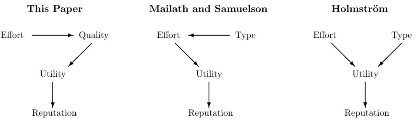
Our paper forms a bridge between classical models of reputation with exogenous types, and models of repeated games. In contrast to the repeated games literature, we suppose there is a state variable which links the periods. In contrast to reputation models, we suppose the state variable is the quality of the firm’s product rather than some exogenous ability type of the firm (see figure 2). As a consequence, long-term dynamics are driven by reputational investment incentives rather than
In their reputation paper, Mailath and Samuelson (2001) consider a firm that sells a good of unknown quality. There are two types of firms: a competent firm who can choose high or low effort, and an inept firm who can only choose low effort. The actual product quality is then a noisy function of the firm’s effort. From the consumer’s perspective, utility is determined by the probability the firm is competent (the firm’s reputation) multiplied by the probability that a competent firm exerts effort.
Mailath and Samuelson derive a striking result: there is a unique Markov perfect equilibrium in pure strategies in which the competent firm always chooses low effort. When the reputation is close to 1, it is impossible to sustain high effort for the same reason as in our paper. Effort then unravels from the top: If the firm is known to be shirking when its reputation passes some cutoff, it has no incentive to exert effort just below this cutoff since success would mean an increase in reputation and an immediate collapse in the price. In contrast, in our paper, product quality is persistent. Thus, the price drifts down continuously when the firm starts to shirk, and unravelling is prevented.
Holmstr¨om (1999) examines a signal-jamming model where an agent of unknown ability can exert effort to confuse the learning of her employer. When the agent’s type is constant, the employer gradually learns the agent’s ability, and effort declines over time. When the agent’s type exogenously changes over time, some effort level is sustained in the stationary equilibrium.
There is a wider literature on reputation models with moral hazard and fixed types, surveyed in Bar-Isaac and Tadelis (2008). A number of these papers examine how a firm’s incentives to exert effort vary over its lifecycle. First, incentives are low towards the end of the firm’s life (Kreps et al. (1982), Diamond (1989)). Second, incentives are low when updating is slow (Benabou and Laroque (1992), Mailath and Samuelson (2001)). Third, when reputation can be lost with one piece of bad news, incentives increase in the level of reputation (Diamond (1989)). Together these papers help explain how demand varies across firms and over time (Foster, Haltiwanger, and Syverson (2008)).3
When compared to the repeated games literature (e.g. Fudenberg, Kreps, and Maskin (1990)), our model has an evolving state variable. Nevertheless, the way that incentives for effort are determined by the signal structure in our paper echoes a similar theme in the repeated games literature. Abreu, Milgrom, and Pearce (1991) and Sannikov and Skrzypacz (2007a) consider a repeated prisoners’ dilemma game with imperfect public monitoring. They find that first-best is attainable as players become patient if the public signal indicates defection (∼bad news), but is not attainable if the public signal indicates cooperation (∼good news) or is generated by Brownian motion.4
3Industry dynamics have been analysed with complete information models with exogenous firm types (Jovanovic (1982), Hopenhayn (1992)) or endogenous capital accumulation (Ericson and Pakes (1995)). The difference between these two approaches is analogous to the distinction between our paper and classical reputation papers.
Skrzy-This Paper Effort Quality Utility Reputation -¡ ¡ ¡ ª ?
Mailath and Samuelson
Effort Type Utility Reputation ¾ @ @ @ R ? Holmstr¨om Effort Type Utility Reputation @ @ @ R ¡ ¡ ¡ ª ?
Figure 2: Relation to Literature. This figure shows the relationships between this paper, Mailath and Samuelson (2001) and Holmstr¨om (1999).
Finally, our paper is related to contract design with persistent effort. Fernandes and Phelan (2000) suppose that an agent’s output depends today on effort both today and yesterday, and derive a recursive formulation to solve for the principal’s optimal contract. Jarque (2008) shows that the problem is much simpler when output depends on the geometric sum of past efforts and the cost of effort is linear. Unlike these papers, our consumers simply react to the firm’s actions, rather than designing contingent contracts.
1.2 Empirical Literature
There are a number of empirical papers examining the importance of reputation in internet auc-tions (eBay). Resnick, Zeckhauser, Swanson, and Lockwood (2006) find that a new seller obtains significantly lower prices than a seller with a good feedback score. Cabral and Horta¸csu (2009) similarly find that a seller with negative feedback obtains significantly lower prices. More interest-ing, Cabral and Horta¸csu (2009) look at the seller’s reactions, showing that a seller who receives one negative feedback is more likely to obtain a second negative feedback, and is more likely to exit. This suggests that either underlying quality is correlated over time, or a seller who receives negative feedback exerts less effort, as in our bad news case.
Studies have also examined the role of reputation in other markets. In the airline industry, a crash reduces the stock market value of the airline and manufacturer in question, reduces demand for all aviation, but increases the value of firms who compete directly with the crashed airline (Chalk (1987), Borenstein and Zimmerman (1988), Bosch, Eckard, and Singal (1998)). In the restaurant market, the introduction of grade cards increased investments in hygiene, and had the biggest effect on non-chain restaurants (Jin and Leslie (2003, 2009)). In the vehicle emission testing market, garages with higher pass rates can demand higher prices (Hubbard (1998, 2002)). In all of these cases, firms make investments that affect the quality of the product, and hence their reputation. While these studies demonstrate the importance in maintaining a reputation, there is pacz (2007b) on simultaneous move games with Brownian and Poisson news.
little evidence on the effect of reputation on the firm’s investment incentives, as examined in this paper.
2
Model
Basics: Timet∈[0,∞) is continuous and infinite. The common interest rate isr ∈(0,∞).
Firm and Consumers: There is one firm and a continuum of consumers. At any point in time
t the firm’s product can have high or low quality, θt ∈ {L = 0, H = µ}, where µ > 0. The
expected instantaneous value of the product to the consumer equals the increment of a stochastic process dZt =dZt(θt, εt) with expected value E[dZt] =θtdt and stochastic component εt that is
independent over time. We will often focus on three functional specifications:
(a) Good news: dZt= 0 almost always but a good product has a breakthrough with arrival rate
µgenerating consumer utility of dZt= 1
(b) Bad news: dZt=µdt almost always but a bad product has a breakdown with arrival rate µ
generating consumer disutility of dZt=−1
(c) Brownian news: dZt=θtdt+dWt
Strategies: At time t the firm chooses effort ηt ∈ [0,1] at cost cηtdt. Product quality θt is
a function of past effort (ηs)0≤s≤t via a Poisson process with arrival rate λ (independent of εt)
that models quality obsolescence. Absent a shock, quality is constant: θt+dt = θt, while at a
shock, previous quality becomes obsolescent and quality is determined by the level of investment:
P r(θt+dt =µ) =ηt. This implies Pr (θt=H) =R0tλeλ(s−t)η
sds+e−λtPr (θ0=H).5
Information: Realized consumer utility dZt is public information, while actual product quality
θtis observed only by the firm.6 The market belief about product qualityx
t= Pr(θt=µ) at time
t is called the firm’s reputation.
Reputation Updating: The reputation increment dxt = xt+dt −xt is governed by realized consumer utility dZt and believed effort ηet. As these are independent, dxt can be decomposed
additively:
dxt=λ(ηet−xt)dt+xt(1−xt)x Pr(dZt|H)−Pr(dZt|L)
tPr(dZt|H) + (1−xt) Pr(dZt|L). (2.1) 5This formulation provides a simple way to allow the firm’s type to depend on its past investments. One can view effort as the choice of absorptive capacity, determining the ability of a firm to recognise new external information and apply it to commercial ends (Cohen and Levinthal (1990)). Equivalently, one could assume the firm first sees the new technology arrive and chooses whether to adopt it at costk=rc/λ.
We denote by dθxt the increments conditional on qualityθ.7
Profit and Consumer Surplus: The firm and consumers are risk-neutral. At time t the firm sets price equal to the expected valueµxt. While consumers get utility 0 in expectation, the firm’s instantaneous profit is (µxt−cηt)dt and its discounted present value is thus given by:
Vθ(x;η,ηe) :=r
Z ∞
t=0
e−rtEθ0=θ,x0=x,η,ηe[µxt−cηt]dt. (2.2)
Markov-Perfect-Equilibrium: We assume Markovian beliefs ηe= ηe(x) and show below that optimal effort η = η(x) is independent of history and current product quality θ. A Markov-Perfect-Equilibrium hη,ηei consists of a Markovian effort function η : [0,1] → [0,1] for the firm and Markovian market beliefs ηe: [0,1]→ [0,1] such that 1) η ∈ η∗(eη) := arg max
η{Vθ(x;η,eη)}
maximizes firm value Vθ(x;η,ηe), given x and ηe, and 2) market beliefs are correct: eη = η. In a Markovian equilibriumη, we will write the firm’s value as a function of its quality and its reputa-tion: Vθ(x).
2.1 Optimal Investment Choice
In principle, the firm’s effort choiceη as well as market beliefsηecould depend on the entire public history dZt = (dZs)0≤s<t, as well as the private history θt = (θs)0≤s<t and time t. We assume
that market beliefs eη are Markovian because we think of the continuum of consumers as sharing their experience in an imperfect way, e.g. through consumer reports. For Markovian beliefs eη, all payoff relevant parameters at timetdepend on the history only via the current product qualityθt
and the firm’s reputationxt. Thus, the optimal effort choice of the firm only needs to depend on
these two parameters.
The benefit of effort in [t;t+dt] is the probability of a technology shock hitting, λdt, times the difference in value functions ∆ (x) :=VH(x)−VL(x), which we call theasset value of quality.
The marginal cost of investment is rc, and thus optimal effortη(x) is given by
η(x) =
(
1 ifrc < λ∆ (x)
0 ifrc > λ∆ (x) . (2.3)
Optimal effort is therefore independent of the current quality of the firmθt. Lemma 1 summarizes this discussion:
7The reason for modelling time as continuous is purely pragmatic. If time were measured in discrete periods, the updating equation (2.1) would be complicated by adt2term because in every period market learning would already take the equilibrium effort decision into account.
Lemma 1 For Markovian beliefs ηe(x) there is an optimal Markovian effort function η(x) that depends solely on the firm’s reputation but not on its product quality. Additionally, η(x) satisfies equation (2.3).
Equation (2.3) makes the model more tractable and is the reason that we assume the cost of effort to be independent of product quality and past effort. An implication of equation (2.3) is that our results are not driven by the asymmetric information about product qualityθ, but solely by the unobserved investment η into future quality. We analyse asymmetric costs in Section??.
2.2 Cutoff Equilibria and Reputational Dynamics
We call an equilibrium work-shirk, if there exists a cutoffx∗ such that a firm with low reputation
x < x∗ exerts effort,η(x) = 1, whereas a firm with a high reputationx > x∗ does not, η(x) = 0. The opposite case, where low reputations shirk and high reputations work, is called a shirk-work
equilibrium.
Reputational dynamics of work-shirk equilibria are fundamentally different from those of shirk-work equilibria. Net of market learning, the dynamicsdx=λ(eηt−xt)dt are convergent in a
work-shirk equilibrium, i.e. dx > 0 for x < x∗ and dx < 0 for x > x∗, but divergent in a shirk-work equilibrium.
A set of reputationsS ⊆[0,1] is called ashirk-hole if the firm shirksη(x) = 0 for allx∈Sand
S is closed under reputational dynamics in that Pr(xt ∈S) = 1 if x0 ∈S. For future use, define
∆x∗(x) to be the asset value of quality for a firm with reputationx when both actual effort ηand
believed effort eη are work-shirk with cutoffx∗.
3
General Results
In this section we prepare the ground-work for the analysis of the good, bad and Brownian news cases. In Section 3.1 we derive the welfare maximising effort. As noted above, the firm’s value
Vθ(x) is a function of it’s reputation and quality. In Section 3.2 we show that an increase in reputation increases the price today and tomorrow, and therefore increases Vθ(x). In Section 3.3 we show that a higher quality derives its value indirectly, through its effect on future reputation. In particular, Theorem 1 interprets the asset value of quality as the net present value of future reputational dividends. Finally, Section 3.4 derives some general results about the firm’s effort choice.
3.1 Welfare
Suppose product quality is publicly observed. Then the benefit of exerting effort equals the obso-lescence rateλtimes the price differentialµdivided by the effective discount rater+λ. Thus the
first-best effort choice is given by: η= ( 1 ifc < λ r+λµ 0 ifc > r+λλµ . (3.1)
There is no equilibrium with positive effort if c > r+λλµ. In this case, welfare is negative and the firm makes negative profits as consumers receive zero utility in equilibrium. The firm therefore prefers to shirk at all levels of reputation, thereby guaranteeing itself a non-negative payoff.
We thus restrict attention in the paper to the casec < r+λλµ. 3.2 Value of Reputation
Lemma 2 shows that, when the firm is choosing its effort optimally, the value function is increasing in reputation.8 To prove the lemma, we need to rule out the possibility that a firm with a higher
initial reputation may shirk, lose its product quality, and fall behind a firm with a lower initial reputation. We do this by observing that a firm always has the option to mimic a firm with a slightly lower reputation.
Lemma 2 Given an optimal response to market beliefs η∗(ηe), the value function of the firm
Vθ(x;η∗(ηe),ηe) is strictly increasing in its reputation x and increasing in market beliefsηe.
Proof. Fix θ, (x0,eη0) and (x00,eη00) ≥ (x0,ηe0), i.e. x00 ≥ x0 and ηe00(x) ≥ ηe0(x) for all x. Write the best response η∗(ηe0) to the Markovian beliefs ηe0 in a non-Markovian way as a function of the public historyη(dZt) =η¡x¡dZt,ηe0, x0¢¢. For any realization of the random processes, denote by (x00
t, θ00t, ηt00, dZt00) the trajectory of reputation, quality, effort and utility given effort η(dZt), initial
reputation x00 and market beliefs eη00, and by (x0
t, θ0t, η0t, dZt0) the corresponding trajectory given
η, x0,ηe0.
By construction, effortη0
t=ηt00, qualityθt0 =θt00, and utilitydZt0 =dZt00will coincide for all times
t. Reputation on the other hand may start at different levels x00 ≥ x0 and because the updating equation (2.1) implies that xt+dt(xt,ηet, dZt) is increasing in xt and eηt, we getx00t ≥x0t.
Thus, by mimicking the effort of the firm with lower initial reputation x0, the firm with a strictly higher initial reputation x00 can secure itself a strictly higher value. By Lemma 1 there must be a Markov strategy that is at least as good as this mimicking strategy. ¤
Lemma 2 implies that across equilibria η, η0, with η0(x) ≥ η(x) for all x, the firm’s value is increasing in effort Vθ(x;η0, η0)≥Vθ(x;η, η).
8While it is unclear whether these monotonicity results hold for non-equilibrium hη,eηi, Lemma 6 in Appendix C.1 extends them to work-shirk effort functions where the cutoff typex∗is indifferent between working and shirking.
3.3 Value of Quality
As shown in Section 2.1, investment incentives are driven by the asset value of quality ∆ (x). To analyse this value, we can decompose it into (a) the immediate benefit of a positive market signal, called the reputational dividend, and (b) the continuation benefit of a high quality product:
∆(x) = (1−rdt)(1−λdt)Ex[VH(x+dHx)−VL(x+dLx)] (3.2)
= (1−rdt−λdt)Ex[(VH(x+dHx)−VH(x+dLx)) + ∆(x+dLx)].
The first line uses the principle of dynamic programming, while the second adds and subtracts
VH(x+dLx). Integrating up yields equation (3.3) in Theorem 1, which expresses the asset value
of quality as the discounted sum of future reputational dividends. Equation (3.4) follows from the alternative decomposition of (3.2) when we add and subtractVL(x+dHx) instead ofVH(x+dLx). These expressions serve as a work-horses throughout the paper.
Theorem 1 Fix any Markovian beliefsηeand a Markovian best responseη∗(ηe). Then two closed-form expressions for the value of quality ∆ (x) are given by
∆(x) = Z ∞ 0 e−(r+λ)tEx0=x,θt=L[DH(xt)]dt (3.3) = Z ∞ 0 e−(r+λ)tEx0=x,θt=H[DL(x)]dt (3.4) where θt=L is short for θs =L for all s∈[0;t], and the reputational dividend Dθ(x) is defined by
Dθ(x) :=E[Vθ(x+dHx)−Vθ(x+dLx)]/dt.
Proof. To integrate up (3.2), fix xand setψ(t) :=Ex0=x,θt=L[∆(xt)]. Up to terms of order o(dt)
we have −d ³ ψ(t)e−(r+λ)t ´ = −e−(r+λ)t(ψ(t+dt)−ψ(t)−(r+λ)dtψ(t)) = e−(r+λ)tEx0=x,θt=L[−Ext[∆(xt+dLxt)] + (1 + (r+λ)dt) ∆(xt)] = e−(r+λ)tEx0=x,θt=L[DH(xt)]dt and (3.3) follows. ¤
Corollary 1 Fix any Markovian beliefs ηe and a Markovian best response η∗(ηe). For a given reputation x, a high-quality firm has a higher value than a low-quality firm, i.e. VH(x)≥VL(x).
Proof. By the updating equation (2.1) we have dHx ≥ dLx, by Lemma 2 we get Dθ(x) =
3.4 Investment Levels
Lemma 3 (Some Effort Somewhere) For sufficiently low costs c, pure shirking, i.e. η(x) = 0
for all x, is not an equilibrium.
Proof. Fixing η(x) = ηe(x) = 0, value functions and ∆ do not depend on c, and ∆ (x) > 0 for somex. Thus, as the cost of effort vanishc→0, its benefitsλ∆ (x) are constant and thus bounded away from 0, contradicting the equilibrium condition. ¤
This result is in contrast to reputational models with inept firms where shirking is always an equilibrium, even if costs of working are 0. As discussed in the introduction the critical difference in this model is that expected quality and price still depend on the firm’s reputation - and in particular are greater than 0 - even when the firm is believed to be shirking.
Lemma 4 (No Effort at the Top) If no market signal dZt perfectly reveals low quality, i.e. if Pr(dZt|L)
Pr(dZt|H) <∞ for alldZt, then a firm with a perfect reputationx= 1must be shirking with positive probability: η(1)<1.
Proof. Assume to the contrary thatη(1) = 1 in equilibrium. By the assumption that Pr(Pr(dZtdZt||HL)) <
∞, a firm with perfect reputationx= 1 can never lose its reputation, irrespectively of the consumer utilitydZtit generates. Thus dHxt=dLxt= 0 and by Theorem 1 the asset value of quality ∆ (x) equals 0. Thus, η(1) = 1 cannot be sustained in equilibrium. ¤
The proof actually shows a slightly stronger statement: In no equilibrium the firm can be working for all reputation levels xin an interval of arbitrary high reputations (1−ε,1).
4
Good News
Assume that consumers learn about qualityθt from infrequent product breakthroughs that reveal
θ =H with arrival rate µ. Absent a breakthrough, updating evolves deterministically according to:
dx
dt =λ(η(x)−x)−µx(1−x). (4.1)
We define xt as the deterministic solution of the ODE (4.1) with initial valuex0.
The reputational dividend, which is the value of having a high quality in the next instant, equals the value of increasing the reputation fromx to 1 times the probability of a breakthrough:
Conditioning on the firm always being low quality, in order to prevent a breakthrough, the time path of reputation is given by (4.1). Using equation (3.3), the asset value of quality is:
∆(x0) =
Z ∞
0
e−(r+λ)tµ[VH(1)−VH(xt)]dt (4.2) The reputational dividend VH(1)−VH(xt) is decreasing inxt, so that ∆(x0) is decreasing in x0.
It follows that any equilibrium is work-shirk. Intuitively, when a breakthrough occurs the firm’s reputation immediately jumps to 1. Since this jump is larger for a low-reputation firm, incentives to invest decrease in reputation and the equilibrium is work-shirk.
The form of the equilibrium implies that the reputational dynamics converge to a cycle. Absent a breakthrough, the firm’s reputation converges to a stationary point ˆx= min{λ/µ, x∗}where the firm works with positive probability. When a breakthrough occurs, the firm’s reputation jumps to 1. The firm is then believed to be shirking, so its reputation drifts down to ˆx, absent another breakthrough. In the long-run, the firm’s reputation therefore cycles over the range [ˆx,1].
Theorem 2 In the good news case (a) Every equilibrium is work-shirk.
(b) Reputational dynamics converge to a non-trivial cycle. (c) If λ≥µ, the equilibrium is unique.
(d) For sufficiently high λ, zero-effort is the only equilibrium.
Proof. Part (a). Reputation xt follows (4.1), so an increase in x0 raises xt at each point in
time. Lemma 2 says thatVH(x) is strictly increasing inx, so equation (4.2) implies that ∆(x0) is
decreasing in x0. Part (b) follows from (a).
Part (c). We will show that ∆x∗(x∗) is decreasing in x∗. Under the assumption λ ≥ µ,
the reputational dynamics xt starting at cutoff x0 = x∗ are stuck at x∗. Thus, by equation
(4.2) the value of quality is the discounted present value of an reputational boost from x∗ to 1: ∆x∗(x∗) = µ
r+λ(VH,x∗(1)−VH,x∗(x∗)). In Appendix A.1 we show that the latter term is given by
VH,x∗(1)−VH,x∗(x∗) = Z ∞ t=0 e−rtrµ(xt−x∗) · λ λ+µ+ µ λ+µe −(µ+λ)t ¸ dt, (4.3) where x0 = 1. Note that, in this expression, the terms in the brackets capture the possibilities of
λand µshocks while xt descends from 1 to x∗. Equation (4.3) is decreasing in the cutoff, so the
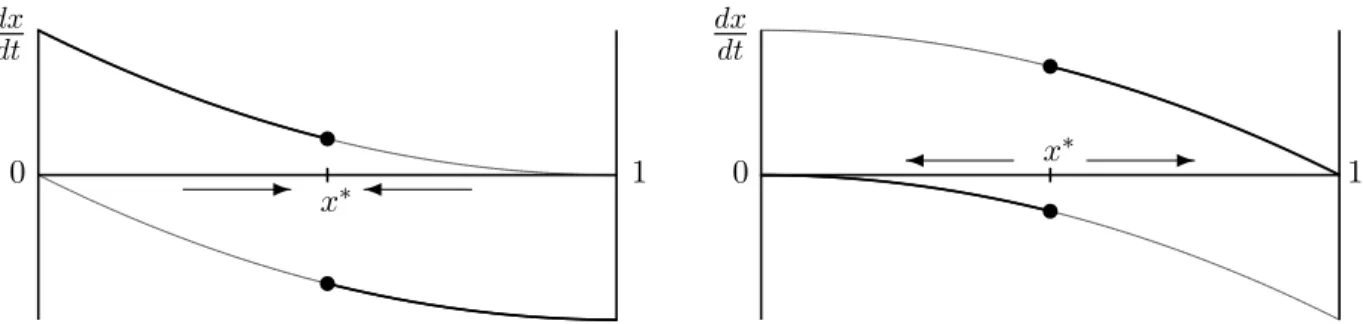
t t t t - ¾ ¾ -dx dt dxdt 0 1 0 1 x∗ x∗
Figure 3: Dynamics in Good News (left) and Bad News (right). This picture illustrates how the reputational driftdx/dt, absent a breakthrough, changes with the reputation of the firm,x. These pictures assumeλ=µand x∗= 1/2. The dark line shows the drift when beliefs are correct.
Part (d). Letx∗ = 0. Using part (a) andxt≤e−λt, we get
λ∆0(0)≤ r+λλµ Z ∞ t=0 e−(r+λ)trµ dt= λ r+λ rµ2 r+λ
When λis sufficiently high λ∆0(0)< rc, and the unique equilibrium exhibits zero effort. ¤
Suppose thatλ≥µ, so the firm’s reputation drifts up whenever it is known to be working (see figure 3). In this case, the dynamics are stationary at ˆx=x∗, at which point the firm chooses to work with probabilityη(x∗) =x∗¡1 +µ
λ(1−x∗)
¢
so as to keep its reputation constant.
Theorem 2(c) shows that the equilibrium is unique. To understand this result, suppose the market believes the cutoff is ˜x, and denote the firm’s best response by x∗(˜x). An increase in ˜x
means the firm’s reputation will not drift down as far, absent a breakthrough. This change benefits low-quality firms more than high-quality firms, reducing ∆(x). As a result, x∗(˜x) is decreasing in ˜
x and there is a unique fixed point where x∗(˜x) = ˜x.
Theorem 2(d) says that, as technology shocks become more frequent the incentives to exert effort disappear. Intuitively, when λis high, equilibrium beliefs move the reputation towards x∗ very quickly. Hence a breakthrough, which raises the reputation to 1, is quickly depreciated. This means there is little value to being a high-quality firm and little value to investing. Theorem 2(d) implies that investment is non-monotonic in the frequency of technology shocks. When shocks are too frequent, equilibrium beliefs drive reputation and there is no incentive to invest in actual quality. When shocks are too infrequent, investment takes too long to pay off and, again, there is little incentive to invest in quality. For intermediate frequencies, however, effort can be supported.
5
Bad News
Assume that xt is generated by breakdowns that reveal θ = L with arrival rate µ. Absent a breakdown, updating evolves deterministically according to:
dx
dt =λ(η(x)−x) +µx(1−x). (5.1)
We define xt as the solution of the ODE (5.1) with initial value x0.
The reputational dividend, which is the value of having a high quality in the next instant, equals the value of not losing one’s reputation times the probability of a breakdown:
DL(x) =VL(xt+dHxt)−VL(xt+dLxt) =µ(VL(xt)−VL(0))dt.
Conditioning on the firm always being high quality, in order to prevent a breakdown, the time path of reputation is given by (5.1). Using equation (3.4), the asset value of quality is:
∆(x0) =
Z ∞
0
e−(r+λ)tµ[VL(xt)−VL(0)]dt. (5.2)
The jump size VL(xt)−VL(0) is increasing in xt, so that ∆(x) is increasing in x. It follows that
any equilibrium is shirk-work. Intuitively, when a breakdown occurs a firm immediately jumps to reputationx= 0. Since this jump is larger for a high-reputation firm, incentives to invest increase in reputation and the equilibrium is shirk-work.9
The form of the equilibrium implies that the reputational dynamics diverge. Suppose we are in an equilibrium withx∗∈(0,1), so firms belowx∗ shirk while firms abovex∗ work. A firm that starts with reputation above x∗ converges to reputation x = 1, absent a breakdown. If the firm is hit by such a breakdown while its product quality is still low, it gets stuck in a shirk-hole with reputation x= 0. A firm with reputation below x∗ initially shirks and may have either rising or falling reputation, depending on parameters. In either case, its reputation will either end up at
x= 0 orx= 1.
To allow for positive effort in some equilibrium we impose the following assumption:
λ
r+λ+µµ(µ−c)> rc (PE)
Theorem 3 Assume (PE) holds. In the bad news case
9For example, when writing about the explosion of Sony’s batteries in Dell’s laptops the Financial Times wrote that “The withdrawal comes at a sensitive time for [Dell], which has been fighting broader perceptions of poor customer service and slowing sales growth. [However] it could have a deeper impact on Sony, given the Japanese company’s reputation for quality in the consumer electronics industry”(15th August 2006). This illustrates the point that the jump in reputation is larger for higher reputation firms.
(a) Every equilibrium is shirk-work.
(b) If x∗∈(0,1)then reputational dynamics diverge to 0 or 1.
(c) If λ ≥ µ there is a non-empty interval [a, b] such that every cutoff x∗ ∈ [a, b] defines an equilibrium.
(d) If λ is sufficiently high, everyx∗∈(0,1]defines an equilibrium.
Proof. Part (a). Reputation xt follows (5.1), so an increase in x0 raises xt at each point in
time. Lemma 2 says thatVL(x) is strictly increasing inx, so equation (5.2) implies that ∆(x0) is
increasing in x0. Part (b) follows from (a).
Part (c). If λ ≥ µ, the dynamics are divergent at x∗: if x
0 = xt−², then limxt = 0; if
x0 = xt+², then limxt = 1. Thus, to define value functions and ∆ at the cutoff x∗ we need to
specify whether or notx∗ works. Denote by ∆−
x∗(x) (resp. ∆+x∗(x)) the value of quality atx when
x∗ is believed to be shirking (resp. working). At x∗ ∈(0,1) we have ∆−
x∗(x∗) = limx%x∗λ∆x∗(x)
and ∆+x∗(x∗) = limx&x∗λ∆x∗(x). Lemma 2 says that VL(xt) is strictly increasing in xt, so (5.2)
implies that
∆−x∗(x∗)<∆+x∗(x∗). (5.3)
A cutoff x∗ ∈(0,1] then defines a shirk-work equilibrium iff10
λ∆−x∗(x∗)≤rc≤λ∆+x∗(x∗). (5.4)
Equation (5.2) implies that ∆+x∗(x∗) and ∆x−∗(x∗) are increasing and continuous inx∗. For the lower
bound, observe thatλ∆−0(0) = 0, because a firm with no reputation that is believed to be shirking is stuck at 0 forever. For the upper bound,λ∆+1(1) = r+λλ+µµ(µ−c) becauseVL,1(1) = r+r+λ+λµ(µ−c),
VL,1(0) = 0, and λ∆+1(1) = rλµ+λ(VL,1(1)−VL,1(0)). Under assumption (PE) equation (5.4) therefore defines a non-empty interval of cutoffs, [a, b].
Part (d). Pick anyx∗ >0. First, supposex
0 > x∗and observe thatxt≥1−e−λt. In Appendix
B.1 we derive the following formula for the value of quality: ∆x∗(x) = µ
λ+µ
Z ∞
t=0
e−rtr(µxt−c)(1−e−(λ+µ)t)dt (5.5) 10The casex∗= 0 is more subtle because there are two qualitatively different effort-profiles with cutoffx∗= 0.
Ifx∗= 0 is believed to be working, there is no shirk-hole, and the necessary and sufficient condition for equilibrium
is that this is in the firm’s best interest, i.e. rc≤λ∆+ 0(0).
However, if x∗ = 0 is believed to be shirking, then x∗ = 0 is a shirk-hole and the equilibrium condition is
rc≤λ∆−
0 (x) for allx >0 (andrc≥λ∆−0 (0) which is automatically satisfied becauseλ∆−0 (0) = 0). This condition is weaker than (5.4) as ∆+
0 (0)<limx→0∆−0 (x): The existence of a shirk-hole increases the value of quality. Formally, this is reflected in equation (5.2) in thatVL(0) = 0 if reputation 0 shirks, butVL(0)>0 if reputation 0 works.
Taking limits, lim λ→∞λ∆x ∗(x)≥ lim λ→∞ λµ λ+µr Z ∞ t=0 e−rt(µ(1−e−λt)−c)(1−e−(λ+µ)t)dt=µ(µ−c)
where the final equality uses the fact that the integral converges to (µ−c)/r. Assumption (PE) implies that µ(µ−c) > rc. Hence for sufficiently large λ, working is optimal for all x > x∗ and any x∗.
Next supposex0 < x∗and observe thatxt≤e−(λ−µ)t. In Appendix B.1, we derive the following
formula for the value of quality:
∆x∗(x) = µ λ−µ Z ∞ t=0 e−rtrµxt(e−µt−e−λt)dt (5.6) Taking limits, lim λ→∞λ∆x∗(x)≤λlim→∞ λµ λ−µ Z ∞ t=0 e−rtrµe−(λ−µ)tdt= 0 Hence for sufficiently large λ, shirking is optimal for all x < x∗ and any x∗. ¤
Supposeλ≥µ, so that whenever the firm is known to be shirking its reputation drifts down (see figure 3). In this case, the region below x∗ is a shirk-hole: when a firm’s reputation is below the cutoff, it is certain to see its reputation decrease because of the unfavourable equilibrium beliefs. Such a firm always shirks, eventually giving rise to a low quality product and a product breakdown destroying whatever is left of its reputation. When a firm’s reputation is above the cutoff, favourable market beliefs contribute to an increasing reputation and the firm invests to insure itself against a product breakdown. At the cutoff, the firm works when it is believed to be working and shirks whenever it is believed to be shirking.11
Theorem 3(c) shows that there is an interval of equilibrium cutoffs satisfying (5.4). The multi-plicity is driven by a discontinuity in the value function atx∗, caused by the divergent reputational dynamics. Intuitively, the market’s beliefs become self-fulfilling. If the market believes the firm is shirking, it’s reputation falls, undermining any incentive to invest. Conversely, if the market believes the firm is working, its reputation rises, causing the firm to invest in order to protect its appreciating reputation.
When λ < µ the dynamics have additional interesting features: Define bx = 1− λµ ∈ (0,1) to be the stationary point in the dynamics when the firm is believed to be shirking. There are two types of equilibria:
1. Trapped equilibria. When x < xb ∗, a firm with reputation x ∈ (0, x∗) finds its reputation converging to bx, and remains stuck in a shirk-hole. At some point is suffers a breakdown
11The divergent dynamics imply that there will be path dependence in reputations. This is consistent with the existence of credit traps in financial markets, and may help explain why political scandals have such dramatic effects on politicians careers (Diermeier, Keane, and Merlo (2005)).
and remains at x= 0 thereafter. Since the dynamics are divergent atx∗ the value function is discontinuous, and there is an interval of such equilibria.
2. Permeable equilibria. When x > xb ∗, a firm with reputation x∈(0, x∗) finds it’s reputation increasing. Ifxtpassesx∗before a breakdown hits, the firm starts to work and it’s reputation
may converge to one. Since the value functions are continuous at a permeable cutoffx∗, there is at most one permeable equilibrium.
Finally, Theorem 3(d) shows that as technology shocks become more frequent, then any cutoff can be an equilibrium. Intuitively, a firm that starts below the cutoff finds it’s reputation falling to zero instantly and gives up, while a firm above the cutoff finds it’s reputation rising to one instantly and works to stay there. While outside the model, this multiplicity creates an incentive for firms to invest in marketing in order to shape consumers expectations.
6
Brownian News
We now assume that consumers learn about quality θt gradually, through the evolution of a
Brownian motion with state-dependent drift,dZt=θtdt+dWt. Updating evolves according to
dHx = λ(η(x)−x)dt+µ2x(1−x)2dt+µx(1−x)dW (6.1)
dLx = λ(η(x)−x)dt−µ2x2(1−x)dt+µx(1−x)dW.
To calculate the value of quality we apply Itˆo’s formula to get: Ex[Vθ(x+dHx)] = Vθ(x) +µ2x(1−x)2Vθ0(x)dt+ (µx(1−x))2 2 V 00 θ (x)dt Ex[Vθ(x+dLx)] = Vθ(x)−µ2x(1−x)2Vθ0(x)dt+ (µx(1−x))2 2 V 00 θ (x)dt.
The reputational dividend is thus:
DH(x) =Ex[VH(x+dHx)−VH(x+dLx)]/dt=µ2x(1−x)VH0 (x). (6.2)
DH(x) declines to zero in either tail as reputational updating becomes very slow. Using equation
(3.3), the value of quality reduces to ∆(x) =
Z ∞
0
e−(r+λ)tEx0=x,θt=L[µ2xt(1−xt)VH0 (xt)]dt. (6.3)
Theorem 4 shows that, for small costs, there exists an equilibrium whereby the firm works when its reputation is below some cutoff, x∗. In such an equilibrium, the reputation of a firm below
the cutoff tends to rise, whereas the reputation of a firm above the cutoff tends to fall, leading to cyclical dynamics. Theorem 4 also shows that, for small costs, this equilibrium is essentially unique in that (i) the work-shirk cutoff is unique; and (ii) the work region in the work-shirk equilibrium is arbitrarily close to the work-region in any other equilibrium. Denote the work region in an arbitrary equilibrium by Rη = {x : η(x) = 1} and let R∗ be the work-region in the work-shirk
equilibrium. Let h be the Hausdorff metric.
Theorem 4 There isc∗ such that for all c∈(0, c∗):
(a) There exists x∗ ∈(0,1) such that work-shirk with cutoff x∗ is an equilibrium. (b) Reputational dynamics converge to a non-trivial cycle.
(c) Equilibrium is essentially unique: (i) The work-shirk cutoff x∗ is uniquely determined; and (ii) h(Rη, R∗)< ², for any equilibrium η and any ² >0.
(d) For fixed c and high enough λ, there is no work-shirk equilibrium, but zero-effort is an equilibrium.
Proof. See Appendix C. ¤
Section 6.1 discusses the existence of work-shirk equilibria. Section 6.2 considers other forms of equilibria. Section 6.3 discusses the effect of a high obsolescence rate (λ→ ∞).
6.1 Work-Shirk Equilibria
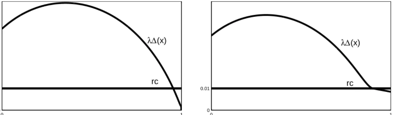
When costs are low, there is a work-shirk equilibrium but no shirk-work equilibrium (Lemma 4). This asymmetry is illustrated in the left panel of figure 4. Intuitively, when the firm is believed to be working, the asset value of quality is zero atx= 1 since current dividends are zero and, as the firm’s reputation stays at x= 1, future dividends are zero. In contrast, the asset value of quality is positive atx= 0 since the market’s belief that the firm is working causes its reputation to drift into the interior of (0,1), enabling it to collect high dividends in the future. In other words, the firm wishes to invest at x = 0 not because immediate reputational dividends, which are close to 0, but because of future dividends, when the firm’s reputation is sensitive to true quality.
Figure 4 is almost a proof of Theorem 4(a). Elementary calculations show that: ∆1(x) ( >0 forx <1 = 0 for x= 1 and ∆ 0 1(1)<0.
0 1 0 0.01 Reputation, x λ∆(x) rc 0 1 0 0.01 Reputation, x λ∆(x) rc
Figure 4: Asset Value of Quality under Full Effort (left) and in Work-Shirk Equilibrium (right). This figure assumes that µ= 1, λ= 1, r = 1 and c = 0.01. In the work-shirk equilibrium, the resulting cutoff is isx∗= 0.900.
and thus for small cthere existsx∗ such that
λ∆1(x)
> rc forx < x∗ (Low reputations work) =rc forx=x∗ (x∗ indifferent)
< rc forx > x∗ (High reputations shirk).
(6.4)
To prove part (a) we just need to replace ∆1 on the LHS with ∆x∗. The problem with this simple
argument is that it implicitly assumes continuity of ∆0
x∗ asx∗ →1. However, it is straightforward
to show that limx∗→1∆0x∗(1) = 0>∆01(1). As a result, it could be that ∆x∗(x) is increasing inx
forx > x∗, contradicting the last condition in (6.4).
To understand this complication, consider the marginal value of reputation V0
θ(x) to a firm
with reputation x∈[x∗,1] wherex∗ ≈1. A reputational incrementdxis valuable to the firm only as long asxt|x0=x+dx> x∗: As soon asxt|x0=x+dx=x∗ the incrementxt|x0=x+dx−xt|x0=xvanishes
because of the difference of driftE[dx] to the left ofx∗ and to the right ofx∗. As a consequence,
V0
θ(x) and Dθ(x) may be minimized at the cutoff x∗, and one may be concerned that ∆x∗(x) is
also minimised atx∗.
To overcome this complication and show that λ∆x∗(x∗) > λ∆x∗(x) for x ∈ (x∗,1] we need
a better understanding of the reputational dynamics dx and the marginal values V0
θ,x∗(x) for
x, x∗ ≈1. Fortunately, the dynamics of (1−x) approximate a geometric Brownian motion which is reflected at (1−x∗) by the large relative difference in the drift terms. For the high quality firm,
dH(1−x) = −λ(η−x)dt−µ2x(1−x)2dt+µx(1−x)dW ≈
(
−λ(1−x)dt−µ(1−x)dW forx < x∗
0 1 0 0.06 Value of Quality Reputation, x rc λ∆(x)
Figure 5: Shirk-Work-Shirk Equilibrium. This figure illustrates the asset value of quality in a work-shirk equilibrium, ∆x∗(x). The straight line equalsrc/λ. This figure assumes thatµ= 1,λ= 1,r= 1 and
c= 0.06. The resulting cutoffs arex= 0.910 and x= 0.958.
and likewise fordL(1−x).
This has two implications. First, while the dividend may be minimised at x∗, the value of quality at the cutoff ∆x∗(x∗) is largely determined by the dividends at x < x∗. Second, the
marginal value of reputation and the dividend atx > x∗ are small in relation to those atx < x∗. This is because a reputational increment essentially disappears when xt = x∗ and this happens much sooner for initial reputations x0 > x∗ than for x0 < x∗. Hence for x > x∗, ∆x∗(x) is an
average of low dividends while xt > x∗, and a continuation value ∆x∗(x∗) when xt hits x∗. This
average comes to less than ∆x∗(x∗), as required.
6.2 Other Equilibria
Given that reputational updating is slow at x≈0 andx≈1, one may expect there to exist shirk-work-shirk equilibria, where a firm works when its reputation is between two cutoffs,x∈[x, x] and shirks elsewhere. A firm with a low reputation is thus trapped in a lower shirk-hole in which market learning is too slow to incentivise effort, while a firm above x experiences convergent dynamics around x.
Simulations indicate that such equilibria may exist for certain parameter ranges (figure 5). Investment incentives in this equilibrium (withc= 0.06) are much higher than in the above work-shirk equilibrium (withc= 0.01). This is because a firm at the work-shirk cutoff has more to lose when a sequence of bad utility draws can push its reputation into a shirk-region, where it may be stuck forever.
For low costs, Theorem 4(c) shows that shirk-work-shirk equilibria disappear because a firm at the shirk-work cutoff x strictly prefers to work. Intuitively, reputational dividends and the value of quality are uniformly bounded below on any interval [ε; 1−ε] so, when costs are small,
all intermediate reputations prefer to work. At the lower cutoff,x, working is then very profitable since it can make the difference between falling into the shirk-hole and sinking to x = 0, and climbing into the work region and rising tox=x.
While no shirk-work-shirk equilibria exist for low costs, there may be other equilibria. However, these extra equilibria are qualitatively similar to the work-shirk equilibrium and can be charac-terised by {x, x} with η(x) = 1 for x < x and η(x) = 0 for x > x.12 These equilibria all involve
work on [0,1−²], so they converge to the work-shirk equilibrium in the Hausdorff metric asc→0. Moreover, the work-shirk transitions act like reflection barriers implying that x ≈ x∗, so these extra equilibria entail as least as much work as the work-shirk equilibrium.
6.3 High Obsolescence Rate
Theorem 4(d) states that, for sufficiently highλ, the work-shirk equilibria disappear and zero-effort is an equilibrium. The intuition is the same as in the good news case: The high drift towards a work-shirk cutoff x∗ ∈(0,1) drives the marginal value of reputation to 0, and with it the reputational dividend and the value of quality. Zero-effort is an equilibrium because the drift towards 0 ensures low values of xt, and with this a diminishing reputational dividendDθ(x) =µ2x(1−x)Vθ0(x).
We conjecture that zero-effort is the unique equilibrium as λ → ∞, as suggested by our numerical simulations. For example, with a shirk-work-shirk profile, the need to incentivise effort atx=ximplies that the size of this region, x−x, must become small so that having high-quality affects the probability of falling into the shirk region. However, asx−xbecomes sufficiently small, the probability of entering the shirk region grows, andV (x) and ∆ (x) converge to 0.
7
Extensions
7.1 Generalized Poisson-Learning
We focused above on good, bad and Brownian news for the sake of clean analytical results. We now discuss how the qualitative insights can shed light on market learning via more general Poisson processes.
7.1.1 Good and Bad News
Assume that the product can enjoy both breakthroughs revealing high quality with intensityµH, and breakdowns revealing low quality with intensityµL. In this case the reputational dividend is 12For example, given the parameters in figure 4, there is another equilibrium with working on [0,0.900], shirking on [0.900,0.944], working on [0.944,0.9605] and shirking on [0.9605,1].
given by:
Dθ(x) = µH(Vθ(1)−Vθ(x)) +µL(Vθ(x)−Vθ(0))
= (µL−µH)Vθ(x) +µHVθ(1)−µLVθ(0).
Assume further that breakdowns are more likely than breakthroughs: µL > µH. This case is
similar to the pure bad news case of section 5:13 Reputational dividend and value of quality are
increasing in reputation, and any equilibrium must be shirk-work.
However, parts (b), (c) and (d) of Theorem 3 no longer hold true: Equilibrium dynamics are similar, but now a shirking low-reputation firm with a high product quality may escape the shirk-hole with a product breakthrough. This renders the value of quality atx= 0 strictly positive, even under adverse market beliefs. Thus, proper shirk-work equilibria, where x= 0 shirks and x = 1 works, fail to exist for low c. While incentives can thus be too high for any proper shirk-work equilibrium, they can at the same time be too low for a full-work equilibrium, e.g. for high values of λ, and equilibrium may fail to exist.14
7.1.2 Generalized Bad News
We now modify the bad news case by allowing for occasional failures of high-quality products with intensity µH < µL, as is common in the literature, e.g. Abreu, Milgrom, and Pearce (1991).
While a product breakdown still causes a discrete hit to the firm’s reputation it does not destroy it completely. Lemma 4 states that in equilibrium a firm with a perfect reputation cannot believed to be working. However, the insights of the bad news section are robust to this variation in that, for low costs c, we can still show the existence of shirk-work-shirk, and work-shirk equilibria (rather than work-shirk and full work equilibria in the case of pure bad news).15
The shirk-work-shirk equilibrium captures the idea that a product breakdown can put a firm in the “hot-seat” where one more breakdown would finish the firm off, by pushing it into a shirk-hole.
13The alternative case, withµH> µL, is similar to the pure good news case of section 4. Finally, when quality is discovered with equal intensity,µH=µL, incentives are flat and either full-effort or zero-effort is an equilibrium.
14This argument does not yet prove that for certain parameter ranges equuilibrium does not exist: For even if incentives are too high for a proper shirk-work equilibrium (and too low for a full-effort equilibrium), they need not be too high for a zero-effort equilibrium.
15To prove this we need to slightly adopt the equilibrium existence proof for Brownian learning in Appendix C: For the work-shirk equilibrium, the only remarkable difference is that an extra term appears in equation (C.4) as the discontinuous reputation dynamics may now jump over the cutoff. However, this term can be matched by an equivalent term - for the firm with initial reputation`∗when it suffers a breakdown - which outweighs the first term
by Lemma 9.
The shirk-work-shirk equilibrium on the other hand is in contrast to the Brownian case, in particular to Lemma 12. The key difference is that value functions are now discontinuous, incentivising effort above the cutoff but not in the shirk-hole just below. To construct the shirk-work-shirk equilibrium, we can first choose the lower, shirk-work cutoff low enough so as to discourage work in the shirk-hole, and then reapply the arguments in Appendix C to prove existence of the upper, work-shirk cutoff with the required properties.