Weakly-Supervised Temporal Activity Localization and Classification With Web Videos

(1)

UC Riverside

UC Riverside Electronic Theses and Dissertations

Title

Permalink

https://escholarship.org/uc/item/6sw159w4

Author

Dougherty, Thomas

Publication Date

2019 Peer reviewed|Thesis/dissertation

(2)

UNIVERSITY OF CALIFORNIA RIVERSIDE

Weakly-Supervised Temporal Activity Localization and Classification With Web Videos

A Thesis submitted in partial satisfaction of the requirements for the degree of

Master of Science in Electrical Engineering by Thomas Dougherty September 2019 Thesis Committee:

Dr. Amit K Roy-Chowdhury, Chairperson Dr. Salman Asif

(3)

Copyright by Thomas Dougherty

(4)

The Thesis of Thomas Dougherty is approved:

Committee Chairperson

(5)

Acknowledgments

I am grateful to my advisor, Dr. Amit Roy-Chowdhury, for welcoming me into his lab. I’d like to thank him for acknowledging my curiosity in this field and allowing me to pursue this research direction. His passion and drive for this field has been nothing but inspiring for me, and has allowed me to internalize that anything I do in life must be done with both tenacity and love. I am grateful to have him as an advisor, where his expertise and wisdom has helped guide and complete my journey here at UCR. I’d like to thank Sujoy Paul for allowing me to build upon his research. I especially would like to thank him for the guidance and help he has provided me. Sujoy’s expertise and time spent on me was invaluable and without him, this thesis would not be possible. I am grateful of everything that he has provided. Although not needed, I wish him the best of luck and fortune to all his future endeavors.

I am grateful for my girlfriend Pamela, for taking a trip with me along this expe-rience. I thank her for being there with me when I needed it the most. I also thank her for the financial support she provided me throughout my time in graduate school. I’d like to thank my friends Evan and Justin for being nothing but support and friendship throughout my time at UCR. I love you both.

I would like to thank my Mom, Hee Dougherty, for pushing me to go to college. She sacrificed her life to give me the opportunities and future I currently hold. This is a debt I will forever hold. I will always appreciate and love you. I would like to thank my Dad, Dennis Dougherty. This Master’s is dedicated to you.

(6)

(7)

ABSTRACT OF THE THESIS

Weakly-Supervised Temporal Activity Localization and Classification With Web Videos by

Thomas Dougherty

Master of Science, Graduate Program in Electrical Engineering University of California, Riverside, September 2019

Dr. Amit K Roy-Chowdhury, Chairperson

In this thesis, weakly-supervised temporal activity localization and classification is considered with the use of web videos. Most activity localization methods depend on the availability of frame-wise annotation, which is a burdensome task to collect. To reduce the effort of manual labeling, learning from weak labels may be used as a potential solution. Recently there has been a substantial influx of tagged videos on the Internet. These can potentially be used as a rich source of data for weakly-supervised training. The following problem is considered. Given only the keyword of an action, can videos be retrieved online and be used to train the Weakly-Supervised Temporal Activity Localization and Classifi-cation (W-TALC) network? Then, can a re-ranking method be implemented to filter out noisy video data? Action categories of the Thumos14 dataset are used to search for videos online with Youtube Data API. These videos are used as a training set for the W-TALC network. Given only the video labels, the W-TALC network learns to both localize and classify actions in videos. Using a re-ranking strategy, noisy video data is removed and shows an increase in detection performance versus using the original web video dataset.

(8)

Analysis of the web video dataset and results of the detection performance shows promise for the reliable use of web videos for training.

(9)

List of Figures

1.1 Region Convolutional 3D Network (R-C3D) [5]. 3D filters encode the frames, classifies proposal segments, and then pools features together. . . 4 2.1 Weakly Supervised Deep Detection Network [8]. CNN is pre-trained with

Im-ageNet then region proposals are generated. The proposals are the branched off into two separate branches, one for detection and the other for recognition. 6 2.2 Weakly-supervised Attention Models for Action Localization in Video [11].

First player detection is performed with Faster-RCNN. For each frame, one person should be classified as an action, while the remaining detections are labeled as background. Labels of the player are not given during training and must be inferred during learning. . . 9 2.3 Finding Actors and Actions in Movies [17]. Framework for using actor/action

label scripts for weakly supervised learning. Figure shown is the results of automatic detection and annotation of actions and characters in the movie Casablanca. . . 10 2.4 Weakly Supervised Action Learning with RNN based Fine-to-coarse

Mod-eling [19]. Framework for using initial segmentation generated by uniform segmentation. Then a RNN fine-to-coarse system is iteratively trained to align frames to respective actions. . . 11 3.1 Framework for Weakly-supervised temporal Activity Localization and

Classi-fication [10]. Frames are passed through a feature extractor which derives the RGB and Optical Flow streams. The feature vectors are then concatenated and passed through a FullyConnected-ReLU-Dropout operation. This is then passed through a label-space projection which then computes two separate loss functions: Multiple Instance Learning Loss and Co-Activity Similarity Loss. . . 14 3.2 Charts from [10]. (a) Shows diffeernt detection performances with Thumos14

by changing weights on MILL and CASL. Higher λ means more weight on MILL and vice versa. (b) shows changes of the detection performance by varying the maximum possible length of video sequences during training. . . 21

(12)

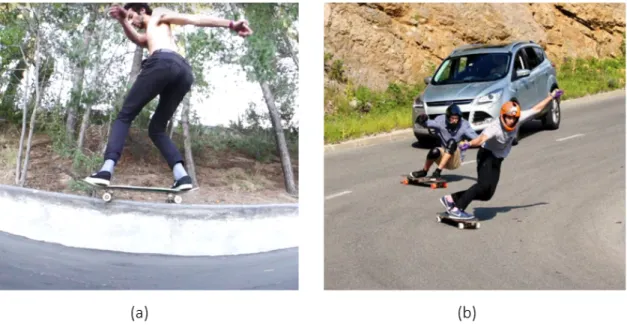
3.3 Detection results for Weakly-supervised temporal Activity Localization and Classification [10]. ’Act’ represents the temporal activations obtained from the final layer where ’Det.’ represents the detection obtained after thresh-olding the activations. ’GT’ represents the ground truth. . . 22 4.1 Example of bias in human annotations. The action category to be labeled is

skateboarding. (a) shows the action of skateboarding with a ”not fully locked in” feature where (b) shows a longboarder going down a hill. Given a human annotator does not know the differences between (a) and (b), a dataset for the action skateboarding would have a bias towards longboarding videos. . . 25 4.2 Frames from videos in the diving category for the test and train set. (a) shows

an example of ”diving” in Thumos14. (b) shows an example of ”diving” found online. The ambiguity of the term ”diving” returns videos of two separate actions. This shows to be a challenge with using keywords to search for videos when the action can be ambiguous. . . 34 4.3 Detections from I3D Features ”I3DF” and I3D Features with 95%

rerank-ing ”I3DF95%” and ground truth ”GT”. Two videos from the Thumos14 dataset are shown. For the Shotput video, I3DF95% does not detect the followthrough of the throw when the ball left the frame. Also, it can be seen that I3DF misses detections that are clear shotput actions. In the Frisbee Catch video, when the frisbee is left in the air with no human in frame, I3DF95% does not detect this as a Frisbee Catch. The ground truth also labels many temporal segments as a Frisbee Catch, with the throw in the segment. The detections here show the effectiveness of reranking for certain videos. . . 36

(13)

List of Tables

3.1 Detection performance comparisons over the Thumos14 dataset. UNTF and I3DF are abbreviations for UntrimmedNet features and I3D features, respec-tively. The ↓ symbol represents models that are trained with only the 20 classes that have temporal annotations, but without using their temporal annotations. . . 23 4.1 Detection performance comparisons using the online web video dataset. RNF

and I3DF are abbreviations for ResNet50 features and I3D features, respec-tively. The ↓ symbol represents models that are trained with only the 20 classes that have temporal annotations, but without using their temporal annotations. . . 32 4.2 Detection performance comparisons with re-ranking the online web video

dataset. RNF and I3DF are abbreviations for ResNet50 features and I3D features, respectively. The↓ symbol represents models that are trained with only the 20 classes that have temporal annotations, but without using their temporal annotations. It is shown that a 2% increase of detection perfor-mance resulted from the re-ranking with I3DF. . . 38

(14)

Chapter 1

Introduction

The purpose of human activity recognition is to automatically analyze ongoing activities from unknown videos. Given continuous videos, activity recognition must be able to detect starting and ending times of all activities within an inputted video. Being able to recognize complex human activities in continuous videos creates several important applica-tions [1], such as abnormality and suspicious activity detection in public places like subway stations and airports. Human activity recognition also allows for real-time monitoring of patients and elderly persons.

Human activities can be conceptually categorized into four different levels: ges-tures, actions, interactions, and group activities. Gestures are the individual movement of a specific body part. “Raising an arm” and “lifting a leg” are examples of gestures. Actions are activities that can consist of multiple gestures as “running,” “lifting,” and “waving”. Interactions involve activities with two or more persons and/or objects such as “a person stealing from another” or “two people fighting”. Lastly, group activities are made up of

(15)

conceptual groups involving multiple persons and/or objects. Group activities examples are “a group meeting,” “a group of people working,” “a group of people fighting.”

Activity recognition can be categorized into two different methodologies: single-layer approaches and hierarchical approaches. Single-single-layered approaches recognize human activities directly from a given sequence of images. This approach is best for the recognition of gestures and actions. Hierarchical approaches can recognize high-level human activities by putting together recognized simpler activities. This approach can recognize more com-plex activities. Being able to recognize activities in continuous videos, most single-layered approaches have adopted a sliding window method that can classify all possible subse-quences. The single-layered approach is the most effective in continuous videos where an activity can be captured from training sequences and can classify a particular sequential pattern. Single-layered approaches can be categorized into two classes: space-time and sequential approaches. Space-time approaches use a 3-D volume in the space-time dimen-sion to model a human activity. The volume is a concatenation of frames along the time axis. With the sequential approach, human activity is treated as a sequence of particular observations. This is done by obtaining a sequence of feature vectors that are extracted from images. With the extracted features, the sequential approach measures the likelihood between the sequence and the activity class, which then can classify the sequence with the corresponding activity.

Activity detection in continuous videos has posed to be a complicated problem, which requires both the classification and localization of activities in time. Classifying activities from temporal segments generated by sliding windows was considered a past

(16)

state-of-the-art approach [2] [3]. One of the drawbacks of this approach, however, is that sliding windows are exhaustive and lead to poor computational efficiency. Sliding window models are also not good at predicting flexible activity boundaries. Other works have looked into using an external ”proposal” generation mechanism [4]. These approaches all share a similar drawback: they do not learn deep representations in an end to end fashion but depend on deep features like VGG [6] and ResNet [7], etc. learned separately on image and video classification. The Region Convolutional 3D Network (R-C3D) remedies this issue with an end-to-end trainable model and learns task-dependent convolutional features [5]. R-C3D first computes fully-convolutional 3D ConvNet features, which can take in videos of various lengths. A feature map Cconv5b ∈ R512×

L

8×

H

16×

W

16 is produced from a network,

whereLis the number of frames, withH andW being the height and width of each frame, respectively. The next step of this network is the Temporal Proposal Subnet. This subnet uses anchor segments as predictors along the temporal axis, given labels of ground truth temporal segments for training. These proposed regions are then passed into a classification subnet to label the activity. A portrayal of the network is given in Figure 1.1.

The R-C3D requires labeled temporal segments for all training videos in a fully supervised setting. In the fully supervised setting, labels are given at the frame-wise level. An issue with this, however, is that being able to acquire such precise frame-wise annotations requires a significant amount of manual labor. With a growing number of activity categories and cameras, this would not scale efficiently. It is more feasible however for a person to give a few labels which encapsulate the contents of the video as a whole. Videos found on the internet are usually given with a few keywords that provide semantic discrimination. These

(17)

Figure 1.1: Region Convolutional 3D Network (R-C3D) [5]. 3D filters encode the frames, classifies proposal segments, and then pools features together.

types of video-level labels are termed as weak labels. These weak labels could be utilized to learn models that can classify and localize activities in a continuous video.

(18)

Chapter 2

Weakly-supervised Learning

2.1

Weak Supervision

In computer vision, weakly-supervised learning has been useful for several appli-cations. In [8], a pre-trained Convolutional Neural Network (CNN) is used to help detect regions in the output layer. The last pooling layer was replaced with a layer that imple-mented spatial pyramid pooling (SPP). This resulted in a function which takes in an input imagexand a region (bounding box)Rand produces a feature vector φ(x;R). The regions are generated by different region proposal schemes. The network then has two data streams, one for classification of the image, and the other for detection. The classification scheme takes in the regions, and performs classification on the individual regions, by mapping them to a C-dimensional vector of class scores. The detection stream takes in the same input, but this time compares the classes independently and scores the different regions per class. Thus, the first stream branch predicts which class each region is associated with, while the second branch selects which regions are most likely to contain informative image

(19)

frag-ments. Given the output of the classification streamσclass(xc)∈RC×|R| and the detection stream σdet(xd) ∈RC×|R|, the element-wise product xR=σclass(xc)σdet(xd) is taken to

achieve the final score. The computed region-level scores xR are then transformed to class prediction score by summation over the regions:

yc=

|R|

X

r=1

x|R|_cr (2.1)

This image-level class prediction scoreycis used compared with the image-level labels, the

weak labels, in this case, to evaluate the model. The model is shown in Figure 2.1.

Figure 2.1: Weakly Supervised Deep Detection Network [8]. CNN is pre-trained with ImageNet then region proposals are generated. The proposals are the branched off into two separate branches, one for detection and the other for recognition.

Including object detection, there have been other works utilizing weak labels for learning models, such as semantic segmentation [43] [44], visual tracking [45], reconstruc-tion [46], and so on. Within this domain, several works utilize the techniques of Multiple

(20)

Instance Learning (MIL) [9]. MIL is a type of supervised learning, where instead of given individual labeled instances, the learner receives a set of labeled bags. In the case of binary classification, a bag is labeled positive if at least one instance in the bag is positive, and negative if none of the instances are positive. MIL has been used due to the similarity of the structure of information as weak labels.

Compared to weak object detection, temporal localization with weak labels is a much more challenging task. The reason for this is the additional variation in content and length along the temporal axis of the video. This portion will introduce the framework for Weakly-supervised Temporal Activity Localization and Classification (W-TALC). With W-TALC [10], only the labels for the entire video are given, which needs to be processed at once. There is a natural tradeoff between the performance and computation for long videos. Processing long videos at fine temporal granularity may have significant memory and computation cost. However, coarse temporal processing could reduce the detection of granularity. With this trade-off in mind, the W-TALC paper asks: is it possible to utilize these networks just as feature extractors and develop a framework for weakly-supervised activity localization which learns only the task-specific parameters, thus scaling up to long videos and processing them at fine temporal granularity? W-TALC utilizes pair-wise video similarity constraints using an attention-based mechanism along with multiple instances learning to learn only task-specific parameters.

(21)

2.2

Related Works to W-TALC

There have been works that are closely related to W-TALC. The works in [11] focuses on utilizing weakly supervised data for action localization in sports videos. The work has a training set of sports video clips, where each clip has a given activity label performed by a player. This paper focuses on being able to identify which people in the clip are performing the given actions. They start by first running a player detector from Faster-RCNN [12] to obtain the top K persons detected, xik_i₌₁, from each frame. Since

frame-wise annotations are not given, action labels should be inferred within the training. Since this network is aimed towards looking for an action from a specific player, one player should have a high action category score, while others in the frame should not. Given this prior knowledge, the loss function for the new weakly-supervised loss is given as:

F =X f min i loss(xi, af) + X j6=i loss(xj, bg) (2.2)

where f denotes the frame,af as its corresponding action class, loss(xi, af) is the

loss of thei-th detection for action classaf, andloss(xj, bg) is the loss for thej-th detection

for the background class. The loss here is given as:

loss(xi, af) =−log(sof tmax(CN Na(xi, af))) (2.3)

where CN Na(xi, af) is the predicted score for action class af after feeding the

detection xi into the network. The softmax is used for normalizing scores across all

cat-egories. For back-propagation, error gradients are computed by inferring which detected person should be assigned the category class. The rest of the detected persons are as-signed as background labels. The background labels, in this case, are equally as important

(22)

Figure 2.2: Weakly-supervised Attention Models for Action Localization in Video [11]. First player detection is performed with Faster-RCNN. For each frame, one person should be classified as an action, while the remaining detections are labeled as background. Labels of the player are not given during training and must be inferred during learning.

because they give information to what the category class shouldn’t be. In the weakly su-pervised case, the background labels are very important because background classes are shared across all categories, which allow the network to find the real person in the category class. One important implementation that came from this paper is the use of the temporal attention model. Analyzing the video frame by frame and passing it through the classi-fier can negatively affect the learning. This is because the weakly-supervised portion of this model depends on an action being performed in a frame, and learns by differentiating it from the background classes, in this case, other players not performing the action. It is not given that every frame will contain an action within all the action categories, and so if the model must choose one player as a positive example, this can result in negative performance. Given this, the paper introduces the temporal attention model. This model assigns a weight to every frame in a clip. During the training process, the model assigns

(23)

frames with low weights that have a high error, and high weights with frames that have low errors. This allows the model to slowly learn the relevant frames that contain actions within the current video. The attention value is computed for each frame, then normalized along the temporal dimension with a softmax operator. The temporal attention model is an important resource for weakly-labeled video for detection along the temporal dimension. This allows the overall network to learn and focus on training with frames or segments that are more likely to contain the action category.

Figure 2.3: Finding Actors and Actions in Movies [17]. Framework for using actor/action label scripts for weakly supervised learning. Figure shown is the results of automatic de-tection and annotation of actions and characters in the movie Casablanca.

Other works of literature focus on using scripts or subtitles as weak labels for activity localization. In [17], scripts that contain actor/action pairs are used as weak labels for constraints in a discriminative clustering framework. Faces are automatically extracted

(24)

to recognize people and a framework is used to learn the names of characters in movies. Then the joint actor/action constraint is used to demonstrate the advantage of weakly-supervised action learning. In [18], subtitles are searched for texts that are related to human actions. These texts are used for coarse temporal localization of actions for training. W-TALC differs in this sense because the only information needed per video is a single label for the entire video, instead of having multiple labels throughout the temporal region.

Figure 2.4: Weakly Supervised Action Learning with RNN based Fine-to-coarse Modeling [19]. Framework for using initial segmentation generated by uniform segmentation. Then a RNN fine-to-coarse system is iteratively trained to align frames to respective actions.

Few works focus on using the temporal ordering of actions for localization [20] [21]. These works are similar to weak supervision in that it does not need frame-wise labels of a given action, rather than an action follows a sequential set of sub-actions within the video. An example of this would be a video of making tea. The sub-actions for this might include

(25)

getting a cup, putting a teabag inside, and pouring hot water. In [19], the authors iteratively train and realign activity regions using a Recurrent Neural Network (RNN). Given a list of ordered actions per video, an initial segmentation is generated and using a fine-to-coarse system, frames are aligned to respective actions. How W-TALC differs is that information about the order of the activity is not needed for training.

(26)

Chapter 3

Model Description

3.1

Introduction

This chapter summarizes the work done in [10]. The work in [10] is used as the main model for this thesis. Consider a training set of n videos X =xi n_i₌₁ with variable temporal durations denoted byL=li

n

i=1 (after feature extraction) and activity label set

A= ai n i=1 whereai= xj_i mi

i=1are themi(≥1) labels for thei

th_{video. The set of activity}

categories is defined as S =

∪

n i

i=1 ai =

ai n_i₌₁c . During testing, given a video x, we need

to predict a set xdet =

(sj, ej, cj, pj) n(x)

i=1, where n(x) is the number of detections for x. sj, ej are the start time and end time of thejthdetection,cj represents its predicted activity

category with confidence pj. With these notations, the proposed framework is presented

(27)

Figure 3.1: Framework for Weakly-supervised temporal Activity Localization and Classi-fication [10]. Frames are passed through a feature extractor which derives the RGB and Optical Flow streams. The feature vectors are then concatenated and passed through a FullyConnected-ReLU-Dropout operation. This is then passed through a label-space pro-jection which then computes two separate loss functions: Multiple Instance Learning Loss and Co-Activity Similarity Loss.

3.2

Feature Extraction

W-TALC uses two feature extractors: UntrimmedNet Features [14] and I3D Fea-tures [13]. UntrimmedNet feature extractor consists of an RGB stream and an Optical Flow stream. The RGB stream is fed with one frame, where the Optical Flow stream is fed 5 frames. The network used is pre-trained on ImageNet. I3D network also has both RGB and Optical Flow streams of non-overlapping 16 frame groups. The output of the network is a feature vector of dimension 1024 for each of the two streams.

After the feature extraction process, each video xi is represented by matrices Xri

and Xo_i, which denote the RGB and optical flow features, respectively. These features are both of dimension 1024 x li, where li is dependent on both the video index i and also the

feature extraction process used. These features become the input to the weakly-supervised learning module.

(28)

seconds to over an hour. Since in this weakly-supervised method, we are given a label for the entire video, so the entire video must be processed at once. GPU memory constraints become an issue for very long videos. To preserve the granularity of localization for the videos, the entire video is processed if the length is less than a pre-defined length T. If the length of the video, however, is greater than T, a random section of the clip of length T is extracted instead. This allows the frames to be contiguous while meeting the GPU bandwidth constraints.

3.3

Fully Connected Layer

A fully connected layer is introduced followed by ReLU and Dropout on the ex-tracted features. The operation for video with index i can be formalized as follows.

Xi=D(max(0,Wfc " Xr_i Xo_i # ⊕bf c), kp) (3.1)

whereDrepresents DROPOUT with kp representing its keep probability,⊕is the addition

with broadcasting operator, Wf c ∈ R2048x2048 and b ∈ R2048x1 are the parameters to be learned from the training data andXi ∈R2048×li _{is the output feature matrix for the entire} video.

3.4

Label Space Projection

For each video i we are given a feature representation Xi. This representation is

used to classify and localize activities in the videos. Xi is projected into the label space

(29)

obtained can be represented as below.

Ai=WaXi⊕ba (3.2)

The class-wise activations shown represent the possibility of each activity at the given temporal instants. The activations are used for computing the loss functions presented later.

3.5

k

-max Multiple Instance Learning

The weakly-supervised activity localization and classification problem is related to Multiple Instance Learning. With MIL, all samples can be grouped into two bags, one positive and one negative. A bag is labeled positive if at least one positive instance occurs and labeled negative if no positive instances are contained. The bags are used as training data to learn the model. In this case, an entire video can be seen as a bag of instances, where each instance is a feature vector at a certain time. Using these instances, the activation score can be calculated as the average of k-max activation over the temporal dimension for a given category. ki=max 1,li s (3.3)

where k is set proportionally to the number of elements in the bag and s is a design parameter. From here the class-wise confidence score for category j video i can be shown by, sj_i = 1 ki max M⊂Ai[j,:] |M|=ki ki X l=1 Ml (3.4)

(30)

where M is the set that contains l elements. A softmax non-linearity is then applied to obtain the probability mass function over the categories. To compute the Multiple Instance Learning Loss (MILL), the probability mass function is compared to the ground truth distribution. Given the predicted probability mass function pi and the ground truth label

vector, the MILL is then the cross-entropy of the two as follows,

LMILL = 1 n n X i=1 nc X j=1 −yj_ilog(pj_i) (3.5)

wherepj_i represents the probability mass function over all the categories, andyi= [y1i, ..., y nc

i ]T

is the normalized ground truth vector.

3.6

Co-Activity Similarity

W-TALC focuses on finding correlations between videos of similar categories. Let

Sj be the set of all training videos in the jth category, with activityaj as one of its labels.

Ideally, a pair of videos belonging to the setS_j should have similar feature representations in the instance where activity aj occurs. Also, given the same video pair, the feature

representation of one video where aj occurs should be different in another video where aj

does not occur. This is not directly enforced in MILL. Because of this, the introduction of Co-Activity Similarity Loss (CASL) is given. Since frame-wise labels are not given, class-wise activations are needed to learn the activity portions of the videos. CASL helps to learn the feature representation while simultaneously learning the label space projection. First, the per-video class-wise activation scores are normalized along the temporal axis with

(31)

softmax non-linearity as below: ˆ A_i[j, t] = exp( ˆAi[j, t]) Pli t0₌₁exp( ˆAi[j, t0]) (3.6)

where t indicates the time instances and j indicates the current category. This above is referred to as attention, as it relates to the sections of the video where an activity occurs in a certain category. When the attention has a high value for a particular category, there is a high occurrence-probability that the category action has occurred. CASL depends on the attention scores to determine class-wise feature vectors that have regions of high and low occurrence-probability as shown:

H_fj i =XiAi[j,:]T (3.7) L_fj i = 1 li −Xi(1−Aˆi[j,:]T) (3.8)

whereHfj_i and Hfj_i represents the high and low attention regions aggregated feature repre-sentations respectively for video i for category j. Cosine similarity is used to measure the degree of similarity between two feature vectors as below:

d[fi,fj] = 1− hfi,fji hfi,fii 1 2hf_j,f_ji 1 2 (3.9)

As discussed earlier, a pair of videos belonging to the same set Sj should have similar feature representations in the portion where aj occurs. Also, the same video pair should

have different feature representations where aj occurs in one video and where aj doesn’t

occur in the other. To enforce these properties, ranking hinge loss was used as follows:

Lmn_j = 1 2 max(0, d[Hfj_m,Hfj_n]−d[Hfj_m,Lfj_n] +δ) +max(0, d[Hfj_m,Hfj_n]−d[Lfj_m,Hfj_n] +δ) (3.10)

(32)

whereδis the margin parameter, which is set to 0.5 for these experiments. The two terms in the loss function above have equivalent meaning. Essentially, high attention region features in both videos should have more similarity than high attention region features in one video and low attention region feature in the other video. So when the two high attention region features have a much higher cosine similarity, given equation 3.10, d[Hfj_m,Hfj_n] will become smaller, and thus the loss will decrease. The total loss for the entire training set can be shown as: L_CASL = 1 nc nc X j=1 1 |Sj| 2 X xm,xn∈Sj Lmn_j (3.11)

3.7

Optimization

To learn the weights of the weakly-supervised layer, the total loss is given as follows:

L=λLM ILL+ (1−λ)LCASL+α||W||2F (3.12)

where W are the weights to be learned in the network. In this experiment, λ= 0.5 and α = 5×10−4. The loss above is optimized using Adam [47] with a batch size of 10. Each batch is created in a way where at least three pairs of videos each have at least one pair within the same category.

3.8

Experiments

For W-TALC, two datasets were used: ActivityNet v1.2 [22] and Thumos14 [23]. Both of these datasets include untrimmed videos with frame-wise labels of actions along the temporal dimension. Because W-TALC is weakly-supervised, only the label of an entire

(33)

video is used for training, where the frame-wise labels are used for the test set. ActivityNet v1.2 contains 4819 videos for training, 2383 videos for validation and 2480 videos for testing. The frame-wise labels were withheld from the training set. There is a total of 100 classes with an average of 1.5 temporal activity segments per video. Training videos are used to train the network, where the validation set is used for testing. The Thumos14 dataset contains 1010 videos for validation and 1574 videos for testing. Among these videos, there are 200 validation videos and 213 test videos that contain temporal annotations. Thumos14 has a total of 101 categories, with an average of 15.5 activity temporal segments per video. Among the 101 categories, 20 categories have temporal annotations. Although Thumos14 is a much smaller dataset than ActivityNet v1.2, the temporal labels within Thumos14 are very precise and contain several videos with multiple activities occurring. This makes the dataset much more challenging. Also, the lesser number of videos contained in Thumos14 makes it even more challenging to efficiently learn the weakly-supervised network.

Feature extractors are not finetuned and weights are initialized for the weakly-supervised layers by Xavier method [24]. The network is trained on a single Tesla K80 GPU using TensorFlow, with the design parameters= 8 for both datasets.

Mean average precision (mAP) is used to compute the classification performance. From Table 1, W-TALC performs significantly better than other state-of-the-art approaches. Jointly optimizing with loss functions MILL and CASL shows better performance than only using MILL. With only using MILL, i.e. λ= 1.0, a 7-8% decrease in mAP occurs compared to using both MILL and CASL. This shows that the introduction of CASL has a significant benefit with this framework.

(34)

Figure 3.2: Charts from [10]. (a) Shows diffeernt detection performances with Thumos14 by changing weights on MILL and CASL. Higherλ means more weight on MILL and vice versa. (b) shows changes of the detection performance by varying the maximum possible length of video sequences during training.

Since only the labels of the entire video are given, entire videos need to be processed at once to compute the loss functions. Videos may be extremely long, which would cause difficulties meeting GPU memory constraints.

To meet these constraints, a pre-defined length T is used to maintain the length of the videos in this batch size. Given this strategy, long length videos can be processed at once. This will also act as a data augmentation technique since the video is randomly cropped along the temporal axis to make it a fixed-length sequence. Using a lower T value will decrease computation time. The disadvantage to this, however, is that errors will be introduced in the labels of a training batch. There is a natural tradeoff between the performance and the computation time. For this study, T = 320swas chosen to be a reasonable value for the detection performance to reach a plateau.

(35)

Figure 3.3: Detection results for Weakly-supervised temporal Activity Localization and Classification [10]. ’Act’ represents the temporal activations obtained from the final layer where ’Det.’ represents the detection obtained after thresholding the activations. ’GT’ represents the ground truth.

and video classification with only video-level labels. The paper presents a novel Co-Activity Similarity loss. This loss was shown to be complementary to the Multiple Instance Learn-ing Loss. This paper also presented a method for processLearn-ing long length videos, while being able to process them at high granularity. Using two challenging datasets, this paper achieves state-of-the-art results with the weakly-supervised temporal activity localization

(36)

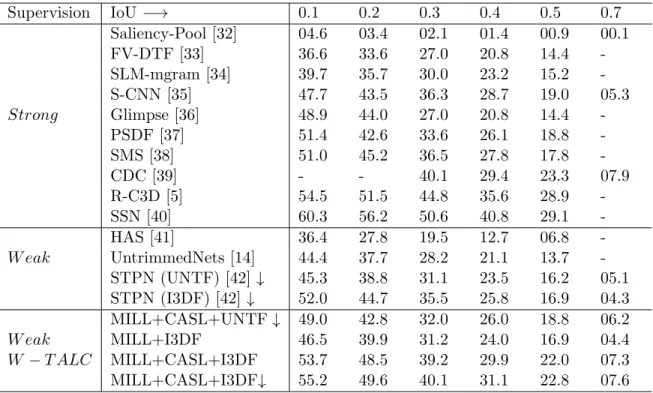
and classification problem. Supervision IoU −→ 0.1 0.2 0.3 0.4 0.5 0.7 Saliency-Pool [32] 04.6 03.4 02.1 01.4 00.9 00.1 FV-DTF [33] 36.6 33.6 27.0 20.8 14.4 -SLM-mgram [34] 39.7 35.7 30.0 23.2 15.2 -S-CNN [35] 47.7 43.5 36.3 28.7 19.0 05.3 Strong Glimpse [36] 48.9 44.0 27.0 20.8 14.4 -PSDF [37] 51.4 42.6 33.6 26.1 18.8 -SMS [38] 51.0 45.2 36.5 27.8 17.8 -CDC [39] - - 40.1 29.4 23.3 07.9 R-C3D [5] 54.5 51.5 44.8 35.6 28.9 -SSN [40] 60.3 56.2 50.6 40.8 29.1 -HAS [41] 36.4 27.8 19.5 12.7 06.8 -W eak UntrimmedNets [14] 44.4 37.7 28.2 21.1 13.7 -STPN (UNTF) [42] ↓ 45.3 38.8 31.1 23.5 16.2 05.1 STPN (I3DF) [42]↓ 52.0 44.7 35.5 25.8 16.9 04.3 MILL+CASL+UNTF↓ 49.0 42.8 32.0 26.0 18.8 06.2 W eak MILL+I3DF 46.5 39.9 31.2 24.0 16.9 04.4 W −T ALC MILL+CASL+I3DF 53.7 48.5 39.2 29.9 22.0 07.3 MILL+CASL+I3DF↓ 55.2 49.6 40.1 31.1 22.8 07.6 Table 3.1: Detection performance comparisons over the Thumos14 dataset. UNTF and I3DF are abbreviations for UntrimmedNet features and I3D features, respectively. The

↓ symbol represents models that are trained with only the 20 classes that have temporal annotations, but without using their temporal annotations.

(37)

Chapter 4

Weakly-supervised Learning from

Web Videos

4.1

Web videos

Popular datasets such as Thumos14 has allowed for action recognition and tempo-ral localization across many numbers of classes. The W-TALC model allowed for weakly-supervised learning to classify videos and detect actions along the temporal dimension. Supervised learning methods have been very effective given only labels of the videos, how-ever being able to fully annotate actions in videos at a large scale would require enormous manual labor. Video sharing sites such as YouTube have grown significantly and are rich sources for video datasets. This brings the question of whether action keywords can be used to scrape videos online, and then be used as a training set for W-TALC?

(38)

Figure 4.1: Example of bias in human annotations. The action category to be labeled is skateboarding. (a) shows the action of skateboarding with a ”not fully locked in” feature where (b) shows a longboarder going down a hill. Given a human annotator does not know the differences between (a) and (b), a dataset for the action skateboarding would have a bias towards longboarding videos.

images for learning [26] [27] [28]. Recently, there have been many works that focus on video summarization, where the goal is to process long videos and being able to extract the action found within the video. These methods have looked towards summarizing videos in an unsupervised manner [29] [30] [31]. Consider an example video of skateboarding, being blind to the video category, it would be difficult to segment out the corresponding features of skateboarding i.e. ollie, slides, grinds that are not fully locked in, etc. Being able to learn these specific features in a fully supervised setting would require enormous amounts of human-labeled data for video-action pairs along the temporal dimension. Collecting labeled time data is difficult to find using only web videos. Also, if manual annotations of videos were to be an approach, only a limited number of users would be annotating the training videos, which could possibly lead to a bias in the summarization model.

(39)

Collecting videos with only the entire label of a video is much easier however since most videos online are associated with some tags. There have been works into whether weakly-supervised learning can be achieved with only video-level annotation for summa-rizing web videos [16]. Some datasets that contain video level tags include YouTube-8M [25], which contains 237k human-verified segment labels, with 1000 classes, and 5.0 average segments per video. These are reliable datasets for training, however, we are still limited in our ability to freely search for web videos within our desired classes. We pose an important question in this work: Can we train the Weakly-supervised Temporal Activity Localization and Classification network given only searched web videos?

4.2

YouTube Data API

For video sharing sites, YouTube was chosen because of its large number of on-line videos and its YouTube Data API so additional features can be entered for scraping videos. The results of this online video dataset are to be compared with the results of the Thumos14 dataset. We want to see if only keywords can be used for creating a video dataset online and be used to localize and classify videos. This is similar to the use of the Thumos14 dataset, except without the full supervision of the video-level labels. The 20 classes of the Thumos14 reduced dataset is used as our actions because of its available temporal annotations in its test set, which will be used for comparing the online video dataset versus the Thumos14 dataset for training. YouTube Data API allows for a variety of features to be added to better specify the user’s query. Since there are almost an endless amount of specifications for querying videos online, the only features this dataset uses for its

(40)

search is the action keyword itself. These action keywords include ”BaseballPitch”, ”Basket-ballDunk”, ”Billiards”, ”CleanAndJerk”, ”CliffDiving”, ”CricketBowling”, ”CricketShot”, ”Diving”, ”FrisbeeCatch”, ”GolfSwing”, ”HammerThrow”, ”HighJump”, ”JavelinThrow”, ”LongJump”, ”PoleVault”, ”Shotput”, ”SoccerPenalty”, ”TennisSwing”, ”ThrowDiscus”, ”VolleyballSpiking”. The evaluation here is how well does the keyword obtains video data related to itself.

Since using YouTube Data API could be resourcefully expensive, credentials were needed to access the API. Requesting credentials gives the user a server key, which keeps track of the user’s API access, quota, and reports. For each of the twenty categories, we wanted 100 videos per category, totaling 2000 videos. We wanted the video lengths to contain short clips, and long clips to add variety to the types of videos we received. The API allowed users to search for videos not within specific time lengths, but pre-defined time blocks. This included videos within ”short” durations, which were videos less than four minutes, and ”medium” durations, which were videos between four and twenty minutes. For each category, 50 of the videos were searched within the short category and the other half with the medium category. Each user is given a daily quota limit of 10,000 units per day. The goal was to search and download 2000 videos with YouTube’s Data API at once while staying under the daily quota limit. For each search query, the user receives 50 videos per search, costing 100 units each. The 50 videos returned are the first 50 videos on page one of the keywords searched. To search for more videos, the user must use the returned next page token to run another search, which will give another 50 videos returned. Since some videos are duplicated on the next page, and other videos are not allowed for download,

(41)

each category searched for 2 pages of short videos, and 2 pages of medium videos. This becomes a total of 200 videos per category, at a cost of 400 quota units. For 20 categories this equates to 8000 quota units, under the 10,000 units limit. After downloading all the videos, the top 50 returned results from the short videos, and the medium videos are used as the 100 total videos per category. These top 100 videos exclude duplicate videos found between the first and second page of a search.

4.3

Feature Extraction

After downloading all the videos for the training set, frames needed to be extracted for later feature extraction. The frames were extracted from each video at 25 frames per second and rescaled to 224x224 dimensions using a shell script. The frames were extracted for the YouTube downloaded dataset videos, as well as the Thumos14 test set videos. After extracting the frames of all the videos, feature extraction of each image needs to be per-formed. Two different feature extractors are used for this experiment: ResNet50 [7] and I3D [13].

4.3.1 Deep Residual Network

Deep residual learning overcomes the challenge of training deeper neural networks. Deep convolutional neural networks led to groundbreaking results for image classification. When deeper networks were able to start converging, there was a problem of degradation. As the network became deeper, the accuracy saturates and then degrades rapidly. This previous issue was thought to be caused by overfitting, however, this was not the case. The

(42)

paper hypothesized that if earlier in the layers an underlying mapping was optimal, the network should have no problem simply performing identity mapping throughout the rest of the layers. The degradation problem, however, shows that these deeper networks have difficulties converging to this underlying mapping. Deep residual learning lets layers instead fit a residual mapping. Consider an underlying mappingH(x) fit by only a few top layers, wherexdenotes the input to the first layer. Rather than stack layers to approximateH(x), the layers instead approximate a residual function F(x) :=H(x). Since deeper layers have difficulties converging to identity mappings, in this case, if an identity mapping is optimal, the layers simply are driven to zero. This residual network overcomes the degradation problem and allows for deeper networks to converge to these identity mappings. The residual network used for this experiment is a ResNets network of 50 layers (ResNet50). This is a deeper network which is modified with a bottleneck design. Each F stacks 3 layers of 1x1, 3x3, and 1x1 convolutions, where the 1x1 layers reduce and restore the original dimensions. Given that x and F are not the same dimension, a linear projection Ws is performed by

the shortcut connection:

y=F(x,

Wi ) +Ws(x) (4.1)

whereF(x,

Wi ) is the residual mapping to be learned.

4.3.2 Two-Stream Inflated 3D ConvNet

The second feature extractor used is the Two-Stream Inflated 3D ConvNet (I3D). I3D is created by simply converting 2D classification models into 3D ConvNets. This is created by inflating all the filters and pooling kernels, which gives them an additional

(43)

temporal dimension. Given a typical square filter in 2D N ×N, the filter is inflated to 3DN ×N ×N. Parameters from the pre-trained ImageNet models are also bootstrapped across the new temporal dimension. This is done by repeating weights of the 2D filters N times across the new dimension, and rescaling by dividing byN. This is so the convolution filter response is the same. In a two-dimensional spatial image, pooling kernels and strides have symmetric receptive fields, so features deeper in the network are equally affected by image locations far away. Within the temporal dimension, however, symmetric receptive fields are not necessarily optimal. If the receptive field grows too quickly, then features from different objects could break early detected features. On the other hand, if it grows too slowly, scene dynamics may not be captured well. Through experimentation, I3D does not perform temporal pooling in the first two max-pooling layers of Inception-v1. The model is trained on 64 frame snippets and tested on entire videos. The 3D ConvNet also keeps a two-stream configuration, one I3D network trained on RGB inputs, and the other on flow inputs. The two networks are trained separately, and their predictions are averaged. The I3D model is pre-trained on Kinetics dataset, and considerably improves the state-of-the-art action classification reaching98.0% on theUCF-101 dataset. To extract features from the I3D model, RGB video frames and optical flow is extracted from the videos. TV-L1 optical flow is used as the optical flow estimation as it is the same one used in W-TALC.

4.4

Experimentation

Thumos14 test set was used for evaluating our web video-based training. Thu-mos14 includes untrimmed videos with frame-wise labels of actions along the temporal

(44)

dimension. The Thumos14 dataset contains 1010 videos for validation and 1574 videos for testing. Among these videos, there are 200 validation videos and 213 test videos that contain temporal annotations. Thumos14 has a total of 101 categories, with an average of 15.5 activity temporal segments per video. Among the 101 categories, 20 categories have temporal annotations. The temporal labels within Thumos14 are very precise and contain several videos with multiple activities occurring. For testing, 213 test videos were used that belonged to the 20 categories with temporal annotations. This makes Thumos14 stringent testing set for our web video-based training. The network is trained on a single Tesla K80 GPU, with the design parameters= 8.

4.5

Results

Table 4.1 shows the results for training the W-TALC network with web videos. The ResNet50 extracted features have fairly poor performance compared to other strong and weakly supervised methods. Performance with using I3D features, however, shows a much better performance. An analysis of the online web video dataset is discussed in the next section.

4.6

Noisy data

Taking a closer look at the online video dataset, there were plenty of noisy videos that did not correspond to the activity class. This was presumed to be an issue, so each of the 2000 videos were inspected to see whether they related to the category class or

(45)

Supervision IoU −→ 0.1 0.2 0.3 0.4 0.5 0.7 Saliency-Pool [32] 04.6 03.4 02.1 01.4 00.9 00.1 FV-DTF [33] 36.6 33.6 27.0 20.8 14.4 -SLM-mgram [34] 39.7 35.7 30.0 23.2 15.2 -S-CNN [35] 47.7 43.5 36.3 28.7 19.0 05.3 Strong Glimpse [36] 48.9 44.0 27.0 20.8 14.4 -PSDF [37] 51.4 42.6 33.6 26.1 18.8 -SMS [38] 51.0 45.2 36.5 27.8 17.8 -CDC [39] - - 40.1 29.4 23.3 07.9 R-C3D [5] 54.5 51.5 44.8 35.6 28.9 -SSN [40] 60.3 56.2 50.6 40.8 29.1 -HAS [41] 36.4 27.8 19.5 12.7 06.8 -W eak UntrimmedNets [14] 44.4 37.7 28.2 21.1 13.7 -STPN (UNTF) [42] ↓ 45.3 38.8 31.1 23.5 16.2 05.1 STPN (I3DF) [42]↓ 52.0 44.7 35.5 25.8 16.9 04.3 MILL+CASL+UNTF ↓ 49.0 42.8 32.0 26.0 18.8 06.2 W eak MILL+I3DF 46.5 39.9 31.2 24.0 16.9 04.4 W −T ALC MILL+CASL+I3DF 53.7 48.5 39.2 29.9 22.0 07.3 MILL+CASL+I3DF↓ 55.2 49.6 40.1 31.1 22.8 07.6 MILL+CASL+RNF ↓ 27.4 21.6 15.5 11.3 7.7 -Online MILL+CASL+I3DF(RGB)↓ 34.8 28.6 19.7 13.1 9.0 -Dataset MILL+CASL+I3DF↓ 37.5 31.6 23.2 15.9 11.6

-Table 4.1: Detection performance comparisons using the online web video dataset. RNF and I3DF are abbreviations for ResNet50 features and I3D features, respectively. The ↓

symbol represents models that are trained with only the 20 classes that have temporal annotations, but without using their temporal annotations.

not. There were some interesting results upon inspection. In almost all the video classes, some videos contained interviews of people talking about the class action, but no action is performed. Other noise included video games of the action itself, but not real human action. With the category ”Cricket Bowling”, there were a high number of videos that showed a cricket bowling machine, without the action itself included. This accounted for most of the action class. Another noise along all the actions were tutorial videos on how to perform the action, without the action shown itself in most. The largest noisy data within an action class was for the ”diving” category. The Thumos14 dataset considers the

(46)

action category ”diving” to involve jumping off a diving board as shown in Figure 4.7. The videos obtained online for this action class consisted primarily of deep-sea diving videos. The deep-sea diving videos were present in over 80% of the total diving category videos. This inspection allowed us to understand the slightly lower performance for the online video dataset. There were possible actions that could be taken to avoid these noisy videos. One would be to have a network classify whether a video is a tutorial or interview instead of an action. This would help clear a high majority of the videos. The other action would be to use more refined keyword choices, such as Olympic diving instead of only diving. These approaches would certainly increase the detection performance of the network; however, these refinements seem too customized for this dataset. We want a method that did not depend on knowing the noises and biases presented in the online video dataset. So, the question presented is whether there is a way to filter out noisy videos in a dataset given no prior knowledge about its distribution.

4.7

Reranking method

Given that most of the videos within an action category should be similar, we want to be able to see which videos within an action category are the least similar to the rest and score their total similarity. From these scores, we want to re-rank the videos and remove the topN lowest scored videos. W-TALC focuses on identifying correlations between videos of similar categories. For the reranking method used, we wanted to exploit the high attention learned from the network, which aggregates the video into a single feature vector and then use these aggregated vectors to compare with each other within its class.

(47)

Figure 4.2: Frames from videos in the diving category for the test and train set. (a) shows an example of ”diving” in Thumos14. (b) shows an example of ”diving” found online. The ambiguity of the term ”diving” returns videos of two separate actions. This shows to be a challenge with using keywords to search for videos when the action can be ambiguous.

After a full training on the video dataset, we want to project each video into a single vector for comparison. Each video xi is passed through the feature extraction

process. The new features are represented by matrices Xr_i and Xo_i which denote the RGB and optical flow features, respectively. Each extracted feature is passed through the trained fully connected layer as follows.

Xi=D(max(0,Wfc " Xr_i Xo_i # ⊕bf c), kp) (4.2)

whereDrepresents DROPOUT with kp representing its keep probability,⊕is the addition

with broadcasting operator, Wf c ∈ R2048x2048 and b ∈ R2048x1 are the parameters to be learned from the training data andXi ∈R2048×li is the output feature matrix for the entire video.

(48)

The feature representation Xi is then projected to the label space by

Ai=WaXi⊕ba (4.3)

with the weights and bias already learned. Now, the videos have probabilities of activities at each temporal instant. Utilizing the Co-Activity Similarity stream, first the per-video class-wise activation scores are normalized along the temporal axis with softmax non-linearity as: ˆ A_i[j, t] = exp( ˆAi[j, t]) Pli t0₌₁exp( ˆAi[j, t0]) (4.4)

where t indicates the time instances and j indicates the current category. This is now the attention matrix needed to finally transform our videos into a single feature vector for comparison. The attention should have a high value for portions of the video where an activity most likely occurs. Since the attention has already been learned, it should be able to pick out the portions of the videos that is relevant to the action class we are searching for. The final single feature vector per video is given as:

H_fj

i =XiAi[j,:]

T _(4.5)

where Hfj_i is the high attention regions aggregated feature representations respectively for videoi for categoryj. The features within the same categoryj should have high similarity, so the cosine similarity of feature vectorHfj_i is taken with all videos in categoryj. Then all the scores are added together and feature vectorHfj_i is scored based on the total similarity as below: d[Hfj_i] = N X k=0,k6=i hH_fj i,Hf j ki hH_fj i,Hf j ii 1 2_h_fj k,f j ki 1 2 (4.6)

(49)

whereN is equal to the total number of videos in category j. These scores are then ranked from lowest to highest score. Removing the lowest N videos for each feature extractor, the network was retrained from scratch and evaluated on the Thumos14 test set again.

Figure 4.3: Detections from I3D Features ”I3DF” and I3D Features with 95% reranking ”I3DF95%” and ground truth ”GT”. Two videos from the Thumos14 dataset are shown. For the Shotput video, I3DF95% does not detect the followthrough of the throw when the ball left the frame. Also, it can be seen that I3DF misses detections that are clear shotput actions. In the Frisbee Catch video, when the frisbee is left in the air with no human in frame, I3DF95% does not detect this as a Frisbee Catch. The ground truth also labels many temporal segments as a Frisbee Catch, with the throw in the segment. The detections here show the effectiveness of reranking for certain videos.

4.8

Results with Reranking

Table 4.2 shows the performance of our reranking method. With the Resnet50 features, the reranking method has a decrease in performance with the detection mAP. This is probably because the ResNet50 features have a poor performance on the classification portion of the videos, so the label space projection does a poor job of learning the relevant

(50)

time instants in each video. As it can be seen with the top 95% and top 90% of videos with ResNet50, the performance decreases. This means the videos being removed are relevant videos to the class category. The results on our reranking method with the I3D features show a small improvement for the detection mAP performance. Given the top 95% and 90% of videos with I3D, the detection mAP increased by 2%, which shows some notable significance with using the natural structure of the network for reranking. Using the top 80% of the videos, the performance equates to using the entire video dataset, which means it is starting to remove too many videos relevant to the action class.

(51)

Supervision IoU −→ 0.1 0.2 0.3 0.4 0.5 0.7 Saliency-Pool [32] 04.6 03.4 02.1 01.4 00.9 00.1 FV-DTF [33] 36.6 33.6 27.0 20.8 14.4 -SLM-mgram [34] 39.7 35.7 30.0 23.2 15.2 -S-CNN [35] 47.7 43.5 36.3 28.7 19.0 05.3 Strong Glimpse [36] 48.9 44.0 27.0 20.8 14.4 -PSDF [37] 51.4 42.6 33.6 26.1 18.8 -SMS [38] 51.0 45.2 36.5 27.8 17.8 -CDC [39] - - 40.1 29.4 23.3 07.9 R-C3D [5] 54.5 51.5 44.8 35.6 28.9 -SSN [40] 60.3 56.2 50.6 40.8 29.1 -HAS [41] 36.4 27.8 19.5 12.7 06.8 -W eak UntrimmedNets [14] 44.4 37.7 28.2 21.1 13.7 -STPN (UNTF) [42] ↓ 45.3 38.8 31.1 23.5 16.2 05.1 STPN (I3DF) [42]↓ 52.0 44.7 35.5 25.8 16.9 04.3 MILL+CASL+UNTF ↓ 49.0 42.8 32.0 26.0 18.8 06.2 W eak MILL+I3DF 46.5 39.9 31.2 24.0 16.9 04.4 W −T ALC MILL+CASL+I3DF 53.7 48.5 39.2 29.9 22.0 07.3 MILL+CASL+I3DF↓ 55.2 49.6 40.1 31.1 22.8 07.6 MILL+CASL+RNF ↓ 27.4 21.6 15.5 11.3 7.7 -W eak MILL+CASL+RNF95% ↓ 26.1 20.4 14.1 10.1 6.9 -W −T ALC MILL+CASL+RNF90% ↓ 25.6 20.3 14.6 10.5 7.2 -MILL+CASL+I3DF(RGB)↓ 34.8 28.6 19.7 13.1 9.0 -Online MILL+CASL+I3DF↓ 37.5 31.6 23.2 15.9 11.6 -Dataset MILL+CASL+I3DF95%↓ 39.5 33.8 24.3 16.1 11.2 -MILL+CASL+I3DF90%↓ 39.2 33.9 24.8 16.3 11.3 -MILL+CASL+I3DF80%↓ 37.7 32.1 23.6 16.2 11.4

-Table 4.2: Detection performance comparisons with re-ranking the online web video dataset. RNF and I3DF are abbreviations for ResNet50 features and I3D features, respectively. The

↓ symbol represents models that are trained with only the 20 classes that have temporal annotations, but without using their temporal annotations. It is shown that a 2% increase of detection performance resulted from the re-ranking with I3DF.

(52)

Chapter 5

Conclusions

This paper focuses on the work of Weakly-supervised Temporal Activity Local-ization and Classification using web videos. First, the YouTube Data API was used to download 2000 videos for training, containing the same 20 categories in the Thumos14 re-duced dataset. Only the keywords of the videos were used to search for videos. Feature vectors were extracted from the web videos using Resnet50 and I3D feature extractors. These features were used to train the W-TALC network and shows promising results for the use of web videos. The web videos were thoroughly searched to reveal some common bias and noise within the web videos. A re-ranking strategy is employed by exploiting the W-TALC network, which compresses each video into a single feature vector using the trained attention weights. The cosine similarity is calculated for each pair of videos within the same class and re-ranks videos according to this score. Retraining the W-TALC network from scratch with the reranked web videos show an increase in detection performance with the I3D features. This was able to demonstrate that given only keywords of an action, web

(53)

videos can be searched and achieve some reliable results. Also, the natural structure of the W-TALC network was used to create a reranking strategy that filters out top noisy videos found.

(54)

Bibliography

[1] Aggarwal, J.K. and Ryoo, M.S.: Human activity analysis: A review ACM Computing Surveys (CSUR)43(3), 16(2011)

[2] S. Karaman, L. Seidenari, and A. D. Bimbo. Fast Saliency Based Pooling of Fisher Encoded Dense Trajectories. ECCV THUMOS Workshop, 2014

[3] D. Oneata, J. Verbeek, and C. Schmid. The LEAR submission at Thumos 2014.ECCV THUMOS Workshop, 2014

[4] F. C. Heilbron, J. C. Niebles, and B. Ghanem. Fast Temporal Activity Proposals for Efficient Detection of Human Actions in Untrimmed Videos. In IEEE Conference on Computer Vision and Pattern Recognition, pages 1914–1923, 2016.

[5] Xu, H., Das, A., Saenko, K.: R-c3d: Region convolutional 3d network for temporal activity detection. In: ICCV. vol. 6, p. 8 (2017)

[6] Simonyan, K., Zisserman, A. Very Deep Convolutional Networks For Large-Scale Image Recognition. In: ICLR 2015

[7] He, K., Zhang, X., Ren, S., Sun, J.: Deep Residual Learning for Image Recognition. arXiv preprint arXiv:1512.03385, 2015

[8] Bilen, H., Andrea, V.: Weakly supervised deep detection networks. IEEE Conference on Computer Vision and Pattern Recognition (CVPR) 2846–2854, 2016

[9] Carbonneau, M.A., Granger, E., Cheplygina, V., Gagnon, G.: Multiple Instance Learn-ing: A Survey of Problem Characteristics and Applications. arXiv:1612.03365v1, 2016 [10] Paul, S., Roy, S., Roy-Chowdhury, A.: W-TALC: Weakly-supervised Temporal Activity

Localization and Classification, ECCV, 2018

[11] Chen, L., Zhai, M., Mori, G.: Attending to distinctive moments: Weakly-supervised attention models for action localization in video. In: CVPR. pp. 328–336 (2017) [12] Ren, S., He, K., Girshick, R., Sun, J.: Faster R-CNN: Towards Real-Time Object

(55)

[13] Carreira, J., Zisserman, A.: Quo vadis, action recognition? a new model and the kinetics dataset. In: CVPR. pp. 4724–4733. IEEE (2017)

[14] Wang, L., Xiong, Y., Lin, D., Van Gool, L.: Untrimmednets for weakly supervised action recognition and detection. In: CVPR (2017)

[15] Hartmann, G., Grundmann, M., Hoffman, J., Tsai, D., Kwatra, V., Madani, O., Vi-jayanarasimhan, S., Essa, I., Rehg, J., Sukthankar, R.: Weakly supervised learning of object segmentations from web-scale video. In: ECCVW. pp. 198–208. Springer (2012) [16] Panda, R., Das, A., Wu, Z., Ernst, J., Roy-Chowdhury, A.K.: Weakly supervised

summarization of web videos. In: ICCV. pp. 3657–3666 (2017)

[17] Bojanowski, P., Bach, F., Laptev, I., Ponce, J., Schmid, C., Sivic, J.: Finding actors and actions in movies. In: ICCV. pp. 2280–2287. IEEE (2013)

[18] Laptev, I., Marszalek, M., Schmid, C., Rozenfeld, B.: Learning realistic human actions from movies. In: CVPR. pp. 1–8. IEEE (2008)

[19] Richard, A., Kuehne, H., Gall, J.: Weakly supervised action learning with rnn based fine-tocoarse modeling. CVPR (2017)

[20] Bojanowski, P., Lajugie, R., Bach, F., Laptev, I., Ponce, J., Schmid, C., Sivic, J.: Weakly supervised action labeling in videos under ordering constraints. In: ECCV. pp. 628–643. Springer (2014)

[21] Bojanowski, P., Lajugie, R., Grave, E., Bach, F., Laptev, I., Ponce, J., Schmid, C.: Weaklysupervised alignment of video with text. In: ICCV. pp. 4462–4470. IEEE (2015) [22] Heilbron, F.C., Escorcia, V., Ghanem, B., Niebles, J.C.: Activitynet: A large-scale video benchmark for human activity understanding. In: CVPR. pp. 961–970. IEEE (2015)

[23] Idrees, H., Zamir, A.R., Jiang, Y.G., Gorban, A., Laptev, I., Sukthankar, R., Shah, M.: The thumos challenge on action recognition for videos in the wild. CVIU 155, 1–23 (2017)

[24] Glorot, X., Bengio, Y.: Understanding the difficulty of training deep feedforward neural networks. In: AISTATS. pp. 249–256 (2010)

[25] S. Abu-El-Haija, N. Kothari, J. Lee, P. Natsev, G. Toderici, B. Varadarajan, and S. Vijayanarasimhan. Youtube-8m: A large-scale video classification benchmark. arXiv preprint arXiv:1609.08675, 2016

[26] C. Gan, C. Sun, L. Duan, and B. Gong. Webly-supervised video recognition by mutually voting for relevant web images and web video frames. In ECCV, 2016

[27] C. Gan, T. Yao, K. Yang, Y. Yang, and T. Mei. You lead, we exceed: Labor-free video concept learning by jointly exploiting web videos and images. In CVPR, 2016

(56)

[28] L. Duan, D. Xu, and S.-F. Chang. Exploiting web images for event recognition in consumer videos: A multiple source domain adaptation approach. In CVPR, pages 1338–1345, 2012

[29] E. Elhamifar, G. Sapiro, and R. Vidal. See all by looking at a few: Sparse modeling for finding representative objects. In CVPR, 2012.

[30] S. Feng, Z. Lei, D. Yi, and S. Li. Online content-aware video condensation. In CVPR, 2012

[31] Y. Rui, A. Gupta, and A. Acero. Automatically extracting highlights for tv baseball programs. In MM, 2000.

[32] Karaman, S., Seidenari, L., Del Bimbo, A.: Fast saliency based pooling of fisher en-coded dense trajectories. In: ECCVW. vol. 1, p. 5 (2014)

[33] Oneata, D., Verbeek, J., Schmid, C.: The lear submission at thumos 2014 (2014) [34] Richard, A., Gall, J.: Temporal action detection using a statistical language model.

In: CVPR. pp. 3131–3140 (2016)

[35] Shou, Z., Wang, D., Chang, S.F.: Temporal action localization in untrimmed videos via multi-stage cnns. In: CVPR. pp. 1049–1058 (2016)

[36] Yeung, S., Russakovsky, O., Mori, G., Fei-Fei, L.: End-to-end learning of action detec-tion from frame glimpses in videos. In: CVPR. pp. 2678–2687 (2016)

[37] Yuan, J., Ni, B., Yang, X., Kassim, A.A.: Temporal action localization with pyramid of score distribution features. In: CVPR. pp. 3093–3102 (2016)

[38] Yuan, Z., Stroud, J.C., Lu, T., Deng, J.: Temporal action localization by structured maximal sums. CVPR (2017)

[39] Shou, Z., Chan, J., Zareian, A., Miyazawa, K., Chang, S.F.: Cdc: convolutional-deconvolutional networks for precise temporal action localization in untrimmed videos. In: CVPR. pp. 1417–1426. IEEE (2017)

[40] Zhao, Y., Xiong, Y., Wang, L., Wu, Z., Tang, X., Lin, D.: Temporal action detection with structured segment networks. In: ICCV. vol. 8 (2017)

[41] Singh, K.K., Lee, Y.J.: Hide-and-seek: Forcing a network to be meticulous for weakly-supervised object and action localization. In: ICCV (2017)

[42] Nguyen, P., Liu, T., Prasad, G., Han, B.: Weakly supervised action localization by sparse temporal pooling network. CVPR (2018)

[43] Hartmann, G., Grundmann, M., Hoffman, J., Tsai, D., Kwatra, V., Madani, O., Vi-jayanarasimhan, S., Essa, I., Rehg, J., Sukthankar, R.: Weakly supervised learning of object segmentations from web-scale video. In: ECCVW. pp. 198–208. Springer (2012)

(57)

[44] Khoreva, A., Benenson, R., Hosang, J., Hein, M., Schiele, B.: Simple does it: Weakly supervised instance and semantic segmentation. In: CVPR (2017)

[45] Zhong, B., Yao, H., Chen, S., Ji, R., Chin, T.J., Wang, H.: Visual tracking via weakly supervised learning from multiple imperfect oracles. Pattern Recognition 47(3), 1395–1410 (2014)

[46] Tulyakov, S., Ivanov, A., Fleuret, F.: Weakly supervised learning of deep metrics for stereo reconstruction. In: CVPR. pp. 1339–1348 (2017)

[47] Kingma, D. P., Ba, J. L. Adam: a Method for Stochastic Optimization. International Conference on Learning Representations (2015)

https://escholarship.org/uc/item/6sw159w4

eScholarship.org

Powered by the California Digital Library