LOVE WAVE INVERSION
by
Michael Wayne Morrison
A dissertation
submitted in partial fulfillment of the requirements for the degree of
Doctor of Philosophy in Geophysics Boise State University
Michael Wayne Morrison
DEFENSE COMMITTEE AND FINAL READING APPROVALS
of the dissertation submitted by
Michael Wayne Morrison
Dissertation Title: In-Situ Viscoelastic Soil Parameter Estimation Using Love Wave Inversion
Date of Final Oral Examination: 11 April 2014
The following individuals read and discussed the dissertation submitted by student Michael Wayne Morrison, and they evaluated his presentation and response to questions during the final oral examination. They found that the student passed the final oral examination.
Paul Michaels, Ph.D. Chair, Supervisory Committee John Bradford, Ph.D. Member, Supervisory Committee Jodi L. Mead, Ph.D. Member, Supervisory Committee Joseph C. Guarino, Ph.D. Member, Supervisory Committee Nenad Gucunski, Ph.D. External Examiner
Of course,I must begin by thankingmy graduate committee for the many hours
thattheyhaveinvestedinme.
I am indebted to my graduate advisor, Dr. Paul Michaels, whose patience, good counsel, and occasional prodding have been essential to my success. It would be difficult to overstate the magnitude of Paul’s contribution to the present work. Suffice it to say, his imprint can be found throughout the document. In particular, the method for reducing receiver walk-away data was Paul’s idea. Long before I knew what a Geophysicist was, I met Paul when we were debating opposing sides of a continuing education resolution at an Idaho Society of Professional Engineers forum, and we have been bumping into each other ever since.
Dr. John Bradford’s Physics of the Earth course at BSU convinced me to change careers and become a geophysicist. Dr. Jodi Mead’s excellent course on inversion was foundational for the way that I approached the Love wave inversion problem. I drew heavily from the papers I wrote for her class when considering potential inversion methods.
I met Dr. Joe Guarino while taking a computational fluid dynamics course through BSU’s mechanical engineering department, and he was very helpful getting me con-nected to a thing called the cloud. I was quite happy when he agreed to join my graduate committee. The problem he gave me during my comprehensive exams was an excellent introduction to vibrational modes.
It is not possible for me to name all of those whose encouraging words and kind acts have helped me along the way, but a few folks deserve some mention. Conversations
finding method detailed in Chapter 4, and my understanding of soil mechanics and the relationships between soil properties was fostered by Dr. Arvin Farid. My friends Jeff, Deb, Sherri, Ernie, Bob, Betty, Brent, Janet, Vaughn, and Ellen have been steady sources of encouragement.
And of course, I must thank my dear wife, whose enthusiastic support has bordered on indulgence. I only hope that some day she will let me repay the favor.
At the tender age of forty-eight, I was blessed with an opportunity to return to school,andpursueagoalIhavehadsinceIwasanundergraduatestudent.
Like many my age, my scientific interests were piqued by the spectacle of men scooping-up rocks and dust while bouncing across the surface of Earth’s moon. That interest was reinforced, a few years later, when a group of JPL geoscientists visited my elementary school bearing bits of moon rock for our inspection. They showed us how instruments left on the moon were used to detect meteorite impacts, and how seismic waves thus generated enabled a better understanding of the moon’s structure. In the ensuing years, my scientific interests broadened to include all of the natural sciences, as well as the technological uses to which scientific knowledge could be employed in service to humanity. I had originally wished to study Geology and Paleontology in college, but was sidetracked by a U.S. Air Force scholarship that required me to obtain an engineering degree. By dint of a delightfully tortuous career path, which included a stint as a B-52 bomber navigator, I found myself working in the semiconductor industry, where I was privileged to help develop the materials and gadgets of modern society. Twenty-one years later, my daughters had finished college, and I was pondering what I ought to do for the rest of my life. At the behest of my sister, and the cajoling of my indulgent wife, I opted to quit work and return to school.
I have always believed science to be an activity that is valuable for its own sake, and that it is made even more precious by its ability to provide goods and services that improve the human condition. Over the past several years, however, I have come to
viewing our little planet as more than just a repository of materials for exploitation. It is this realization, together with my long-standing interest in Earth’s inner-workings, that prompted my decision to embark on a second career in the earth sciences. A belief that the knowledge, skills, and experience gleaned during my engineering career would be of greatest use when applied to the problems of geophysics led me to my second career choice.
Industrybestpracticesforestimatingviscoelasticsoilpropertiesemployeithercross
hole seismic surveys,or ex-situ laboratorytesting. The former methodcan becostly, anditsareaofinvestigationlimitedtoafewmeters.Thelattermethodsamplesonlya tinyvolumefromthe researcharea,andrequiresthatsamplesbedisturbedfromtheir nativecondition.WeinvestigatedanalternativemethodthatusesLovewaveinversion toestimatelayergeometry,shearmodulus,andsoilviscosity.Wederivedamethodfor determining the complex velocity of Love wave modes in horizontally layered viscoelasticmedia,andusedthemethodtoinvestigatethebehaviorandpropagationof the Love wave fundamental mode and first three overtones in one, two, and three layered media. We studied the evolution of Love wave modes with increasing frequency, and found that roots representing the complex velocities of Love wave modesevolveinpairs,withonerootoriginatingfromalongtherealaxis,andtheother root originatingfromalong the imaginaryaxis.In allcases studied,we observedthat onlyonerootfromeachpairwasexpressedasapropagatingwave.
The simultaneous propagation of multiple Love wave modes poses a challenge to their separation and analysis. We developed a technique for separating Love wave modes and used the information thus obtained to produce dispersion and attenuation relationships. We characterized the technique, and demonstrated its viability using synthetic data.
Using these dispersion and attenuation relationships, we used the Gauss-Newton inversion method to deduce best-fit layer property models. We investigated the method’s sensitivity to constraints on model properties, and to the types of data
For a single-layer soil model, we found that the method gives reasonable estimates of layer thickness, shear modulus, and viscosity. For two and three-layer systems, we found it necessary to constrain layer thickness in order to obtain consistent estimates of shear modulus and velocity. We thus conclude that the Love wave method is best used for extending estimates obtained using crosshole or downhole information as a control.
In some cases, we found it difficult to ascertain, a-priori, which of the modes from each pair was manifested in the data. When the wrong root is chosen, the model may converge to erroneous soil property estimates. We recommend that future work be directed at developing techniques for ensuring that the correct root is used in the inversion model. So long as the correct root is used, Love wave inversion offers a viable in-situ method for estimating viscoelastic soil properties.
ACKNOWLEDGMENT . . . v
AUTOBIOGRAPHICAL SKETCH . . . vii
ABSTRACT . . . ix
LIST OF TABLES . . . xvii
LIST OF FIGURES . . . xviii
1 BACKGROUND AND HISTORICAL CONTEXT . . . 1
1.1 Evolution of the Love Wave Analytical Model . . . 3
1.2 Constitutive Soil and Rock Models . . . 13
1.2.1 Coulombic Soil Damping Models . . . 14
1.2.2 Viscoelastic Models . . . 19
1.3 Testing Methods . . . 25
1.3.1 The Resonant Column Test . . . 25
1.3.2 In-Situ Methods . . . 31
1.3.3 Surface Wave Methods . . . 35
1.4 The Need for Accurate Viscoelastic Soil Property Estimates . . . 38
2 THE VISCOELASTIC SHEAR WAVE EQUATION . . . 42
2.1 Choosing a Constitutive Soil Model . . . 42
2.2 The Viscoelastic Equation of Motion . . . 43
2.2.2 Shear Wave Velocity and Wave Number Relationships . . . 47
2.2.3 Viscoelastic Damping . . . 48
2.3 The 2-D Viscoelastic Shear Equation for a Homogeneous Medium . . 50
3 LOVE WAVE PROPAGATION IN LAYERED VISCOELASTIC MEDIA 54 3.1 Introduction . . . 54
3.2 The Shear Wave Equation for a Layered Viscoelastic Medium over a Half-Space . . . 55
3.2.1 Propagator Matrix for a Layered Medium–P(zn, z0) . . . 58
3.2.2 Propagator Matrices for a Half-Space and for an Arbitrary Depth–P(z∞, zn) and P(z, zn) . . . 62
3.2.3 The Objective Function . . . 64
3.2.4 Love Wave Velocity and Wave Number Relationships . . . 65
3.3 Geometric Dispersion . . . 66
3.3.1 The Wave Equation in Cylindrical Coordinates . . . 67
3.3.2 Solution to the Wave Equation in Cylindrical Coordinates . . 69
3.3.3 Correction for Geometric Spreading . . . 70
3.3.4 Finding Solutions to the Love Wave Equation . . . 73
4 LOVE WAVE MODES IN LAYERED VISCOELASTIC SOILS . . . 76
4.1 Single Elastic Layer over a Half-Space . . . 76
4.1.1 Love Wave Modes and Depth Dependent Behavior . . . 77
4.1.2 Elastic Scaling Relationships . . . 81
4.2 Evolution of Complex Modes with Viscosity . . . 82
4.3.1 Effects of Half-Space Viscosity . . . 89
4.3.2 Viscoelastic Scaling Relationships . . . 91
4.4 Two Layers over a Half-Space . . . 92
4.4.1 Two Elastic Layers over a Half-Space . . . 92
4.4.2 Two Viscoelastic Layers over a Half-Space . . . 97
4.5 Three Layers over a Half-Space . . . 102
4.5.1 Some Observations on Higher Order Modes . . . 106
5 DATA COLLECTION AND REDUCTION . . . 109
5.1 Partitioning Waveforms . . . 110
5.2 Practical Considerations . . . 112
5.2.1 Depth vs. Wavelength . . . 112
5.2.2 Temporal and Spatial Resolution and Aperture . . . 114
5.2.3 Measuring Attenuation . . . 118
5.2.4 Near Field Considerations . . . 120
5.3 Data Reduction . . . 121
5.4 Synthetic Data and Data Reduction Methods . . . 123
5.4.1 Synthetic Data . . . 123
5.4.2 Reducing Source Walk-Away Data . . . 124
5.4.3 Reducing Receiver Walk-Away Data . . . 125
5.5 Results . . . 127
5.5.1 One-Layer Model . . . 128
5.5.2 Two-Layer Model . . . 132
5.5.3 Three-Layer Model . . . 134
6 DATA INVERSION . . . 137
6.1 Joint Inversion Using the Gauss-Newton Method . . . 137
6.1.1 Estimating Error . . . 141
6.1.2 Constraining Layer Thickness . . . 141
6.2 Methods . . . 145
6.2.1 Inversion Procedure . . . 145
6.2.2 Characterization Models . . . 147
6.3 Single Layer Property Estimates Using Only Fundamental Mode Data 148 6.3.1 Effects of Varying Half-Space Parameters . . . 149
6.3.2 Effects of Model Bias . . . 151
6.3.3 Models Using Only Dispersion Data . . . 151
6.3.4 Models Using Only Attenuation Data . . . 152
6.4 Single-Layer Property Estimates Using Several Modes . . . 152
6.4.1 Joint Inversion of Dispersion and Attenuation Data . . . 152
6.4.2 Sequential Inversion of Dispersion and Attenuation Data . . . 155
6.4.3 Notes on Single-Layer Inversion . . . 155
6.5 Two-Layer Model . . . 156
6.5.1 Two-Layer Model Using Only Dispersion Data . . . 158
6.5.2 Using a One-Layer Model with Two-Layer Data and Vice Versa 158 6.5.3 Three-Layer Model . . . 159
6.6 Parameter Error Estimates . . . 160
6.7 Summary . . . 161
7.1 Lessons Learned . . . 165
7.2 Recommendations for Further Research . . . 167
7.3 Concluding Remarks . . . 168
REFERENCES . . . 169
APPENDICES . . . 179
A FORWARD MODELING UTILITIES: DOCUMENTATION . . . 179
A.1 Getting Started . . . 179
A.2 LoveObjects . . . 181
A.3 RootFinder . . . 182
A.4 RootTracker . . . 184
A.5 RootHunter . . . 185
A.6 RootReports . . . 187
A.7 FineRoot . . . 189
A.8 PropagateZ . . . 189
A.9 Propagate . . . 190
A.10 Cauchy . . . 191
A.11 SignalBuilder . . . 191
B FORWARD MODELING MATLABR CODE . . . 194
B.1 About the Forward Modeling Utilities . . . 194
B.2 LoveObjects . . . 195
B.3 RootFinder . . . 197
B.5 RootHunter . . . 201
B.6 RootReport . . . 203
B.7 FineRoot . . . 205
B.8 PropagateZ . . . 207
B.9 Propagate . . . 210
B.10 Cauchy . . . 212
B.11 SignalBuilder . . . 213
C INVERSION UTILITIES: DOCUMENTATION . . . 215
C.1 Getting Started . . . 215
C.2 WigglePlot . . . 216
C.3 Kfreq . . . 217
C.4 FilePrep . . . 218
C.5 Jacob . . . 220
C.6 LoveInv . . . 221
D INVERSION MATLABR CODE . . . 223
D.1 About the Inversion Utilities . . . 223
D.2 WigglePlot . . . 224
D.3 Kfreq . . . 225
D.4 FilePrep . . . 226
D.5 Jacob . . . 228
D.6 LoveInv . . . 230
5.1 Normalized amplitudes of the partition function. . . 111 5.2 Frequency ranges for low and high density lay-outs. . . 117
6.1 Parameter estimates for the two layer model using one, two, or all modes.158 6.2 Reasonable viscosity estimates could be obtained using dispersion data,
alone with two-layer data. . . 159 6.3 Parameter estimates for the three-layer using different types of constraint.160 6.4 Typical standard deviations of estimated model parameters obtained
from the model covariance matrix. . . 161
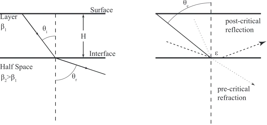
1.1 Refraction Nomenclature . . . 7
1.2 Relationship between shear wave velocity and apparent surface wave velocity . . . 8
1.3 Phase shift in a post critical wave . . . 10
1.4 Comparison of Coulombic and elastic models. . . 15
1.5 The Coulombic damping model and its hysteresis loop. . . 16
1.6 The elasto-plastic model and its hysteresis loop. . . 17
1.7 The Kelvin-Voigt model and its hysteresis loop. . . 20
1.8 Asymptotic behavior of a Kelvin-Voigt system . . . 22
1.9 Maxwell viscoelastic model. . . 23
1.10 The KVMB (Kelvin-Voigt-Maxwell-Biot) system . . . 24
1.11 Resonant Column Apparatus used by Ishimoto and Iida (1937). . . . 26
1.12 Resonant Column Apparatus (excerpted from ASTM-D-4015 (92)). . 29
1.13 Preferred borehole configuration for crosshole testing (excerpted from ASTM-D-4428(91)). . . 32
1.14 The seismic cone penetrometer test (SCPT). . . 34
1.15 Downhole test set-up and graphs . . . 35
1.16 Idealized soil-structure system . . . 39
1.17 Magnification factor versus frequency for an idealized viscoelastic sys-tem with a natural resonance frequency of 1Hz. . . 40
2.1 Forces acting on a horizontal soil element. . . 43
2.3 Coordinate system used in the derivation of shear and Love wave
equa-tions. . . 51
3.1 Nomenclature and layer properties for a single layer over a half-space 55 3.2 Nomenclature and layer properties for a layered system over a half-space 56 3.3 Coordinate system used in the polar coordinate derivation of the shear and Love wave equations. . . 67
3.4 Bessel function and an approximation using Equation (3.54). . . 71
3.5 Comparison between scaled Bessel function and cosine function . . . 72
3.6 The argument principle . . . 73
3.7 Finding roots using the argument principle . . . 75
4.1 Soil properties used to model a single elastic layer over a half-space. . 77
4.2 The motion stress vector versus depth . . . 78
4.3 Elastic mode evolution with increasing frequency . . . 80
4.4 Dispersion curves of the fundamental mode and first three overtones for a single elastic layer over a half-space (Figure 4.1). . . 81
4.5 Complex frequency plot for a purely elastic model . . . 83
4.6 Effect of viscosity on complex velocity . . . 84
4.7 The loss tangent is greater than unity when Ci > Cr. . . 86
4.8 Soil properties used to model a single viscoelastic layer over a half-space. 87 4.9 Viscoelastic mode evolution with increasing frequency (single layer over a half-space) . . . 88
4.10 Dispersion curves for a single viscoelastic layer over a half-space. . . . 89
over a half-space . . . 90 4.12 Loss tangent as a function of frequency for a single viscoelastic layer
over a half-space . . . 90 4.13 Ray path in a two layer system . . . 93 4.14 Soil properties used to model two elastic layers over a half-space. . . . 94 4.15 Mode evolution with frequency for two elastic layers over an elastic
half-space . . . 95 4.16 Motion-stress displacement component for two elastic layers over a
half-space . . . 96 4.17 Dispersion curves for two elastic layers over a half-space . . . 97 4.18 Soil properties used to model two viscoelastic layers over a half-space. 98 4.19 Viscoelastic mode evolution with frequency (Two layers over a
half-space). . . 99 4.20 Dispersion curves for two viscoelastic layers over a half-space . . . 100 4.21 Attenuation as a function of frequency for two viscoelastic layers over
a half-space . . . 100 4.22 Loss tangent as a function of frequency for two viscoelastic layers over
a half-space. . . 101 4.23 Soil properties used to model three viscoelastic layers over a half-space. 101 4.24 Love wave modes as a function of frequency for a three-layer elastic
system (Figure 4.23). . . 102 4.25 Dispersion curves for three elastic layers over a half-space . . . 103
tic system . . . 104
4.27 Dispersion curves for three viscoelastic layers over a half-space . . . . 105
4.28 Attenuation as a function of frequency for three viscoelastic layers over a half-space . . . 105
4.29 Loss tangent as a function of frequency for three viscoelastic layers over a half-space . . . 106
4.30 Higher order Love wave modes as a function of frequency for a three-layer viscoelastic system (Figure 4.23). . . 107
5.1 Source and receiver lay-out. . . 115
5.2 Gaussian white noise was added to the data from each trace. . . 123
5.3 Synthetic data shot gathers . . . 124
5.4 Masking a K-f plot before converting to frequency-space domain . . . 126
5.5 Comparison of K-f plots from low and high density lay-outs. . . 127
5.6 Constant wave numberslices obtained from Figure 5.5. . . 128
5.7 Expanded K-f plot of high density lay-out data. . . 129
5.8 Dispersion curves obtained from the low density lay-out. . . 130
5.9 Dispersion curves obtained from the high-density lay-out. . . 130
5.10 Attenuation curves from the low density lay-out. . . 131
5.11 Selected attenuation curves. . . 131
5.12 Attenuation curve obtained from fundamental mode. . . 132
5.13 Dispersion curves for synthetic two layer data. . . 133
5.14 Attenuation curves for two layer synthetic data. . . 133
5.15 Dispersion curves for three-layer synthetic data. . . 134
6.1 Convergence history for single mode data . . . 150 6.2 Convergence history for inversion of all four modes . . . 154 6.3 Convergence history for a two layer viscoelastic model. . . 157
A Motion Stress Coefficient Matrix.
C∗ complex Love wave velocity (ms).
Cr real Love wave velocity component (ms).
Ci imaginary Love wave velocity component (ms).
CL Love wave phase velocity component (ms).
D Damping factor for a viscous damping element (1
s2).
DR ASTM-D-4015 Damping Factor (Dimensionless).
DRc Damping factor used in the International Building Code (Dimensionless).
Gc Frictional force on a Coulombic damping element (N t).
Ge Spring coefficient (Hooke’s coefficient) (N tm).
Gv Viscous force on a viscous damping element (N tm).
h Equivalent single layer thickness (m.)
hj Layerj thickness (m).
i Imaginary Unit.
I1 and I2 Energy Integrals.
k∗ Complex shear angular wave number (radm).
K Real cyclical shear wave number (cycless ).
kr Real angular shear wave number (radm ).
ki Imaginary angular shear wave number/attenuation coefficient. (radm),(m1)
K∗ Complex Love angular wave number (radm).
Kr Real Love angular shear wave number (radm).
Ki Imaginary Love angular shear wave number/attenuation coefficient. (radm),(m1)
lmj Layer j motion-stress vector displacement component. lsj Layer j motion-stress vector stress component.
m,mˆ,∆m vector of model parameters, estimates, and differential values.
R(x) Horizontal wave equation eigenfunction in Cartesian coordinates (x) direction. L(z) Wave equation eigenfunction for the vertical (z) direction.
Q Eivenvecor matrix of A
sd, su Upward and downward propagation coefficients.
S(r) Horizontal wave equation eigenfunction in cylindrical coordinates (r) direction. T(t) Wave equation eigenfunction for time (t).
t Time.
u,v,w Displacement in, respectively, x, y, and z directions. U Group velocity (ms)
v(x,y,t) Horizontal (y) displacement function. x Ordinate in direction of wave propagation. y Transverse ordinate.
z Vertical ordinate, measured from the surface.
α p wave phase velocity (ms).
αL Love Wave Attenuation Ratio (radm ).
αs Shear Wave Attenuation Ratio (radm ).
β∗ complex shear wave velocity (ms).
βi imaginary shear wave velocity component (ms).
βr real shear wave velocity component (ms).
βs shear wave phase velocity (ms).
Error vector.
ε Phase delay (rad)
λj first Lam´e Parameter (P a), or spatial wave number (1/m).
Λ Eigenvalue matrix of A.
µj Layerj shear modulus (P a).
µ∗j Layerj complex shear modulus (P a).
ηj Layerj effective viscosity (P a−s).
ξs shear waveattenuation ratio.
ξL Love wave attenuation ratio.
ρj Layerj density (mkg3).
τj,k Stress component.
ω Angular frequency (rads ).
ωd Damped resonant angular frequency (rads ).
ω0 Undamped resonant angular frequency (rads ).
CHAPTER 1:
BACKGROUND AND HISTORICAL CONTEXT
Both the instrumentation and the theoretical apparatus for studying seismic waves evolved rapidly during the last two decades of the nineteenth century, and scien-tists were putting the devices to use exploring Earth’s deep structure. By the nine-teen twenties, it was widely recognized that Earth consisted of a solid inner core, surrounded by a liquid core, wrapped in a mantle, and covered with a thin outer crust. That the destructive power of earthquakes was primarily due to waves travel-ing through, and interacttravel-ing with, this thin crustal layer was also generally accepted (Fowler, 2005).
Cogent explanations for the visible manifestations of an earthquake’s destructive power were more problematic: A structure might be demolished, while a nearby structure might suffer little or no damage at all. By the late nineteen fifties, structural and geotechnical engineers had concluded that a structure’s behavior in an earthquake could best be understood in terms of a resonant system, consisting of the structure and ground to which that structure is attached. Modern building codes reflect this understanding by requiring that critical structures be designed to withstand lateral loads caused by the resonant behavior of the earth-structure system.
been made using cross-borehole experiments as described in ASTM-D-4428 (1996). This method allows in-situ testing to determine shear wave velocities, but because it requires three or more bore holes, it can be expensive (Michaels, 1998).
The advent of inexpensive horizontal-component geophones has made collection and inversion of shear wave data economically viable. In the present work, we will develop a novel method for estimating viscoelastic soil properties in-situ. Because Love wave velocity and attenuation are functions only of viscoelastic shear proper-ties, Love wave inversion avoids the pitfalls that might result when erroneous com-pressional properties are included in Rayleigh wave inversion schemes such as SASW and MASW.
1.1
Evolution of the Love Wave Analytical Model
Love waves result from interactions of horizontally polarized shear waves, within a zone of low velocity material, near Earth’s surface. Unlike Rayleigh waves, which arise from the interaction of vertically polarized shear waves with dilational waves at Earth’s surface, Love wave behavior depends solely on material shear properties.
Poisson (1830) derived general equations for wave propagation in elastic media, and demonstrated that within a homogeneous, isotropic solid body, there exist two distinct propagation modes. Dilational wave propagation is parallel to particle mo-tion, and its velocity is given by the relationshipα=
q
λ+2µ
ρ . Shear wave propagation is perpendicular to the direction of particle motion, and its velocity is given by the relationship β = qµρ. Thus, dilational wave propagation is necessarily faster than shear wave propagation, and by the mid-19th century, the monikers primary (P) and secondary (S) were being used describe the order in which these waves manifest themselves in seismic instrumentation (Stokes, 1849).
pattern: A weak preliminary tremor followed by a main shock. The causes of this pattern were the subject of scientific scrutiny through the first decades of the 20th century. Early on, it was believed that the preliminary tremor and main shock cor-responded, respectively, to P and S waves; however, this simple description was soon abandoned (Love, 1911). Although seismologists were in general agreement that the earliest signals corresponded with the arrival of P waves at Earth’s surface, neither the magnitudes nor the behavior of subsequent arrivals were consistent with S waves. A potential explanation was given by Lord Rayleigh. In 1885, Rayleigh predicted the existence of surface waves, and described a means by which they could be gen-erated through the interaction of P waves and vertically polarized S waves with the surface of an elastic body (Rayleigh, 1887). He demonstrated that these waves would travel somewhat more slowly than S-waves, and that unlike body waves, which decay directly with the distance from the source, Rayleigh’s eponymous waves decay with the square root of distance. Thus, at long distances, Rayleigh waves could be much stronger than body waves. Rayleigh also predicted that these waves would manifest themselves through elliptical particle motion at the surface, providing a theoretical underpinning for some of the late motions observed in seismograms.
Rayleigh’s theory was dependent on an earlier work by Lamb (1882), and Rayleigh himself noted that it was possible to derive his predictions using formulae derived in Lamb’s paper on elliptical waves in elastic spheres. In his discussion, Rayleigh disputed Lamb’s assertion that only positive real values of the bulk modulus and Poisson’s ratio yield stable solutions to his wave equations. Asserting that the only necessary conditions for stability are that shear modulus,µ, and bulk modulus,λ+2
3µ,
bulk modulus could be as small as zero, and that Poisson’s ratio could be as small as negative one.
Rayleigh discussed the mathematical possibility of complex solutions to the wave equations, but dismissed such solutions as lacking physical interpretation. In the present work, we will discuss a framework wherein complex solutions of wave equations not only have physical meaning, but utility, as well.
In 1900, Oldham published a system for seismic interpretation that associated events in the preliminary tremor with P and S body waves, and those in the main shock with Rayleigh waves (Oldham, 1900). Oldham’s interpretation of the prelimi-nary tremor was consistent with seismic data, and generally well received; however, the notion that the main shock consisted of Rayleigh waves was more controversial. Although velocities and magnitudes were consistent with those predicted for Rayleigh waves, other aspects of their behavior were not. For example, Rayleigh waves were predicted to operate in two dimensions, with the vertical component of motion larger than the horizontal component by a factor of between 1.5 and 2, yet the earlier por-tions of the main shock often exhibited little or no vertical motion. Furthermore, these early portions often exhibited substantial horizontal movement perpendicular to the direction of wave propagation (Love, 1911).
although he suggested that such periodicity could be explained by periodicity of the source, he was unable to explain the mechanism by which this might occur.
In 1911, A.E.H. Love published an essay entitled, Some Problems of Geodynamics, which won Cambridge University’s 1911 Adams prize. Love’s book tackles problems as diverse as isostacy, gravity anomalies, and ocean tides. In Chapter 11, after reviewing the theories of Rayleigh, Lamb, and Oldham, he proposed a mechanism to explain the lateral seismic motions that had vexed the Geosciences since the first accurate seismometers had become available.
Love proposed that a superficial layer of relatively slow material over a faster half space might act as a wave guide for horizontally polarized transverse waves (SH waves). Love demonstrated that such a system would be dispersive: Low frequency waves would travel more quickly than high frequency waves. Accordingly, the inter-action between Earth’s crust and the mantle could sort a relatively short burst of seismic energy, such as is produced by an earthquake, into a long train of periodic, large amplitude, lateral waves similar to those observed in the seismic record. In his essay, Love also developed a theory of Rayleigh wave propagation in layered me-dia, but he did not extend the method to the propagation of Love waves in layered media. In Chapter 3, our development of Love wave relationships will begin in a manner reminiscent of Love’s own work; however, our treatment will diverge so that we can extend it to layered media with viscoelastic properties. We will also derive relationships that will allow us to account for the effects of geometric spreading.
Layer
Half Space
Surface
β1
β2>β1
Interface
θi
θr
H
post-critical reflection
θc
pre-critical refraction ε
θi
θi
P R Q
Wave front
β1
C
Figure 1.2: Relationship between shear wave velocity and apparent surface wave velocity, C. The wave front is moving at an angle θi and velocity β1. In the time it
takes a point, P, on the wavefront to move to a point, R, on the surface, the surface expression of the wave front will have moved from pointQ to pointR. QR is greater than P R, so the apparent velocity, C, is greater than β1. Thus, surface wave phase
velocity, C, is greater than or equal to β1.
the interface from above to be reflected back into the layer. According to Snell’s law (Stein and Wysession, 2003), a shear wave traveling across the interface between a layer and a half-space will refract at an angle that depends on the incidence angle,
θi, and on β1 and β2. Beyond a certain critical angle, the wave will reflect back into
the original layer. The critical angle, θc, is found using Snell’s law:
sinθc=sin
π
2
β1
β2
= β1
β2
(1.1)
phase velocity equal to:
CL=
β1 sinθi
(1.2)
To an observer on Earth’s surface, a wave traveling upward and perpendicular to the surface, would appear to have an infinite velocity. If a wave’s incidence angle at the half-space boundary is less than θc, its energy will propagate into the half-space and be lost, and the wave will be unsustainable. This places an upper limit on the apparent velocity of Love wave propagation. Substituting Equation 1.1 into Equation 1.2, we see that maximum possible apparent Love wave velocity is β2, thus placing
upper and lower bounds on possible Love wave phase velocities: β1 < CL< β2.
Below the critical angle, a significant fraction of incident energy is transmitted downward into the half-space and lost. Although it is possible for the energy reflected back into the layer to interfere constructively and form leaky modes, these typically decay so quickly that they won’t be of concern to us in the present work. The inquisitive reader is referred to Section 7.6 of Aki and Richards (2009).
At post-critical angles, all of the energy incident upon the interface is reflected back into the layer; however, its phase is delayed by an angle, ε, that depends on the incidence angle and material properties of both layers. To understand the cause of this phase shift, recall that the apparent velocity of a post-critical wave on the layer side of the interface will be less than wave velocity in the half-space, β2. This
evanescent wave β1
Layer Half Space β2
Apparent wave velocity β1<C<β2
ε
Figure 1.3: Phase shift in a post-critical wave. The apparent phase velocity, C, of a post-critical wave impinging on the interface will be less than half-space velocity, β2,
and greater than layer velocity, β1. This mis-match causes a shallow stress field and
the reflected wave. Thus, a Love wave can properly be thought of as the product of constructive interference resulting from the interaction of a reflected wave with the evanescent wave.
The phase shift effect is also evident in the reflection coefficient of a post-critical wave, which is a complex number with a modulus of unity. The phase delay, ε, is the same for all frequencies; however, because wavelength is a function of frequency, the effect is to create a thicker evanescent wave in the half-space. In effect, longer wavelengths see a thicker layer than is seen by shorter wavelengths. This unequal treatment contributes to the dispersive behavior of Love waves: Love wave velocity,
CL, is frequency dependent, with the apparent surface velocities of low frequency waves greater than those of high frequency waves. The reader seeking a more rigorous treatment of evanescent waves and post-critical phase shift is referred to Section 2.6 of Stein and Wysession (2003).
Like a guitar string, a Love wave system can resonate at a fundamental mode and a number of overtones; however, the interpretation of each system’s fundamental mode and overtones is different. For a guitar string, the fundamental mode produces the single lowest frequency which can form a standing wave, and each overtone represents an integral multiple of the fundamental frequency. By contrast, an elastic layer over a half space can resonate at any frequency. As noted above, phase shift depends on incidence angle, so it is always possible to find at least one post-critical angle for which a given frequency can resonate. Of course, as noted in (1.2), each incidence angle is associated with a unique apparent velocity betweenβ1 andβ2, so a mode can be described by an infinite set of unique frequency-velocity pairs.
frequencies, from zero to infinity, with low frequencies propagating at velocities near the half-space velocity,β2, and high frequencies propagating at velocities closer to the
layer velocity, β1. Throughout this text, we will refer to the lowest mode (n = 0) as
the fundamental mode, and subsequent modes as the first overtone (n = 1), second overtone (n = 2), etc. Unlike the fundamental mode, the first overtone only exists at frequencies above a cut-off frequency, fcn. For an elastic layer over a half-space, the apparent velocity at fcn is equal to β2. The cut-off frequency is given by (adapted
from Stein and Wysession (2003)):
fcn =
nβ1
2h1 q
1−β21
β2 2
(1.3)
In Chapter 4, we will explore the dispersive relationships for each mode. Because these relationships are dependent on material properties, Love wave dispersion curves can provide information about layer properties. In Chapters 5 and 6, we will develop methods for determining layer structure and material properties using Love wave dispersion and attenuation curves.
the explosion. Thomson (1950) published a matrix formulation of the elastic surface wave problem that could be applied either to Love or Rayleigh waves. Haskell (1953) modified Thomson’s method and showed that it could generate Rayleigh wave disper-sion curves that compared favorably to those obtained from actual earthquake data. Although he derived a treatment for Love waves, he did not compare it to actual data. After developing a method for analyzing the dispersion curves obtained from Love waves, Takahashi (1955a) extended it to Rayleigh waves (Takahashi, 1955b).
The preceding models assume Earth materials to be purely elastic. Elastic Waves in Layered Media (Ewing et al., 1957), a popular text that focused primarily on determination of the layering structure of Earth’s crust, devoted a scant three pages to the Voigt model of internal friction; however, by the early 1960s, research on constitutive models incorporating friction was burgeoning.
1.2
Constitutive Soil and Rock Models
1.2.1
Coulombic Soil Damping Models
In 1773, Charles Augustin de Coulomb returned to Paris from a posting as a military engineer on the Island of Martinique. While on Martinique, Coulomb developed a theory of soil mechanics based on the theory of friction developed by Guillaume Amontons (1699). In short, Amontons’ three laws stated that frictional force was proportional to the applied normal force, that it was independent of contact area, and that frictional force is independent of sliding velocity. Coulomb’s work eventually earned him the sobriquet, Father of Soil Mechanics, but at the time, Amontons’ theories were controversial, so although Coulomb’s theory of soil mechanics was widely read (Coulomb, 1773), many believed its reliance on Amontons’ tribology to be a critical flaw. The theory of contact friction in soils began with controversy and, and as we will see, that is still the case more than two centuries later.
Not surprisingly, Coulomb’s next major work began with a lengthy section that used the results of his own detailed experiments to explain and defend Amontons’ theory (Coulomb, 1781). This paper won a major prize from the French Academy of Sciences, and Coulomb’s defense of Amonton’s theory was so successful, that the theory is now usually referred to as the Coulombic theory of friction.
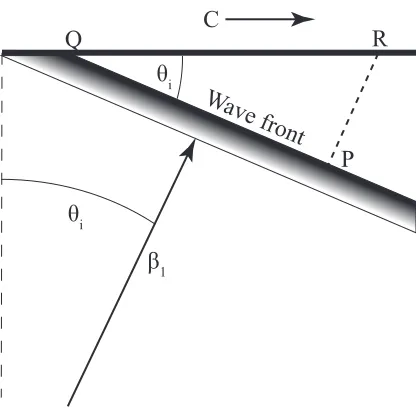
fm
um
1 2
4 3 Gc
fm
um
Figure 1.4: (l) After displacement, a purely Coulombic system (1) will not return to its original state. (r) After displacement, a purely elastic system returns to its original state along the path taken to its displaced configuration. Common elastic modeling elements include linear (2), bi-linear elastic (3), and non-linear (4) models.
never could completely reconcile it with his own observations.
It was Musschenbroek (1762) who pointed out that if friction were due to adhesion, then frictional forces would be a function of area. By Coulomb’s day, this criticism was taken very seriously. Noting that des Camus (1722) and Desaguliers (1719) had observed the frictional retardation of moving objects to be less than that of objects at rest, Coulomb developed the concepts of static and sliding friction. Under Coulomb’s model, static friction is due, primarily, to adhesion, and sliding friction is due to a different mechanism. Under this reformulation of Amontons’ third law, the coefficient of sliding friction is independent of sliding velocity.
fe = -Geu H(|F|-Gc)
fc= -Gcsgn(u) H(|F|-Gc)
m
um=ue= uc
F(t)
fm
um
1 2
3
4 5
Gc
-Gc 6
Figure 1.5: (l) Coulombic damping model. (r) When a unidirectional force, F(t), is applied to the system, it follows the force-displacement relationship indicated by paths 1 and 2. When F(t) is a periodic force, it follows hysteretic loop of paths 2, 3, 4, 5, and 6, and then repeats.
A purely elastic system tends to return to its original configuration without dissi-pating any energy. On a force-displacement plot, a purely elastic system follows the same path to and from its displaced configuration (figure 1.4r). Since a purely elastic system contains no mechanism for dissipating energy, once perturbed, it will vibrate indefinitely around its original configuration. No completely elastic systems exist in the macroscopic world: When struck, a bell may ring for a very long time, but it will eventually dissipate energy, and stop ringing (Lai et al., 1993).
There are two obvious ways to include an elastic term in a Coulombic friction model. In the Coulombic damping model, elastic and Coulombic elements are in parallel. In the elasto-plastic model, they are situated in series (Morrison, 2002).
fe = -Geue H(Gc-|Geue|)
fc= -Gcsgn(uc)H(Gc-|Geue|) m
fm= fe= fc
F(t)
fm
um
1 2
3 4
5 Gc
-Gc 6
Figure 1.6: (l) Elasto-plastic system: Elastic and Coulombic elements in series. (r) When a unidirectional force, F(t), is applied to the system, it follows the force-displacement relationship indicated by paths 1 and 2. WhenF(t) is a periodic force, it follows the hysteretic loop of paths 2, 3, 4, 5, and 6, and then repeats the cycle.
function H(|F(t)| −Gc). Once in motion, the frictional element exerts a constant force, Gc, opposite the direction of motion, and the elastic spring exerts a force that is equal to the relative displacement of the spring times the spring (Hooke’s) con-stant, Ge. A signum function, sgn( ˙u), ensures that the frictional term acts opposite the direction of motion (Figure 1.5). A physical analogue to this system might be a sponge, which, if deformed, will return to its original shape, albeit with a loss in the mechanical energy of the system.
If driven by an oscillating driving force, F(t), the force-displacement curve will assume the shape shown in Figure 1.5r. The area bounded by this curve is called a hysteresis loop, and it represents the energy lost by the system during each oscillatory cycle. When the maximum displacement amplitude isumax, the total hysteresis energy will just be the area inside the parallelogram (EH = 4umaxGc). If the driving force is removed, the system will oscillate, but its amplitude will decay with time.
displacement of each element will be different (Iwan, 1961). The spring deforms to a maximum displacement equal to ue = sgn( ˙uc)Gc/Ge before the Coulombic element begins sliding, and the force on the spring, mass, and Coulombic element will all equal Gc. If driven by an oscillating force, the force-displacement curve will assume the shape shown in Figure 1.6r. If the driving force is removed from a serially damped system, the system will oscillate and decay untilfm < Gc. After that point, decay will be zero for an ideal system. The elasto-plastic constitutive model is widely employed by geotechnical engineers (Desai and Christian, 1977).
An important characteristic of any frictional model is its dependence on loading. Under the original Amontons-Coulomb theory,Gcis a linear function of normal force. For soils, this translates into a dependency on effective stress, which, itself, is a function of depth, soil density, and pore water pressure (Das, 2011). Recall that elasto-plastic behavior remains elastic until the total force on the system exceedsGc: For a soil exhibiting elasto-plastic behavior, we expect depth to increase the force necessary to induce Coulombic behavior. On the other hand, once this threshold has been reached, and particles begin moving against each other, we would expect the effects of damping to be enhanced with depth. In practice, although we see a delayed onset of Coulombic behavior at depth, this is not as pronounced as Amontons-Coulomb theory, alone, would predict (Ishihara, 1996).
that can alter material properties (Morrison, 2002). Perhaps more importantly, a fundamental assumption of Amontons-Coulomb theory is that the contact surfaces be dry: In the real world, soil particles tend to be wet. Even in the vadose zone, most soil particles are coated with a thin water film (Fetter, 2001). Depending on film thickness, contact velocity, and contact surface geometry, this film can either act as a viscous lubricant, or as a hydrodynamic bearing surface (Burr, 1995).
Probably the largest obstacle to adoption of models with Coulombic elements is their computational difficulty. Mathematical models of Coulombic elements tend to be highly non-linear, and they are not generally amenable to closed-form analytical solution (Iwan, 1961). Even after the wide spread availability of digital comput-ers, calculations involving Coulombic elements remain computationally expensive. A common solution is to approximate Coulombic elements using visco-elastic elements.
1.2.2
Viscoelastic Models
fe = -Geu
fc= -Gvu m
um=ue= uc
F(t)
fm
um
1
Figure 1.7: (l) Kelvin-Voigt viscoelastic model. (r) When subject to an oscillating driving force,F(t), the force-displacement curve of a Kelvin-Voigt system describes a Lissajous curve.
damping and creep behavior that he observed in metal wires (Thomson, 1865). Thom-son’s viscoelastic model was a simple one-dimensional model similar to that shown in Figure 1.7. While working to explain the elastic behavior of crystalline solids, Voigt (1889) proposed a comprehensive viscoelastic model that is now generally referred to as either the Kelvin-Voigt model, or the Voigt model.
The Kelvin-Voigt (KV) model consists of an elastic element and a viscous element in parallel. The viscous term is characterized by the product of a viscosity factor, Gv and a velocity, ˙u, so that:
Fm =−Geu−Gv
du
dt =m
d2u
dt2 (1.4)
Rearranging Equation (1.4), and equating it in terms of a driving force, F(t):
d2u
dt2 +
Gv
m du
dt +
Ge
mu=F(t) (1.5)
equations, e.g. Asmar (2000). For an underdamped system (discussed in Chapter 2), the solution is:
u=e−Dt(C1cos(ωdt) +C2sin(ωdt)) (1.6)
where:
ωd=
r
G2
v 4m2 +ω
2
0 (1.7)
D= Gv
2m (1.8)
where D is a damping factor, ωd is the resonant frequency of the damped system, andω0 is the resonant frequency of the corresponding undamped system, i.e. Gv = 0. We will devote much of Chapter 2 to derivation of a viscoelastic soil model and wave equation analogous to Equation 1.6, but for now, we will consider some consequences of the Kelvin Voigt model of a lumped parameter system.
First, we note that the exponential term in (1.6) is a damping factor that depends on the ratio Gv/(2m). Second, we note that the resonant frequency of a damped system will always be higher than the resonant frequency of the corresponding un-damped system. This second, somewhat counterintuitive, result and its implications for wave propagation will be discussed extensively in the following chapters.
Geu
F/Ge
time
displac
emen
t--u m
for
ce
--f m
0 0
Figure 1.8: (l) When subject to a constant force, F, displacement of a Kelvin-Voigt system will approach, asymptotically, F/Ge. (r) When subject to a rapid displace-ment, the force on the mass will decrease, asymptotically, to zero. Materials Scientists refer to this behavior as creep.
1996), although competing models abound.
Much of the Kelvin-Voigt model’s appeal is its amenability to treatment by analyt-ical methods (Michaels, 1998), and it is possible to reformulate other models in terms of a Kelvin-Voigt model. For example, it is common practice to expres the Coulombic damping model in terms of a Kelvin-Voigt model that disperses the same hysteretic energy per cycle. As stated earlier, the total hysteretic energy lost by a single Coulom-bically damped cycle is Ec= 4Gcumax. The energy dissipated in a single viscoelastic cycle, found by integrating one cycle of the ellipse in 1.7, is Eve=πGvωu2max. Under an equivalent hysteretic energy formulation, we could impress the viscoelastic model into service as a Coulombic damping model by making the viscosity factor a function of frequency and displacement amplitude (Equation 1.9).
Gveq(ω, d) = 4Gc/(πωumax) (1.9)
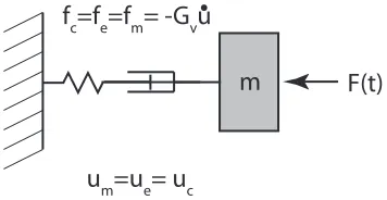
m F(t) fc=fe=fm= -Gvu
um=ue= uc
Figure 1.9: Maxwell viscoelastic model.
model (Stephens et al., 2000). We will discuss a variant of this technique that is in common use by practitioners reducing data from resonant column experiments. Arslan and Sihayi (2006) have outlined a generalized technique for incorporating non-linear behavior into KV constitutive models.
Of course, it is also possible to arrange the viscous and elastic elements in a series (Figure 1.9). This model was originally formulated by James Clerk Maxwell (1866) while developing a constitutive model for gas behavior, but it has gained widespread use as a rheological model for fluids and for solids that exhibit low-shear strain dependent behavior.
An interesting consequence of the Maxwell model is its prediction that at suffi-ciently high frequencies, fluids might be able to transmit shear waves. Indeed, Han et al. (2005) have demonstrated the ability of heavy, high viscosity oils to transmit shear waves at frequencies in the 100s of KHz toM Hz range.
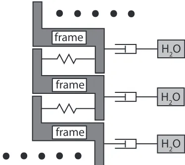
frame
frame
frame
H2O
H2O
H2O
Figure 1.10: Assemblage of Kelvin-Voigt-Maxwell-Biot (KVMB) systems (after Michaels (2006a))
flow is one of the few transient cases for which a closed-form analytical solution ex-ists. As envisioned by Biot, the fluid and frame act as coupled oscillating systems. An interesting consequence of Biot theory is the prediction that there exist two types of P-waves: One that exists primarily in the frame, but that is slowed somewhat by its interaction with the fluid, and another that exists primarily in the fluid, but that is sped-up somewhat by its interaction with the frame. Biot noted that at high frequencies, the assumptions of Poiseuille flow break-down, and published a second paper treating high frequency wave transmission (Biot, 1956b). Biot theory is ap-pealing because it is derived from fundamental mechanical principles. Unfortunately, as noted by Michaels (1998), implementation of Biot theory can be computationally cumbersome.
1.3
Testing Methods
We will briefly review two standardized methods for estimating viscoelastic soil pa-rameters: The resonant column test, which is described in ASTM-D-4015 (1996), Standard Test Methods for Modulus and Damping of Soils by the Resonant-Column Method, and the crosshole method, which is described in ASTM-D-4428 (1996), Stan-dard Test Methods for Crosshole Seismic Testing. We will also discuss in-situ tests that have been proposed as alternatives to these standardized methods.
1.3.1
The Resonant Column Test
response in his optical detector. In a collaboration, Ishimoto and Iida (1936) modified the device so that it could be used to determine the resonant frequency of soil samples and other unconsolidated media (Figure 1.11).
The resulting resonant column device consisted of an iron disk (base), on which was affixed a cellophane tube containing the soil sample (sample tube). Atop the soil sat another iron disk that compressed the soil sample into the tube (weight). The iron base was oscillated by means of an oscillating magnet. Iidra improved his resonant column device several times. Initially, oscillation of the weight was monitored mechanically, but in later versions, oscillation was monitored using a light and mirror. An advantage of the latter apparatus was that it could be used with moving photographic film to record transient signals. The device could also include an axial excitation mechanism and sensor, so that dilational properties could be measured, as well.
Iidra would vary the excitation frequency until he either obtained a maxima or a null point, calculate the dilational or shear wave velocity necessary for resonance, and then use the velocities so obtained to estimate Young’s modulus, shear modulus, Poisson’s ratio, and Lame’s parameters. By turning-off the instrument, and monitor-ing its transient response, he could calculate both normal and shear viscosity values. Iida’s last paper using a resonant column device, On the Elastic Properties of Soil, Particularly in relation to its Water Content, was published in September 1940 (Iida, 1940)
(Richart et al., 1970). Most instruments followed the general pattern set by Iidra; however, researchers often changed the methods for exciting the sample or measur-ing sample response. In most cases, the column was either excited or its response monitored using some sort of magnetic inductor. Such instruments are called free-free instruments, because both their base and weighted top are free (Figure 1.12). A second variant, with a fixed base and free top, was developed by Hall (Hall and Richart, 1963). In 1981, the American Society for the Testing of Materials adopted a standardized test using the free-free instrument, ASTM-D-4015 (1996). The method has been updated twice since that date.
In practice, a specimen is prepared, weighed, and its physical dimensions mea-sured. The resonant frequency is determined, and then machine power is cut-off. Vibrational decay is measured, and then the operator uses uses a series of calcula-tions, curves, or a Fortran program, to determine modulii and the damping ratio, defined as:
DR= ηω
2µ (1.10)
where η is soil viscosity, ω is angular frequency is radians per second, and µ is the shear modulus. Note that we have altered ASTM’s symbology to be consistent with that used throughout the rest of this paper.
Figure 1.12: Resonant Column Apparatus (excerpted from ASTM-D-4015 (92)).
on dry Ottawa sands, he concluded that soil viscosity varies inversely with frequency, such that ηω/G is a constant. This is, essentially, Equation (1.10). The 2 in the denominator of Equation (1.10) aligns the definition of damping ratio with that of a related quantity called the damping capacity. Hardin seems to have been surprised by this finding, and emphasized that this result was for dry sands only, and that this assumption probably only holds near the measurement frequency.
Rearranging Equation 1.10, we arrive at the surprising result that for a given soil sample, its viscosity is inversely proportional to the frequency at which the res-onant column test was conducted: η = 2G(DR)/ω. This very odd result, a material property that is dependent on test conditions, seems to belie a problem with the ASTM-D-4015 methodology.
Indeed, the requirement that the product of viscosity and frequency be constant is exactly what we would expect of a Coulombic damping model. In any event, it is diffi-cult to reconcile a constantηω/Gwith the static viscosity values that were published for the same materials in Hardin’s paper.
We should note that a resonant column instrument is a very crude device for determining frequency-material property relationships. For a given material, we are limited to the column’s resonant frequency and its overtones. Hardin indicated that he used the fundamental and first two overtones to arrive at his conclusion, but he didn’t actually publish any of the frequencies that he used; instead, he published normalized frequencies without giving the normalization factor. In another discussion, about confining pressure relationships, he gave a frequency ofω= 1290 rad/s, which is about 205 Hz. Given this frequency, his first and second overtones would have been about 610 Hz and 1025 Hz, respectively. In a discussion of one of Hardin’s earlier papers (Hardin and Richart, 1963), Rao (1964) asked whether, given Hardin’s caveat about the limited frequency range over which the constantηω/G assumption is valid, measurements taken at frequencies that are two or more orders of magnitude greater than what might be expected in an earthquake are really worthwhile.
much flatter for dry samples than for moist samples–This is consistent with the idea that a Coulombic model might be appropriate for dry soils.
Other criticisms have been leveled at the resonant column apparatus, itself. H.D. McNiven and C.B. Brown suggested that some of the resonant behavior being ob-served might be due to tube waves (McNiven and Brown, 1963). Viscosity measure-ments typically are made by switching off the power to the device; however, Wang et al. (2003) demonstrated that it could take several seconds for the magnetic field used by the inductor to collapse, and that during that time, the system would create a counter-emf that could explain some or all of the frequency-dependent viscosity effect. In other words, it is quite likely that the amplitude decay measurements used to determine damping ratio are at least partially due to the resonant column device, itself.
A final criticism could be leveled at nearly any laboratory test: It is difficult to know whether or not a laboratory sample is behaving as it would in-situ. Ishimoto and Iida (1936 and 1937), collected soil samples in a carefully designed sampling jar. After making a resonant column with a sample, they would disturb the same soil sample, and repack it into the same sampling jar. They determined that repacking the sample usually effected a 2x to 10x decrease in viscosity.
1.3.2
In-Situ Methods
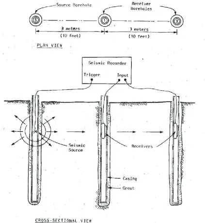
undisturbed. In practice, three boreholes are drilled along a line at 3mintervals, tak-ing care to disturb soils adjacent to each borehole as little as possible (Figure 1.13). Each hole is carefully cased and grouted. A seismic source is lowered into one of the outside holes, and receivers lowered into the two remaining holes so that all three are at the same height below the datum. The seismic source is triggered, and the signal recorded at each of the receivers. The process is repeated for several different heights using both p and s-wave sources. The data for each height and source is analyzed by using the difference in arrival times at the two receivers to determine the wave veloc-ity at each level. Using either assumed or measured soil densities, material properties such as shear modulus, Young’s modulus, and Poisson’s ratio can be determined.
Although not specified by ASTM-D-4428, it should be possible to determine at-tenuation coefficients provided that each receiver’s response characteristics are suffi-ciently well characterized.
The crosshole test’s main disadvantage is cost, and because the preferred spacing for the boreholes is relatively close (3m), multiple test locations might be necessary to survey an entire area of interest. ASTM-D-4428 provides a two hole method that can reduce costs somewhat; however, it would not generally be possible to extract attenuation information without at least three boreholes. Also, as was pointed out by Michaels (1998), the crosshole method is susceptible to the wave guide effect, which could cause elastic waves to experience dispersion, which would be easily confused for attenuation.
Figure 1.14: Seismic Cone Penetrometer Test (SCPT) developed by Robertson et al. (l) Cone penetrometer equipped with a rugged shear-wave seismometer. (c) Field test set-up. (r) Typical velocity-depth profile. Illustrations excerpted from Robertson et al. (1985).
Test (SCPT). The penetrometer is driven into the soil, and stopped at intervals so that its seismometer can be used to measure a signal generated by a horizontal shear wave source at the surface 1.14. The cone penetrometer test is less expensive than crosshole testing, and it has the advantage of producing correlative data that can be used to impute pore water pressure, median grain size (D50), relative density (Dr), unconsolidated shear strength (cu), overconsolidation ratio (OCR), drained friction angle (φ0), and bearing capacity factor (Nk) (Das, 2011). Although the authors did not do so, there would seem to be no impediment to using SCPT data to estimate damping coefficients. The main disadvantage of penetrometer tests is that the cone can have difficulty negotiating large cobbles or gravels.
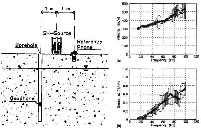
Figure 1.15: (l) Field set-up used by Michaels to obtain downhole data. (r) Typical dispersion (top) and attenuation (bottom) curves obtained from Michaels’ Idaho field tests. Illustrations excerpted from Michaels (1998).
there is no reason that this technique could not also be used with SCPT data. A receiver is lowered down a borehole and used to measure a signal generated by a horizontal shear wave source on the surface. The measured data is then inverted in a manner that best fits both the dispersion and attenuation curves obtained from the model (Michaels, 1998). These curves were obtained assuming a Kelvin-Voigt soil model.
The downhole method is a better choice for gravely soils than the SCPT method, and because it only uses one borehole, it is less costly than the crosshole method. It is also probably less susceptible to the effects of layering (wave-guide formation).
1.3.3
Surface Wave Methods
materials using Rayleigh waves. Although not central to his proposal, his development included a discussion of the Voigt viscoelastic model, with methods for correcting data for viscous attenuation. In 1981, J. Scott Heisey (1981), a graduate student at the University of Texas at Austin, wrote a Master’s thesis entitled, Determination of in situ shear wave velocities from spectral analysis of surface waves (Heisey, 1981). The next year, he and his collaborators published an extensive report of the same title for the Texas Department of Transportation, in which they detailed potential uses for the method (Heiseyet al., 1982). That same year, they published a paper entitled,Modulii of pavement systems from spectral analysis of surface wavesin ASCE’sTransportation Research Record. Kenneth Stokoe II, one of Heisey’s collaborators, has since published many papers on the Spectral Analysis of Surface Waves (SASW) technique.
advertised as a stand-alone method, SASW and MASW are probably best used in conjunction with techniques such as downhole, crosshole, or cone penetrometer tests. An important motivator for the use of shear wave techniques has been the Uni-form Building Code (ICBO, 1997) and its successor, the International Building Code (ICC, 2000). In order to estimate a structure’s earthquake response, both codes re-quire that the shear wave profile of the soils for any expensive or critical building project be determined to a depth of at least 30 m. Averaged shear velocity values then are used to impute earthquake site response and site amplification factors used for structural lateral load calculations. A 5% soil damping factor is used in base cal-culations; however, this may be adjusted depending on local soil conditions, or from the results of resonant column tests such as ASTM-D-4015 (1996). There currently is no requirement that damping ratio be imputed from in-situ tests; hence, there is little impetus to use SASW and MASW to estimate soil damping factors.
A second deterrent to using SASW/MASW to determine soil damping factors is the complexity of data inversion. Both methods use Rayleigh waves, which are de-pendent on dilational as well as shear properties. An inversion scheme using Rayleigh waves to determine shear properties would need to separate the effects of soil density, shear modulus, shear viscosity, bulk modulus, and bulk viscosity.
Most attempts at inverting surface wave data obtained from earthquakes have focused on purely elastic models. Pei (2007) has developed an interesting method that jointly inverts data from Love and Rayleigh waves to determine elastic parameters.
Jemberie (2002) modeled Rayleigh wave behavior using a Voigt-type model, and then used a least squares technique to determine the viscoelastic coefficients that best fit earthquake seismic data. Olsonet al.(2000) have used earthquake surface wave data to refine a viscoelastic model that used data from borehole logs as a control. Ho-Liu (1988) applied tomographic techniques to develop a viscoelastic model of crustal blocks in California’s Imperial valley; however, this study focused on the horizontal, rather than vertical structure of crustal blocks.
Chakravarthy (2008) has studied Love wave propagation in a single viscoelastic layer over a half-space. The difference between Love wave behavior of a single vis-coelastic layer and its purely elastic counterpart is striking. In Chapter 4, we will extend the study of a single viscoelastic layer to multiple viscoelastic layers.
1.4
The Need for Accurate Viscoelastic Soil
Property Estimates
The method prescribed by the International Building Code is a variant of the base shear force model: The structure is considered to be a stationary mass, under which, the soil and foundation oscillate with displacement, u, velocity ˙u, and acceleration ¨
Figure 1.16: (l) Idealized viscoelastic soil model with a sinusoidal wave traveling upwards to the surface. (r) Lumped parameterization of an idealized SDOF soil model.
Recall Equation 1.5. Setting F(t) =sin(ωt) we obtain:
d2u
dt2 +
Gv
m du
dt +
Ge
mu=sin(ωt) (1.11)
for which we define the magnification factor (MF) as the ratio of peak resonant amplitude to that of an untuned system. We will also define the critical damping ratio (DRc) for a lumped parameter SDOF system as the ratio of the damping coefficient to the damping coefficient that would effect critical damping. We note that definition differs from the ASTM definition used in resonant column testing (Equation 1.10). A complete derivation is found in the appendices of Kramer (1996):
M F = r 1
1− ω ω0
2
+
2DRcω
ω0
2 (1.12)
DR=0.5
DR=0.1
DR=0.05
DR=0
0.8 0.85 0.9 0.95 1 1.05 1.1 1.15 1.2
0 2 4 6 8 10 12
frequency (Hz)
Magnification Factor
Undamped Natural Frequency = 1 Hz
Figure 1.17: Magnification factor versus frequency for an idealized viscoelastic system with a natural resonance frequency of 1 Hz.
the magnification factor increases. Indeed, with no damping, it increases to infinity (Figure 1.17). Not surprisingly, magnification factor decreases rapidly with increasing damping ratio.
Idriss and Seed (1968) developed the SHAKE computer algorithm, which esti-mates surface displacement, velocity, and acceleration for layered soils over an os-cillating bedrock base. SHAKE has been immensely popular, and it has been the progenitor of several generations of software designed to estimate surface motion. As of this writing, SHAKE91 and SHAKE2000 are in common use. We should note that the various iterations of SHAKE use a bilinear hysteretic model–A variant of the Coulombic damping model. Nevertheless, the frequency dependence of magnification factors obtained using SHAKE are similar to those obtained using the viscoelastic model.
soils, as measured by resonant column tests, could be from one half to one tenth the value obtained from an undisturbed sample of the same soil. It is possible that a soil with a measured damping ratio of 0.5 could actually have a damping ratio of 0.05, so instead of a magnification factor near unity, the true, in-situ value might actually be closer to 10 (Figure 1.17). Even if it were possible to gather an undisturbed soil sample, that soil sample would represent just one point in the area of interest. Adjacent soils, or soils at different depths might be considerably different.
Crosshole and downhole tests avoid most of the pitfalls associated with laboratory testing; however, they are expensive. The seismic cone penetrometer test is less expen-sive, but can only be used with a limited range of soil types. Furthermore, crosshole, downhole, and seismic cone penetrometer tests only provide a velocity-depth pro-file for one point. MASW is a relatively inexpensive way to obtain vs30 information
over a fairly large area. Unfortunately, the complexity of Rayleigh waves has made determination of viscoelastic properties using either SASW or MASW problematic.
CHAPTER 2:
THE VISCOELASTIC SHEAR WAVE
EQUATION
In this chapter, we discuss our choice of the viscoelastic shear wave model, derive the viscoelastic wave equation, and then show how the viscoelastic wave equation can be transformed into a variant of the more common elastic wave equation. We will then solve the viscoelastic wave equation for a homogeneous half-space.