Elite Accumulative Sampling Strategies
for Noisy Multi-Objective Optimisation
Jonathan E. Fieldsend Computer Science, University of Exeter, Exeter, UK
Abstract. When designing evolutionary algorithms one of the key
con-cerns is the balance between expending function evaluations on explo-ration versus exploitation. When the optimisation problem experiences observational noise, there is also a trade-off with respect to accuracy refinement – as improving the estimate of a design’s performance typi-cally is at the cost of additional function reevaluations. Empiritypi-cally the most effective resampling approach developed so far is accumulative re-sampling of the elite set. In this approach elite members are regularly reevaluated, meaning they progressively accumulate reevaluations over time. This results in their approximated objective values having greater fidelity, meaning non-dominated solutions are more likely to be correctly identified. Here we examine four different approaches to accumulative resampling of elite members, embedded within a differential evolution algorithm. Comparing results on 40 variants of the unconstrained IEEE CEC’09 multi-objective test problems, we find that at low noise levels a low fixed resample rate is usually sufficient, however for larger noise magnitudes progressively raising the number of minimum resamples of elite members based on detecting estimated front oscillation tends to improve performance.
Keywords: Pareto optimality, differential evolution, uncertainty, noise.
1
Introduction
Many real-world optimisation problems experience noise which corrupts the ob-served quality values associated with a design. This may be due to, e.g., sen-sor/measurement error or environmental variation during the evaluation of a built design in embodied optimisation, or due to the stochastic nature of the software simulation being optimised (repeated evaluations leading to slightly different criterion values). Early multi-objective optimisation work raised the issue of noise affecting an evolutionary optimiser [15], but practical work devel-oping evolutionary multi-objective algorithms in this area did not commence in ernest until nearly a decade later. There now exist a wide range of ‘noise-tolerant’ algorithms, designed specifically for multi-objective optimisation problems with observational noise, e.g. [16, 17, 2, 27, 5, 3, 4, 8, 18, 1, 30, 12, 9, 6, 13, 24, 26, 20, 23,
10], and recent work has explored the situation where the objective functions themselves are inherently uncertain [29].
The vast majority of noise-tolerant optimisers include some form of resam-pling (repeated function reevaluation) of designs, in order to improve the esti-mate of their associated objective values. This is required as noise will mean that poor solutions with ‘favourable’ noise will be seen as better than they should be, and likewise good solutions that experience detrimental noise will be seen as relatively worse. This has the effect of corrupting fitness assignment and rank-ing, polluting any elite sets that may be maintained, and generally degrading optimiser performance. Furthermore, it has been observed in a number of studies that as the estimated non-dominated set converges the main driver for updating this set tends to be noise rather than improvements in the designs themselves (see e.g. [12, 13, 10]). This can seriously impede the ability of an algorithm to locate the Pareto front within the tolerance of the noise width(s).
There are many different approaches taken to resampling in the field, from static approaches, where a fixed number of resamples are taken for each design assessed, through to dynamic approaches based on, for example, reducing the standard error to within an acceptable bound. The reader is directed toward recent work by Siegmundet al. [25] for a full categorisation.
In the work presented here we are solely concerned withaccumulative sam-pling approaches (see e.g. [20, 10]). These require only a maximum likelihood estimator function being available, est(·), which takes a set of reevaluated ob-jective vectors associated with a design and provides the best estimate of the underlying noise-free objectives. This differs from a large number of other sam-pling approaches which rely on the noise experienced being Gaussian, and often utilise variance and standard error estimates [17, 2, 8, 26, 23, 25].
Accumulative sampling approaches leverage the observation that increasing the number of samples will increase the fidelity of the derived objective vector estimate irrespective of the noise density experienced, as long as the estimator is unbiased. That is, at the limit of infinite resamples the estimator will return the noise-free objective vector. Furthermore, even in the case where an estima-tor converges to the noise-free objective vecestima-tor plus a bias, dominance-based optimisation can still be performed effectively, as adding a constant does not affect the relative Pareto ranking of solutions [10]. In accumulative resampling of elite members, where the number of reevaluations per member is not limited, there needs to be decision regarding how many function evaluations should be expended on reevaluating elite members. In [20] the elite set is fixed in size, and each generation the entire elite set is resampled once, with a correspond-ing number of brand new designs also evaluated. In [10] each iteration of the algorithm results in a single new design, and the elite member with the fewest reevaluations is reevaluated a single additional time, with the last 5% of a run entirely devoted to reevaluations. As such, both [20] and [10] split their allocated function evaluations roughly equally between new proposals and previously eval-uated proposals. Experiments at the end of [10] however indicate that an equal balance between reevaluations and new design evaluations is not optimal for all
problems. Here we examine the use of adaptive reevaluation approaches for elite member accumulative resampling, including methods that ensure the number of effective reevaluations per member increases over time along with methods to increase the reevaluation rate if convergence is impeded by noise.
The rest of the paper is structured as follows. In Sec. 2 the multi-objective optimisation problem with observational noise is defined, along with basic re-sampling definitions. In Sec. 3 the properties of elite accumulative rere-sampling are discussed, and the proposed adaptive methods described. In Sec. 4 the dif-ferent approaches are compared empirically on the unconstrained problems of the IEEE CEC’09 multi-objective test suite, modified with additive noise with a range of magnitudes. Sec. 5 contains the paper conclusion and discussion.
2
Multi-objective optimisation with noise
Without loss of generality the multi-objective optimisation problem seeks to simultaneously minimise D objectives: fd(x), d = 1, . . . , D where each ob-jective depends upon a vector x = (x1, . . . , xp, . . . , xP) of P parameters or decision variables. The parameters may also be subject to equality and in-equality constraints which, for simplicity, we assume can be evaluated precisely. The multi-objective optimisation problem may thus be expressed as: minimise
f(x) = (f1(x), . . . , fD(x)), subject to the constraints which define X ∈RP, the
feasible search space. When there are multiple competing objectives, solutions may exist for which performance on one objective cannot be improved without degrading performance on at least one other. Such solutions are said to bePareto optimal. The set of all Pareto optimal solutions is said to form thePareto set, whose image in objective space is known as thePareto front.
A decision vectorxis said todominate anotherx0 ifffd(x)≤fd(x0) ∀d= 1, . . . , D and f(x) 6= f(x0). This is often denoted as x ≺ x0. Pareto domi-nance is a key comparator used in a wide range of evolutionary optimisers – either directly in their fitness assignment and ranking schemes, or as a means to identify their final Pareto set estimate. Elitist multi-objective optimisers gen-erally maintain a mutually non-dominating set A (often called an archive) of solutions which form their estimated Pareto set at any stage in their optimi-sation. This may be active (providing input into the optimisation process) or a passive record of the best solutions ever encountered during the optimisation [28]. In a noisy optimisation problem we cannot directly accessf(x), instead we have access to y, which are the criteria contaminated by observational noise . Here we are concerned with additive noise:
yd=fd(x) +d. (1) With n repeated reevaluations at a design locationx we obtain a set of noise contaminated objective vectorsY(x) ={yi}ni=1, which, in conjunction with an
unbiased maximum likelihood estimator will provide us with an estimate of the noise-free evaluation of f(x): fd(x) = est(Y(x)). For instance, if the noise was
Gaussian then est(·) would be the mean function, whereas if the noise was Laplacian it would be the median function.
In the noisy situation, we no longer have certainty that one solution domi-nates another (or that they are mutually non-dominating), as theexperienced by each solution may be of a value sufficient to reverse the ordering of solutions on one or more objective criteria. However, as n increases, our approximation to f(x) improves (in general this accuracy improves proportionally to √n). In order to ensure the exploitation of elite members uses accurately labelled de-signs, recent noise-tolerant optimisers have focused on resampling elite members preferentially [20, 10].
3
Adaptive accumulative sampling
Depending on the problem and the noise experienced, the update dynamics of the elite set may vary considerably. If members are regularly leaving the elite set, and new members regularly entering it, then the number of reevaluations per elite member may be in effect quite low – even when reevaluating an elite member for each new solution evaluated. Alternatively, if the membership of A
changes relatively irregularly, then the n per elite member may be very large. Neither of these situations may be ideal in practice, as in the first instance the elite members may fail to accumulate sufficient resamples to mitigate the noise when in proximity to the Pareto front, and in the second case some of these function evaluations may be better expended on new designs.
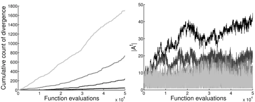
One side-effect of reevaluating previously evaluated solutions is that the esti-mated Pareto front canoscillate. This is distinct from the oscillating/retreating front issue derived from truncating elite sets in noiseless problems [14, 11], as its root cause is due to the (estimated) objective location of previously elite solutions moving, rather than the direct exclusion of solutions that are known with certainty to be non-dominated. This therefore affects even unbounded elite sets in the noisy case. An illustrative example is provided in Fig. 1. Here the differential evolution for multi-objective optimisation (DEMO) algorithm [21] is applied to noisy variants of the IEEE CEC’09 UP1 problem, with varying levels of additive observational Gaussian noise. The population in DEMO is main-tained using non-dominated sorting, so, subject to the population limit being sufficient to contain the number of non-dominated solutions encountered at any time point, on first glance the populationshould contain the best performing so-lutions found so far (as it will only discard dominated soso-lutions). However, this maintenance approach is not sufficient in the noisy case with reevaluations – as solutions may be discarded which would later be determined as non-dominated due to reevaluations of elite members degrading their estimated performance (‘exposing’ the previously dominated solutions). In Fig. 1 we expend one elite member reevaluation for every new design evaluated. The left panel of Fig. 1 shows the number of times the non-dominated subset of the DEMO search pop-ulation did not contain the non-dominated subset of all designs visited so far (based on theirest(·)). A secondary elite archive is maintained separately from
0 1 2 3 4 5 x 10⁴ 0 200 400 600 800 1000 1200 1400 1600 1800 Function evaluations
Cumulative count of divergence
0 1 2 3 4 5 x 10⁴ 0 10 20 30 40 50 Function evaluations |A t |
Fig. 1.Empirical oscillation of estimated elite members with Gaussian observational
noise on the UP1 problem. Noise standard deviations σ = {0.01,0.1,1.0,10.0} used for four different runs of the DEMO algorithm using elite reevaluations.Left: cumula-tive number of times the search population in DEMO needed to be updated using a secondary tracking archive (black through to light grey indicates low noise through to high noise).Right: Corresponding archive size,|At|. Note that|At|never exceeds 100
– the size of the non-dominated sorting truncated search algorithm in DEMO – but the search population regularly discards solutions which later become non-dominated (and have to be fed back in again) due to the reevaluation of the noisy solutions.
the DEMO population, using the techniques described in [7], and is merged in with the search population whenever they are detected to have diverged (redi-recting the DEMO population back to the estimated optimal regions of design space). This recalibration can be seen to be regularly required even when the search population membership is much larger than that of the elite set (an order of magnitude bigger in the highest noise case).
We now propose a number ofadaptive schemes for incremental accumulative sampling, and discuss the reasoning behind them. Each approach treats the op-timisation as an incremental process. At each time stept either a new design is evaluated, or a previously evaluated elite solution is reevaluated. In both situa-tions the membership of At (the estimated elite set at timet) may be altered, as in the first instance the new design may enterAt, and in the second instance reevaluation may cause the previously elite member to be dominated and/or move to a position in objective space such that solutions that were previously identified as dominated should now (re)enter the elite set.
3.1 Fixed resamples per generation
The baseline approach evaluates one new design per algorithm iteration, and reevaluates a single member of the elite set. The reevaluated elite member is that with the fewest reevaluations contributing to its estimated objective values.1
1
Selection could instead be based on the largest standard error for situations where
Algorithm 1Resample rate fixed over time.
Require: At−1 Elite non-dominated members identified at previous time step
Require: Xt−1 Other previously evaluated designs (dominated att−1)
1: At:=At−1,Xt:=Xt−1
2: Propose and evaluate new design, updateAt andXt
3: Reevaluate the member ofAt with fewest resamples, updateAt+1andXt+1
The evaluation of a new design may cause a change in the elite set or a change in the set containing all previously evaluated dominated solutions at a time step (Xt). The reevaluation of a solution may also cause multiple changes in both sets, as it can mean the removal of elements from Atto insert into Xt(if the reevaluated solution has moved to a dominated locations, or to a location that now dominates members of At), and the addition of elements from Xt toAt(where designs that were previous dominated are now categorised as non-dominated due to the reevaluated solution moving to an objective space location which no longer covers them). A basic outline is presented in Alg. 1.
3.2 Increasing resample rate, based on detecting false convergence
As mentioned above, one of the key issues with noisy optimisation problems is that as an algorithm converges, there is a tendency for noise to drive the search process over improving performance on the underlying criteria. One way of detecting this is to compare the state of the best elite set estimate at one time step,At, with that of an earlier time step, e.g.At−m. If the performance ifAt isworse than that ofAt−mthen (assumingAhas not been truncated) this can only be because reevaluations of members of Ain themintervening time steps has meant that their predicted locations throughest(·) have worsened, and that this shiftbackwards ofAthas not been compensated for by finding other designs which provide equivalent or better predicted performance to those inAt−m. In other words, the noise experienced made At−m seem better than it was, and we have not found any solutions (or reevaluated any) in the interveningmtime steps to compensate for this over-estimate. In order to mitigate this, the number of reevaluations areincreased, making it harder for rogue reevaluations to unduly influence the performance assessment (as outliers should be more quickly diluted with subsequent reevaluations).
Alg. 2 outlines this approach using the binary+ indicator (other indicators could also be used, see [19] for a discussion of different indicators and their properties). If the additiverequired to make theAt−mset dominate theAtset is lower that the value required to make theAtset dominate theAt−mset then the number of reevaluations per iteration is increased. Here the objective values are normalised by the bounds of the minimum bounding box containingAtand
At−m, and theest(·) used are those calculated for the designs at the respective time steps. Rather than compare Atwith At−mat every time step this is done everymtime steps as a minimum (lines 3-7). This allows the increment ofk(the
Algorithm 2Increasing resample rate based on convergence assessment.
Require: k Current resample number
Require: m Convergence time window
Require: At−m Elite non-dominated members identified at time stept−m
Require: At−1 Elite non-dominated members identified at previous time step
Require: Xt−1 Other previously evaluated designs (dominated att−1)
1: At:=At−1,Xt:=Xt−1
2: Propose and evaluate new design, updateAt andXt
3: if number of time steps since last check meets or exceedsmthen
4: if I+(At, At−m)> I+(At−m, At)then
5: k:=k+ 1
6: end if
7: end if
8: fori= 1, . . . , kdo
9: Reevaluate the member ofAt+i−1with fewest resamples, updateAt+iandXt+i
10: end for
number of reevaluations per iteration) time to have an effect before the sets are compared once more.
3.3 Increasing minimum revaluation number, based on detecting
false convergence
An alternative approach to increasing the absolute number of reevaluations each iteration, is to increase the minimum number of reevaluations that archive mem-bers must have accrued. This approach means the balance of function evaluations expended on reevaluations versus new designs can alter back and forth from one iteration to the next. For instance, if the minimum number of reevaluations per elite member was k = 10, after reevaluating a single archive member with the fewest reevaluations (Alg. 3 line 8), if all elite members had at least k reeval-uations then no further reevalreeval-uations would be taken. On the other hand, if there were elite members with fewer thankreevaluations, then the loop on lines 10-13 may be processed many times before the minimum number of reevalu-ations condition was satisfied. Note that the check to increase k (lines 3-7) is only undertaken in situations where the elite archive meets the condition that all members have at leastkreevaluations each.
3.4 Increasing average resamples per elite member
As the optimiser progresses we would like to say that the confidence we have in our elite set (our estimate of the Pareto set) increases rather than decreases or stagnates. With accumulative sampling the way to achieve this is to ensure that the number of reevaluations per set member is always increasing. Comparing one generation directly to the next can be a brittle approach as it may force a relatively large increase in resamples each time step (for instance if |A| = 1 for any stretch of time the imposition of an extra reevaluation each iteration
Algorithm 3 Increasing minimum number of reevaluations for elite members, based on convergence assessment.
Require: m Convergence time window
Require: At−m Elite non-dominated members identified at time stept−m
Require: At−1 Elite non-dominated members identified at previous time step
Require: Xt−1 Other previously evaluated designs (dominated att−1)
1: At:=At−1,Xt:=Xt−1
2: Propose and evaluate new design, updateAt andXt
3: if number of time steps since last check meets or exceedsmthen
4: if I+(At, At−m)> I+(At−m, At)then
5: k:=k+ 1
6: end if
7: end if
8: Reevaluate the member ofAt with fewest resamples, updateAt+1andXt+1
9: i:= 1
10: whilemember ofAt+iwith fewest resamples has fewer thankreevaluationsdo
11: Reeval. the member ofAt+i with fewest resamples, updateAt+i+1 andXt+i+1
12: i:=i+ 1
13: end while
Algorithm 4Increasing resamples per elite member over time.
Require: At−1 Elite non-dominated members identified at previous time step
Require: Xt−1 Other previously evaluated designs (dominated att−1)
Require: α Average number of resamples ofAacross all previous time steps
1: At:=At−1,Xt:=Xt−1
2: Propose and evaluate new design, determineAt andXt
3: Reevaluate the member ofAt with fewest resamples, updateAtandXt
4: i:= 1
5: whilemean num resamp(At)≤αdo
6: Reevaluate member ofAt+i−1 with fewest resamples, updateAt+iandXt+i
7: i:=i+ 1
8: end while
can be putative if the set grows in size later during an optimisation). Instead we examine a less stringent average approach here, as outlined in Alg. 4. Here the average number of resamples of solutions in Atis compared to the average across elite members of all previous time steps, and repeated reevaluations are taken if the current average is lower (lines 4-6). This is in addition to the extra reevaluation taken each generation as standard (line 3), which acts to steadily increase the lower bound on this minimum.
4
Empirical results
We now compare Algs. 1-4 empirically. We use the DEMO algorithm [21] to gen-erate a new design at each iteration prior to elite set member reevaluation(s). We modify the original DEMO in two ways to use in the noisy optimisation
con-Algorithm 5Incremental differential evolution candidate creation,p.
Require: Zt−1 DEMO population at previous time step
1: p:=copy random member(Zt−1)
2: {a,b,c}:=copy random members(Zt−1\ {p})
3: fori:= 1, . . . ,|p|do
4: if rand()<cross probthen
5: pi:=ai+differential weight×(bi−ci)
6: end if
7: end for
text. Firstly, in order to make the algorithm incremental a single new candidate design is generated from the DEMO population at each time step rather than doubling the population size (before its reduction via ranking and crowding). This is achieved at each algorithm iteration by selecting one of the DEMO pop-ulation at random to be the base parent (see Alg. 5, line 1). Secondly, due to the noisy environment, there is no guarantee that non-dominated solutions preserved by ranking and crowding truncation at one time step in the DEMO population will be non-dominated on reevaluation (as illustrated in Sec. 3). To mitigate this, a separate elite setAtis maintained using the data structures introduced in [7],2
and whenever the DEMO search population,Zt, does not containAt, the omit-ted members are combined withZtprior to DEMO’s truncation operator being applied. This was found to significantly improve the performance of DEMO in the noisy domain in our preliminary experimentation.
Further details describing DEMO may be found in the original work [21]. We use a DEMO population of 100 in all experiments, a probability of crossover of 0.9 and differential weight of 0.5. The external archive|At|is unbounded, and is updated at each time step using the data structure from [7] to ensure it contains the best estimate of the Pareto set. The algorithm variants are evaluated on the IEEE CEC’09 test suite3 [31]. We use the unconstrained (bounded)
prob-lems from the suite, UP1-10, with the standard number of design parameters, and modify the objective values with independent additive Gaussian noise with standard deviations ofσ={0.01,0.1,1.0,10.0}(making 40 test problem variants in total). In (1) therefore d∼ N(0, σ2). We run each algorithm 30 times, for a total of 300,000 function evaluations, and record the generational distance (GD) and inverse generational distance (IGD) every 500 function evaluations using the At at that time point. The noise-free reevaluation of the storedAt is used – the corresponding non-dominated set in its mapping to the noise-free space is extracted for the calculation of the quality measures. We utilise the modified versions of the GD and IGD quality measures which are not susceptible to vari-ation in set size (see [22]). We set the convergence check parameterm= 100 for all experiments.
2
Matlabcode fromhttps://github.com/fieldsend/.
3
Matlab code from http://web.mysites.ntu.edu.sg/epnsugan/PublicSite/ Shared Documents/Forms/AllItems.aspx.
0.010.1 1 10 0 0.1 0.2 0.3 0.4 0.5 0.6 0.7 0.8 0.9 1 Alg. 1 σ
Prop. across ranks
0.010.1 1 10 Alg. 2 σ 0.010.1 1 10 Alg. 3 σ 0.010.1 1 10 Alg. 4 σ 0.010.1 1 10 0 0.1 0.2 0.3 0.4 0.5 0.6 0.7 0.8 0.9 1 Alg. 1 σ Sig. better 0.010.1 1 10 Alg. 2 σ 0.010.1 1 10 Alg. 3 σ 0.010.1 1 10 Alg. 4 σ
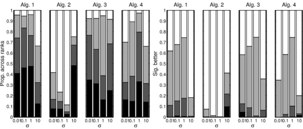
Fig. 2.IGD results, initial 10% of run. The left block of bar charts shows the proportion of time, across problems and polled every 500 function evaluations, where a resampling technique led to the best results (black), the second best (dark grey), third best (light grey) and worst (white), for each noise level. The right set of bar charts shows the corre-spondingsignificance assessments – black indicates the proportion where the approach is significantly better than all three other sampling approaches, dark grey significantly better than two, light grey significantly better than one and white not significantly better than any others.
0.010.1 1 10 0 0.1 0.2 0.3 0.4 0.5 0.6 0.7 0.8 0.9 1 Alg. 1 σ
Prop. across ranks
0.010.1 1 10 Alg. 2 σ 0.010.1 1 10 Alg. 3 σ 0.010.1 1 10 Alg. 4 σ 0.010.1 1 10 0 0.1 0.2 0.3 0.4 0.5 0.6 0.7 0.8 0.9 1 Alg. 1 σ Sig. better 0.010.1 1 10 Alg. 2 σ 0.010.1 1 10 Alg. 3 σ 0.010.1 1 10 Alg. 4 σ
Fig. 3.GD results, initial 10% of run. Description as in Fig. 2 caption.
Figs. 2 and 3 give the relative IGD and GD performance for the four reeval-uation routines embedded in DEMO, at each of the noise levels, averaged across the first 10% of the runs over the 10 test problems.4For low noise levels the single
revaluation approach has generally good performance for both quality measures, ranking first or second roughly 80% of the time across the initial stages of the
4
5% statistical significance is assessed using paired Wilcoxon signed ranks tests, with each strategy compared to each of the other competitors.
0.010.1 1 10 0 0.1 0.2 0.3 0.4 0.5 0.6 0.7 0.8 0.9 1 Alg. 1 σ
Prop. across ranks
0.010.1 1 10 Alg. 2 σ 0.010.1 1 10 Alg. 3 σ 0.010.1 1 10 Alg. 4 σ 0.010.1 1 10 0 0.1 0.2 0.3 0.4 0.5 0.6 0.7 0.8 0.9 1 Alg. 1 σ Sig. better 0.010.1 1 10 Alg. 2 σ 0.010.1 1 10 Alg. 3 σ 0.010.1 1 10 Alg. 4 σ
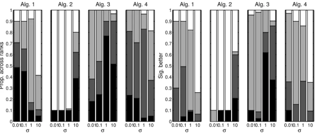
Fig. 4.IGD results, final 10% of run. Description as in Fig. 2 caption.
0.010.1 1 10 0 0.1 0.2 0.3 0.4 0.5 0.6 0.7 0.8 0.9 1 Alg. 1 σ
Prop. across ranks
0.010.1 1 10 Alg. 2 σ 0.010.1 1 10 Alg. 3 σ 0.010.1 1 10 Alg. 4 σ 0.010.1 1 10 0 0.1 0.2 0.3 0.4 0.5 0.6 0.7 0.8 0.9 1 Alg. 1 σ Sig. better 0.010.1 1 10 Alg. 2 σ 0.010.1 1 10 Alg. 3 σ 0.010.1 1 10 Alg. 4 σ
Fig. 5.GD results, final 10% of run. Description as in Fig. 2 caption.
optimisation. This is seen to drop off as the noise increases. The minimum elite member reevaluation approach (Alg. 3) performs fairly consistently across the noise levels, and performs better than the steadily increasing reevaluations ap-proach. Interestingly the approach which increases the number of reevaluations at each iteration (if oscillation is detected) tends to perform worst, except for the largest noise level, where its relative performance jumps up.
Figs. 4 and 5 provide the combined results for the final 10% of the runs. The general trends are as for the first 10% but the relative decline (and rise) of the reevaluation approaches as the noise level increases is more pronounced. The single revaluation approach degrades more steeply as the noise level rises, such that betweenσ= 0.1 andσ= 1.0 the minimum elite member reevaluation approach (Alg. 3) replaces it as being the preferred approach. Indeed, this ap-proach is best or second best for IGD 90% of the time for the highest two noise values.
Alg. 1 Alg. 2 Alg. 3 Alg. 4 0 1 2 3 4 5 x 10⁴ 0 20 40 60 80 100 Function evaluations
Av. reevals per elite member 0 1 2 3 4 5
x 104 0 500 1000 1500 2000 2500 Function evaluations
Av. reevals per elite member 0 1 2 3 4 5
x 104 0 50 100 150 200 250 300 Function evaluations
Av. reevals per elite member 0 1 2 3 4 5
x 104 0 20 40 60 80 100 Function evaluations
Av. reevals per elite member
0 1 2 3 4 5 x 10⁴ 0 10 20 30 40 50 Function evaluations |A t| 0 1 2 3 4 5 x 10⁴ 0 10 20 30 40 50 Function evaluations |A t| 0 1 2 3 4 5 x 10⁴ 0 10 20 30 40 50 Function evaluations |A t| 0 1 2 3 4 5 x 10⁴ 0 10 20 30 40 50 Function evaluations |A t|
Fig. 6.Average number of resamples per elite member elite on a single run on UP1
(top) and size ofAt (bottom) for each update algorithm. Black through to light grey
indicates low noise through to high noiseσ= 0.01,0.1,1.0,10.0.
4.1 Population dynamics
We can explore some of the different behaviours of the resampling regimes by examining the elite population dynamics over time, which also lends insight as towhy particular approaches seem better suited to different noise regimes. Fig. 6 shows the average number of reevaluations per member of At as a run pro-gresses through to 50,000 function evaluations on the UP1 problem for each of the accumulative sampling schemes, for the four different noise magnitudes. Some immediate differences become apparent. When noise is high the standard ap-proach of fixing the ratio of resamples to new design evaluations throughout the run can lead to fronts with large oscillations in the average number of resamples per member (repeatedly jumping across the range of 2-15 in a few iterations). On the other hand, increasing the number of reevaluations progressively each time the front is detected as oscillating (Alg. 2) leads to rapidly increasing aver-age number of reevaluations, meaning a relatively small proportion of expended evaluations are on new designs. Alg. 3 (setting a minimum number of resam-ples for archive members, and increasing this if convergence issues are detected) can be seen to balance these properties, with the average number of resamples increasing steadily in all noise regimes, but not drastically, and the variation rel-atively small from one iteration to the next. Correspondingly, although the size of Atvaries over time, it is seen to have lower amplitude on its high frequency oscillations (indicating lower churn of elite members with this approach). Alg. 4 similarly removes the wild variation in the average number of reevaluations experienced by members of Atwhich Alg. 1 and Alg. 2 are susceptible to, how-ever as the noise level increases the lower bound on this can be seen to plateau, rather than steadily increase as in Alg. 3. This decay is due Alg. 4 comparing the current average reevaluations per member of At with all previous archive
averages, alternatively a moving window approach should mitigate this (though obviously the window size then becomes an additional parameter beyondm).
5
Conclusion
Accumulative resampling of the elite population has previously been seen to provide state-of-the-art performance when embedded in noisy multi-objective optimisers. The management regime for deciding what proportion of function evaluations to expend on accumulative elite reevaluations rather than new de-signs has not however received much previous attention. Here we have compared four alternative accumulative resampling regimes, which we have embedded in an iterative version of the popular DEMO algorithm, and analysed their per-formance on 40 variants of the unconstrained CEC’09 test problems. When the noise is level is low (with widths up to 10% of the range of the Pareto front), then having an equal balance of new designs versus elite reevaluations provides relatively good results both at the early stages of optimisation, and also toward the end. For larger noise widths however the balanced approach is not optimal. Due to the estimated front oscillation there is a frequent churn of the elite set membership, meaning the number of reevaluations accrued by members tends to be low, and does not markedly increase as search progresses. This therefore nul-lifies the benefits of accumulation, as the elite solutions do not progressively get more accurate as time progresses under the standard regime. In these situations the detection of oscillation, and the increase in the minimum acceptable num-ber of reevaluations per elite memnum-ber in response, is seen to provide consistently good results. We look forward to being able to tackle highly noisy multi-objective problems which these alternative reevaluation regimes would now seem to facil-itate (the work presented here including noise widths up to 1000% of the range of the Pareto front).
Further areas of research include examining the use of other indicators to detect oscillations, using different sized time windows in the detection process, allowing the sample rate todecrease as well as rise, and investigating switching regimes between maintenance algorithms.
Acknowledgements and resources
The author would like to express his thanks to Prof. Richard Everson for his useful comments whilst drafting this paper, and to Prof. J¨urgen Branke and Dr Robin Purshouse for their useful discussions on this topic. Matlabcode for the work presented here is available fromhttps://github.com/fieldsend.
References
1. M. Basseur and E. Zitzler. A preliminary study on handling uncertainty in indicator-based multiobjective optimization. In Applications of Evolutionary
Computation. EvoWorkshops 2006: EvoBIO, EvoCOMNET, EvoHOT, EvoIASP,
EvoINTERACTION, EvoMUSART, and EvoSTOC, volume 3907 ofLNCS, pages
727–739. Springer, 2006.
2. D. B¨uche, P. Stoll, R. Dornberger, and P. Koumoutsakos. Multiobjective evolution-ary algorithm for optimization of noisy combustion processes. IEEE Transactions
on Systems, Man, and Cybernetics – Part C: Applications and Reviews, 32(4):460–
473, 2002.
3. L. Bui, H. Abbass, and D. Essam. Fitness Inheritance For Noisy Evolutionary Multi-Objective Optimization. In Proceeding of the Genetic and Evolutionary
Computation Conference, pages 779–785, 2005.
4. S. Das, A. Konar, and U.K. Chakraborty. Improved differential evolution algo-rithms for handling noisy optimization problems. InIEEE Congress on
Evolution-ary Computation, volume 2, pages 1691–1698. IEEE, 2005.
5. A. Di Pietro, L. While, and L. Barone. Applying Evolutionary Algorithms to Problems with Noisy, Time-consuming Fitness Functions. In IEEE Congress on
Evolutionary Computation, volume 2, pages 1254–1261. IEEE, 2004.
6. H. Eskandari and C.D. Geiger. Evolutionary multiobjective optimization in noisy problem environments. Journal of Heuristics, 15:559–595, 2009.
7. J. E. Fieldsend and R. M. Everson. Efficiently identifying Pareto solutions when objective values change. In Proceedings of the 2014 conference on Genetic and
evolutionary computation, pages 605–612. ACM, 2014.
8. J.E. Fieldsend and R.M. Everson. Multi-objective optimisation in the presence of uncertainty. InIEEE Congress on Evolutionary Computation, pages 243–250, 2005.
9. J.E. Fieldsend and R.M. Everson. On the efficient use of uncertainty when perform-ing expensive ROC optimisation. InIEEE Congress on Evolutionary Computation, pages 3984–3991, 2008.
10. J.E. Fieldsend and R.M. Everson. The Rolling Tide Evolutionary Algorithm: A Multi-Objective Optimiser for Noisy Optimisation Prob-lems. IEEE Transactions on Evolutionary Computation, in press, online at http://dx.doi.org/10.1109/TEVC.2014.2304415.
11. J.E. Fieldsend, R.M. Everson, and S. Singh. Using Unconstrained Elite Archives for Multi-Objective Optimisation. IEEE Transactions on Evolutionary Computation, 7:305–323, 2001.
12. C-K. Goh and K.C. Tan. An investigation on noisy environments in evolutionary multiobjective optimization. IEEE Transactions on Evolutionary Computation, 11(3):354–381, 2007.
13. C-K. Goh and K.C. Tan. Evolutionary Multi-objective Optimization in Uncertain
Environments. Springer, 2009.
14. T. Hanne. On the convergence of multi objective evolutionary algorithms.European
Journal of Operational Research, 117:553–564, 1999.
15. J. Horn and N. Nafpliotis. Multiobjective Optimization Using the Niched Pareto Genetic Algorithm. Technical Report 93005, Illinois Genetic Algorithms Labora-tory, University of Illinois at Urbana-Champaign, 1993.
16. E.J. Hughes. Constraint handling with uncertain and noisy multi-objective evolu-tion. InIEEE Congress on Evolutionary Computation, pages 963–970, 2001. 17. E.J. Hughes. Evolutionary multi-objective ranking with uncertainty and noise. In
Evolutionary Multi-Criterion Optimization, volume 1993 ofLNCS, pages 329–342.
Springer, 2001.
18. Y. Jin and J. Branke. Evolutionary optimization in uncertain environments-a survey. IEEE Transactions on Evolutionary Computation, 9(3):303–317, 2005.
19. J.D. Knowles, L. Thiele, and E. Zitzler. A tutorial on the performance assessment of stochastic multiobjective optimizers. Technical Report 214, Computer Engineering and Networks Laboratory, ETH Zurich, Switzerland, 2006.
20. T. Park and K.R. Ryu. Accumulative Sampling for Noisy Evolutionary Multi-Objective Optimization. InProceeding of the Genetic and Evolutionary
Computa-tion Conference, pages 793–800, 2011.
21. T. Robiˇc and B. Filipiˇc. DEMO: Differential evolution for multiobjective opti-mization. InEvolutionary Multi-Criterion Optimization, pages 520–533. Springer, 2005.
22. O. Schutze, X. Esquivel, A. Lara, and C. A. Coello Coello. Using the Averaged Hausdorff Distance as a Performance Measure in Evolutionary Multiobjective Op-timization.IEEE Transactions on Evolutionary Computation, 16(4):504–522, 2012. 23. V.A. Shim, K.C. Tan, J.Y. Chia, and A. Al Mamun. Multi-objective Optimization with Estimation of Distribution Algorithm in a Noisy Environment. Evolutionary
Computation, 21(1):149–177, 2013.
24. F. Siegmund. Sequential sampling in noisy multi-objective evolutionary optimiza-tion. Master’s thesis, University of Sk¨ovde, School of Humanities and Informatics, Sweden, 2009.
25. F. Siegmund, A. Ng, and K. Deb. A comparative study of dynamic resampling strategies for guided evolutionary multi-objective optimization. InIEEE Congress
on Evolutionary Computation (CEC), pages 1826–1835. IEEE, 2013.
26. A. Syberfeldt, A. Ng, R.I. John, and P. Moore. Evolutionary optimisation of noisy multi-objective problems using confidence-based dynamic resampling. European
Journal of Operational Research, 204:533–544, 2010.
27. J. Teich. Pareto-front exploration with uncertain objectives. In E. Zitzler, K. Deb, L. Thiele, C.A. Coello Coello, and D. Corne, editors,Evolutionary Multi-Criterion
Optimization, volume 1993 ofLNCS, pages 314–328. Springer, 2001.
28. D. van Veldhuizen and G. Lamont. Multiobjective Evolutionary Algorithms: An-alyzing the State-of-the-Art. Evolutionary Computation, 8(2):125–147, 2000. 29. C. Villa, E. Lozinguez, and R. Labayrade. Multi-objective Optimisation under
Uncertain Objectives: Application to Engineering Design Problem. InEvolutionary
Multi-Criterion Optimization, number 7811 in LNCS, pages 796–810. Springer,
2013.
30. S. Yang, Y.S. Ong, and Y. Jin.Evolutionary computation in dynamic and uncertain
environments. Springer, 2007.
31. Q. Zhang, A. Zhou, S. Zhao, P.N. Suganthan, W. Liu, and S. Tiwari. Multiobjective optimization Test Instances for the CEC 2009 Special Session and Competition. Technical Report CES-487, School of Computer Science and Electronic Engineer-ing, University of Essex, UK, April 2009.