Probability Density Estimation Function of Browser Share Curve for Users Web Browsing Behaviour

e-ISSN: 2278-067X, p-ISSN: 2278-800X, www.ijerd.com

Volume 10, Issue

6

(

June

2014), PP.31-41

Probability Density Estimation Function of Browser Share

Curve for Users Web Browsing Behaviour

Dr. Sharad Gangele

, Prof. (Dr.) Ashish Dongre

1_{Associate Professor, Dept. Of Computer Science, R.K.D.F., University, Bhopal (M.P.), India} 2_{Vice-Chancellor, R.K.D.F., University, Bhopal (M.P.), India}

1

[email protected] 2_{[email protected]}

Abstract:- In present scenario many browsers are available for internet surfing but only a few are liked and utilized for a variety of purposes. The primary purpose of a web browser is to bring information resources to the users, allowing them to view and provide access to other information. The problem of browser sharing between two browsers was suggested by Shukla and Singhai (2011) and they have developed mathematical relationship between browser shares and browse failure probability. This relationship generates probability based quadratic function which has a definite bounded area. This area is a function of many parameters and is required to be estimated. But, by direct integration methods, it is cumbersome to solve. An attempt has been made to analyze an approximate methodology to estimate the bounded area using Trapezoidal method of numerical analysis. It is found that bounded area is directly proportional to users’ choice and browser failure phenomena. It provides insights and explains the relationship among browser share and users web browsing behaviour phenomena.

Keywords:- Area estimation (AE), Trapezoidal rule (TR), Browser failure probability (BFP), web browser (WB).

I.

INTRODUCTION

Majority of web browsers allow the users to open multiple information resources at the same time, either in different browser windows or in different tabs of the same window. Every browser bears a failure rate related to connectivity. It is termed as browser failure and has some probability of occurrence every moment. This browser failure occurs because of command execution pattern, internal coding structure of browser and speed of search engine etc. An application of Makov Chain Model has been proposed by Naldi (2002). He suggested traffic share management between two operators in a new look whereas Shukla and Singhai (2011) derived browser share expression in case when two browsers are installed in computer system. These expressions are functions of many other input parameters like browser failure probability, quality of services, quitting probability etc. The mathematical relationship between browser share and browser failure probability is a complex relationship and generates a curve. Therefore, it is necessary to estimate the area bounded by these curves at x-axis. If the area is high, browser can have more browser share. The estimated bounded area provides primary information for the decision about the browser share status. This paper proposed an approximate methodology for area estimation of browser share with the help of Trapezoidal rule used in numerical analysis.

II.

LITERATURE

SURVEY

traffic share phenomena in two market environment. Shukla et al.(2011d) advocate the problem of internet traffic share by using elasticity and index based technique. Shukla, Gangele,Verma and Thakur (2011e) suggested indexed based concept for the purpose of cyber criminals behaviors for traffic share problem. Shukla, Thakur and Deshmukh (2009a) focus on traffic share problem by introducing rest state and calculate traffic management between two operator environments. Shukla et al. (2009b) gives a useful contribution on traffic share in multidimensional effect in multi operator environment and develops traffic share loss expression. A comparative study of traffic share problem was given by Shukla et al. (2009c) for comparison of different methods in computer networking. Least square based curve fitting application was introduced by Shukla, Verma and Gangele (2012a,b,c) and proposed different aspect of traffic in two operator environment. Area estimation of traffic share problem was suggested by Gangele, Verma and Shukla (2014) through trapezoidal rule used in numerical analysis.

III.

BROWSER

SHARE

EXPRESSION:

Shukla and Singhai (2011) discussed the following expression for browser share

The graph of above expression is based on browser failure probability (b1or b2) and browser sharing (

B

browser B1. It provides a bounded area A within curve between X and Y axes. If the bounded area A is high

then various conclusions could be drawn. Now the problem is how to estimate this bounded area. An attempt has been made to estimate the bounded area A using trapezoidal method of numerical analysis

.

IV.

Suppose y =f(x)be a function to be integrated in the range a to b (a < b). Using functional relationship, we can write n different discrete values of x in range a-b, and can write different y using y=f (x) as below:

x: x0, x1,x2…xn

y: y0, y1 ,y2…yn, ; ( i=1,2,3,…n) ;

Where a = x0<x1 < x2 < x3…< xn = b and differencing h= (xi+1 - xi) is like equal interval.

Which is known as Trapezoidal rule of Integration used in numerical analysis.

V.

APPLICATION

OF

TRAPEZOIDAL

METHOD

We take the followings for (3.1), and consider

B

X = Browser failure probability (b1) or (b2)

Y = Browser sharing is equal to

B

Singhai (2011)) in the limit l to u where l=0 and u=1 are the constraints:

 







1 1

2

1 2 1

1 2

(1

)(1

)

1

1

...(5.1)

1

(1

)

u l u q C q l

I

f b db

P

P

P b

b

P

db

b b

P







_

 





_













_

_

























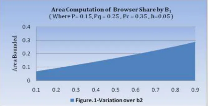
TABLE 1-[ For Figure (1) Where ( p =0.15, pq = 0.25, pc = 0.35, h=0.05) ]

b2 0.1 0.2 0.3 0.4 0.5 0.6 0.7 0.8 0.9

b1

_B

_B

_B

_B

_B

_B

_B

_B

_B

0 0.1389 0.1804 0.2218 0.2633 0.3047 0.3461 0.3876 0.429 0.4704

0.05 0.1324 0.1723 0.2125 0.2529 0.2936 0.3345 0.3756 0.4169 0.4585

0.1 0.1258 0.1642 0.2031 0.2424 0.2822 0.3224 0.3631 0.4043 0.4460

0.15 0.1191 0.156 0.1934 0.2316 0.2704 0.3099 0.3501 0.3910 0.4327

0.2 0.1124 0.1476 0.1836 0.2205 0.2583 0.2969 0.3366 0.3771 0.4187

0.25 0.1057 0.1392 0.1737 0.2092 0.2458 0.2835 0.3224 0.3625 0.4040





( ) ( ) 2( ... ) ...(4.1)

2

b b

n n

a a

h

I











1 ₁

2 1 2

(1 )(1 )

1 1 ...(3.1)

1 (1 )

q C

q

P P P b

B b P

b b P

    

    _{ } 

 

The generated data in above table for equal interval of b1 (here bounded area is defined by (A)): In

view of table 1 it is observe that at the fixed value of p =0.15 area (A) increase subject to the condition if we fixed pq = 0.25, pc = 0.35 and b2 increase with 0.1 interval .The minimum value of estimated area is 0.070 at b2

=0.1.

TABLE 2-[ For Figure (2) Where ( p

=0.35, b

= 0.25, p

= 0.45, h=0.05) ]

P 0.1 0.2 0.3 0.4 0.5 0.6 0.7 0.8 0.9

b1

_B

_B

_B

_B

_B

_B

_B

_B

_B

0 0.1354 0.1815 0.2276 0.2736 0.3197 0.3658 0.4118 0.4579 0.5039

0.05 0.1293 0.1733 0.2173 0.2613 0.3053 0.3493 0.3933 0.4373 0.4813

0.1 0.1232 0.1650 0.2070 0.2489 0.2908 0.3327 0.3746 0.4165 0.4584

0.15 0.117 0.1567 0.1965 0.2363 0.2761 0.3159 0.3557 0.3955 0.4352

0.2 0.1107 0.1483 0.1860 0.2236 0.2613 0.2989 0.3366 0.3742 0.4119

0.25 0.1043 0.1398 0.1753 0.2108 0.2463 0.2818 0.3172 0.3527 0.3882

0.3 0.0979 0.1312 0.1645 0.1978 0.2311 0.2644 0.2977 0.3310 0.3643

0.35 0.0914 0.1225 0.1536 0.1847 0.2158 0.2469 0.2780 0.3090 0.3401

0.4 0.0848 0.1137 0.1426 0.1714 0.2003 0.2291 0.2580 0.2868 0.3157

0.45 0.0782 0.1048 0.1314 0.158 0.1846 0.2112 0.2378 0.2644 0.2910

0.5 0.0715 0.0958 0.1201 0.1444 0.1688 0.1931 0.2174 0.2417 0.2660

0.55 0.0647 0.0867 0.1087 0.1307 0.1527 0.1747 0.1967 0.2188 0.2408

0.6 0.0578 0.0775 0.0972 0.1169 0.1365 0.1562 0.1759 0.1955 0.2152

0.65 0.0509 0.0682 0.0855 0.1028 0.1201 0.1374 0.1548 0.1721 0.1894

0.7 0.0439 0.0588 0.0737 0.0886 0.1036 0.1185 0.1334 0.1483 0.1633

0.75 0.0368 0.0492 0.0618 0.0743 0.0868 0.0993 0.1118 0.1243 0.1368

0.8 0.0296 0.0396 0.0497 0.0598 0.0698 0.0799 0.0900 0.1000 0.1101

0.85 0.0223 0.0299 0.0375 0.0451 0.0527 0.0603 0.0679 0.0755 0.0830

0.9 0.0150 0.0200 0.0251 0.0302 0.0353 0.0404 0.0455 0.0506 0.0557

0.95 0.0075 0.0100 0.0126 0.0152 0.0178 0.0203 0.0229 0.0254 0.0280

AREA(A)= 0.0700 0.0939 0.1177 0.1415 0.1653 0.1896 0.2130 0.2368 0.2606

In light of table 2 it is observe that maximum value of area is 0.2606 and minimum value is 0.0700 at fixed value of pq =0.35, b2= 0.25, pc = 0.45 and with little increment of interval 0.1of P.

0.3 0.0989 0.1307 0.1635 0.1976 0.2329 0.2696 0.3076 0.3472 0.3883

0.35 0.0921 0.122 0.1532 0.1857 0.2197 0.2551 0.2922 0.331 0.3716

0.4 0.0853 0.1133 0.1427 0.1736 0.206 0.2401 0.276 0.3139 0.3539

0.45 0.0784 0.1045 0.1320 0.1611 0.1919 0.2245 0.2591 0.2959 0.3351

0.5 0.0715 0.0956 0.1211 0.1483 0.1773 0.2082 0.2413 0.2768 0.3149

0.55 0.0645 0.0865 0.1100 0.1352 0.1622 0.1913 0.2226 0.2565 0.2934

0.6 0.0575 0.0774 0.0987 0.1217 0.1466 0.1736 0.203 0.2351 0.2703

0.65 0.0505 0.0681 0.0872 0.1079 0.1305 0.1552 0.1823 0.2122 0.2454

0.7 0.0434 0.0587 0.0755 0.0937 0.1138 0.136 0.1605 0.1879 0.2186

0.75 0.0363 0.0492 0.0635 0.0792 0.0965 0.1159 0.1375 0.1619 0.1896

0.8 0.0291 0.0396 0.0513 0.0642 0.0786 0.0948 0.1132 0.1341 0.1581

0.85 0.0219 0.0299 0.0388 0.0488 0.0601 0.0728 0.0874 0.1042 0.1239

0.9 0.0146 0.0201 0.0262 0.0330 0.0408 0.0497 0.0600 0.0721 0.0864

0.95 0.0073 0.0101 0.0132 0.0167 0.0208 0.0255 0.0310 0.0375 0.0453

TABLE 3-[ For Figure (3) Where ( p =0.45, b2= 0.15, pc = 0.25, h=0.05) ]

pq 0.1 0.2 0.3 0.4 0.5 0.6 0.7 0.8 0.9

b1

_B

_B

_B

_B

_B

_B

_B

_B

_B

0 0.3932 0.387 0.3808 0.3746 0.3684 0.3623 0.3561 0.3499 0.3437

0.05 0.3758 0.3694 0.3631 0.3569 0.3507 0.3446 0.3385 0.3325 0.3265

0.1 0.3582 0.3517 0.3453 0.339 0.3328 0.3268 0.3209 0.3151 0.3094

0.15 0.3404 0.3338 0.3273 0.321 0.3149 0.309 0.3033 0.2977 0.2922

0.2 0.3224 0.3157 0.3092 0.303 0.297 0.2912 0.2856 0.2802 0.275

0.25 0.3041 0.2974 0.291 0.2848 0.2789 0.2733 0.268 0.2628 0.2579

0.3 0.2856 0.2789 0.2726 0.2666 0.2608 0.2554 0.2503 0.2454 0.2407

0.35 0.2669 0.2603 0.2541 0.2482 0.2427 0.2375 0.2325 0.2279 0.2235

0.4 0.248 0.2415 0.2354 0.2297 0.2244 0.2195 0.2148 0.2104 0.2063

0.45 0.2288 0.2225 0.2166 0.2112 0.2061 0.2014 0.197 0.193 0.1892

0.5 0.2093 0.2033 0.1977 0.1925 0.1877 0.1833 0.1792 0.1755 0.172

0.55 0.1896 0.1839 0.1786 0.1737 0.1693 0.1652 0.1614 0.158 0.1548

0.6 0.1696 0.1643 0.1594 0.1549 0.1508 0.147 0.1436 0.1405 0.1376

0.65 0.1494 0.1445 0.14 0.1359 0.1322 0.1288 0.1257 0.1229 0.1204

0.7 0.1289 0.1245 0.1204 0.1168 0.1135 0.1105 0.1078 0.1054 0.1032

0.75 0.1082 0.1043 0.1008 0.0976 0.0948 0.0922 0.0899 0.0879 0.0860

0.8 0.0871 0.0838 0.0809 0.0783 0.076 0.0739 0.072 0.0703 0.0688

0.85 0.0658 0.0632 0.0609 0.0589 0.0571 0.0555 0.054 0.0528 0.0516

0.9 0.0441 0.0424 0.0408 0.0394 0.0381 0.037 0.036 0.0352 0.0344

0.95 0.0222 0.0213 0.0205 0.0197 0.0191 0.0185 0.018 0.0176 0.0172

AREA(A)= 0.2045 0.1994 0.1947 0.1902 0.1861 0.1821 0.1784 0.1748 0.1715

The table 3 shows that for p= 0.45 area (A) decreases subject to condition when b2= 0.15, pc = 0.25 and with the

little increment of of pq with interval 0.1.Minmum value is A 0.2045 for pq=0.1 and maximum value of A is

0.1715 for pq =0.9.

TABLE 4-[ For Figure (4) Where ( p =0.15, b2= 0.25, pq = 0.35, h=0.05) ]

Pc 0.1 0.2 0.3 0.4 0.5 0.6 0.7 0.8 0.9

b1

_B

_B

_B

_B

_B

_B

_B

_B

_B

0 0.2593 0.2305 0.2017 0.1729 0.1441 0.1153 0.0864 0.0576 0.0288

0.05 0.2477 0.2201 0.1926 0.1651 0.1376 0.1101 0.0826 0.055 0.0275

0.1 0.2359 0.2097 0.1835 0.1572 0.131 0.1048 0.0786 0.0524 0.0262

0.15 0.224 0.1991 0.1742 0.1493 0.1244 0.0995 0.0747 0.0498 0.0249

0.2 0.2119 0.1884 0.1648 0.1413 0.1177 0.0942 0.0706 0.0471 0.0235

0.25 0.1998 0.1776 0.1554 0.1332 0.111 0.0888 0.0666 0.0444 0.0222

0.3 0.1875 0.1666 0.1458 0.125 0.1041 0.0833 0.0625 0.0417 0.0208

0.35 0.175 0.1556 0.1361 0.1167 0.0972 0.0778 0.0583 0.0389 0.0194

0.4 0.1625 0.1444 0.1264 0.1083 0.0903 0.0722 0.0542 0.0361 0.0181

0.45 0.1497 0.1331 0.1165 0.0998 0.0832 0.0666 0.0499 0.0333 0.0166

0.5 0.1369 0.1217 0.1065 0.0913 0.076 0.0608 0.0456 0.0304 0.0152

0.55 0.1239 0.1101 0.0964 0.0826 0.0688 0.0551 0.0413 0.0275 0.0138

0.6 0.1107 0.0984 0.0861 0.0738 0.0615 0.0492 0.0369 0.0246 0.0123

0.65 0.0974 0.0866 0.0758 0.065 0.0541 0.0433 0.0325 0.0217 0.0108

0.7 0.084 0.0747 0.0653 0.056 0.0467 0.0373 0.028 0.0187 0.0093

0.75 0.0704 0.0626 0.0548 0.0469 0.0391 0.0313 0.0235 0.0156 0.0078

0.85 0.0427 0.038 0.0332 0.0285 0.0237 0.019 0.0142 0.0095 0.0047

0.9 0.0287 0.0255 0.0223 0.0191 0.0159 0.0127 0.0096 0.0064 0.0032

0.95 0.0144 0.0128 0.0112 0.0096 0.008 0.0064 0.0048 0.0032 0.0016

AREA(A)= 0.1341 0.1192 0.1043 0.0894 0.0745 0.0596 0.0447 0.0298 0.0149

In table 4 at the varying value of pc area (A) reduce for the constant value of p =0.15, b2= 0.25, pq =

0.35 .At pc =0.9 highest value of area is 0.0149 and lowest value is 0.1341 for pc=0.1

In view of figure 2 It is clear that estimated bounded area upward trend at variation over p and some fixed value b2= 0.25,Pq = 0.35 , Pc = 0.45 , h =0.05 where as figure3. Indicate downward trend of estimated

bounded area at variation over quieting probability pq and constant values Where P= 0.45,b2 = 0.15 , Pc =

0.25,which support table 3, 4 respectively.

In light of figure 4 It is observed that bounded area which estimated for variation over pc is downward

trend for some input fix values P= 0.15, b2 = 0.25, Pq = 0.35 which is supported by table 4.

Let us consider another form of integration for browser B2 defined as

 







2 2

1

2 2 2

1 2

(1

)

(1

)

1

1

...(5.2)

1

(1

)

u l u

q C

q l

I

f b db

P

P

P b

b

P

db

b b

P







_

 





_













_

_









_



_











The generated data in following table of equal interval of b2 are (A indicates estimated bounded area):

TABLE 5-[ For Figure (5) Where ( p =0.45, pc= 0.05, pq = 0.15, h=0.05) ]

b1 0.1 0.2 0.3 0.4 0.5 0.6 0.7 0.8 0.9

b2

_B

_B

_B

_B

_B

_B

_B

_B

_B

0 0.5588 0.5952 0.6315 0.6679 0.7042 0.7405 0.7769 0.8132 0.8495

0.05 0.5328 0.5695 0.6065 0.6438 0.6813 0.7191 0.7572 0.7955 0.8342

0.1 0.5066 0.5435 0.581 0.619 0.6575 0.6967 0.7364 0.7768 0.8178

0.15 0.4802 0.5171 0.5548 0.5934 0.6329 0.6732 0.7145 0.7568 0.8002

0.2 0.4536 0.4903 0.5281 0.5671 0.6072 0.6487 0.6914 0.7356 0.7812

0.25 0.4268 0.4631 0.5008 0.5399 0.5806 0.6229 0.667 0.7129 0.7608

0.3 0.3999 0.4355 0.4728 0.5119 0.5528 0.5959 0.6411 0.6887 0.7388

0.35 0.3727 0.4075 0.4442 0.483 0.524 0.5674 0.6136 0.6626 0.7149

0.4 0.3453 0.379 0.4149 0.4531 0.4939 0.5375 0.5843 0.6347 0.6889

0.45 0.3177 0.3501 0.3849 0.4222 0.4625 0.506 0.5532 0.6045 0.6605

0.5 0.2899 0.3208 0.3541 0.3903 0.4297 0.4727 0.5199 0.5719 0.6294

0.55 0.2619 0.291 0.3226 0.3573 0.3955 0.4376 0.4843 0.5365 0.5951

0.6 0.2337 0.2607 0.2904 0.3232 0.3596 0.4003 0.4461 0.498 0.5572

0.65 0.2052 0.2299 0.2573 0.2878 0.3221 0.3609 0.4051 0.4559 0.515

0.7 0.1766 0.1986 0.2233 0.2512 0.2828 0.3189 0.3608 0.4097 0.4678

0.75 0.1477 0.1669 0.1885 0.2132 0.2415 0.2743 0.3129 0.3589 0.4146

0.85 0.0893 0.1018 0.1161 0.1328 0.1524 0.1759 0.2044 0.2398 0.2849

0.9 0.0598 0.0684 0.0785 0.0903 0.1043 0.1214 0.1426 0.1695 0.2048

0.95 0.03 0.0345 0.0398 0.046 0.0536 0.063 0.0748 0.0902 0.1111

AREA(A)= 0.2856 0.3122 0.3404 0.3705 0.4029 0.4379 0.4761 0.5181 0.5650

Table 5 Shows that of variation over b2 in equal interval highest value of estimated bounded area (A) is 0.5650

for fixed value of p =0.45, pc= 0.05, pq = 0.15 and lowest value is 0.2856.

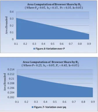
TABLE 6-[ For Figure (6) Where ( b1 =0.15, pc= 0.35, pq = 0.05, h=0.05) ]

P 0.1 0.2 0.3 0.4 0.5 0.6 0.7 0.8 0.9

b2

_B

_B

_B

_B

_B

_B

_B

_B

_B

0 0.5943 0.5385 0.4828 0.4271 0.3713 0.3156 0.2598 0.2041 0.1484

0.05 0.5684 0.5151 0.4618 0.4085 0.3552 0.3018 0.2485 0.1952 0.1419

0.1 0.5422 0.4913 0.4405 0.3896 0.3388 0.2879 0.2371 0.1862 0.1354

0.15 0.5156 0.4672 0.4189 0.3705 0.3222 0.2738 0.2254 0.1771 0.1287

0.2 0.4886 0.4428 0.397 0.3511 0.3053 0.2595 0.2137 0.1678 0.122

0.25 0.4613 0.418 0.3748 0.3315 0.2882 0.245 0.2017 0.1584 0.1152

0.3 0.4336 0.3929 0.3523 0.3116 0.2709 0.2303 0.1896 0.1489 0.1083

0.35 0.4055 0.3675 0.3294 0.2914 0.2534 0.2153 0.1773 0.1393 0.1012

0.4 0.377 0.3416 0.3063 0.2709 0.2355 0.2002 0.1648 0.1295 0.0941

0.45 0.348 0.3154 0.2828 0.2501 0.2175 0.1848 0.1522 0.1195 0.0869

0.5 0.3187 0.2888 0.2589 0.229 0.1991 0.1692 0.1394 0.1095 0.0796

0.55 0.2889 0.2618 0.2347 0.2076 0.1805 0.1534 0.1263 0.0992 0.0721

0.6 0.2587 0.2345 0.2102 0.1859 0.1617 0.1374 0.1131 0.0889 0.0646

0.65 0.2281 0.2067 0.1853 0.1639 0.1425 0.1211 0.0997 0.0783 0.0569

0.7 0.1969 0.1785 0.16 0.1415 0.1231 0.1046 0.0861 0.0676 0.0492

0.75 0.1654 0.1498 0.1343 0.1188 0.1033 0.0878 0.0723 0.0568 0.0413

0.8 0.1333 0.1208 0.1083 0.0958 0.0833 0.0708 0.0583 0.0458 0.0333

0.85 0.1007 0.0913 0.0818 0.0724 0.0629 0.0535 0.044 0.0346 0.0251

0.9 0.0677 0.0613 0.055 0.0486 0.0423 0.0359 0.0296 0.0232 0.0169

0.95 0.0341 0.0309 0.0277 0.0245 0.0213 0.0181 0.0149 0.0117 0.0085

AREA(A)= 0.3106 0.2815 0.2524 0.2232 0.1941 0.165 0.1358 0.1067 0.0776

In view of table 6 for constant value of b1 =0.15, pc= 0.35 and pq = 0.05 bounded area increase with fixed equal

interval of b2 and upper value of A is 0.3106 at p=0.1 and lowest value is 0.0776 for p=0.9.

TABLE 7-[ For Figure (7) Where ( b1 =0.05, p= 0.25, pc= 0.45, h=0.05) ]

pq 0.1 0.2 0.3 0.4 0.5 0.6 0.7 0.8 0.9

b2

_B

_B

_B

_B

_B

_B

_B

_B

_B

0 0.4187 0.418 0.4173 0.4166 0.4159 0.4153 0.4146 0.4139 0.4132

0.05 0.3986 0.3977 0.3969 0.3962 0.3954 0.3946 0.3939 0.3932 0.3925

0.1 0.3784 0.3774 0.3765 0.3756 0.3748 0.374 0.3733 0.3726 0.3719

0.15 0.3581 0.357 0.356 0.3551 0.3542 0.3534 0.3526 0.3519 0.3512

0.2 0.3377 0.3366 0.3355 0.3345 0.3336 0.3327 0.3319 0.3312 0.3306

0.25 0.3172 0.316 0.3149 0.3139 0.3129 0.3121 0.3113 0.3106 0.3099

0.3 0.2967 0.2954 0.2943 0.2932 0.2923 0.2914 0.2906 0.2899 0.2893

0.35 0.2761 0.2748 0.2736 0.2725 0.2715 0.2707 0.2699 0.2692 0.2686

0.45 0.2346 0.2333 0.2321 0.231 0.2301 0.2292 0.2285 0.2278 0.2273

0.5 0.2137 0.2124 0.2112 0.2102 0.2093 0.2085 0.2077 0.2071 0.2066

0.55 0.1927 0.1915 0.1904 0.1894 0.1885 0.1877 0.187 0.1864 0.186

0.6 0.1716 0.1705 0.1694 0.1685 0.1676 0.1669 0.1663 0.1657 0.1653

0.65 0.1505 0.1494 0.1484 0.1475 0.1468 0.1461 0.1455 0.145 0.1447

0.7 0.1293 0.1283 0.1274 0.1266 0.1259 0.1253 0.1248 0.1243 0.124

0.75 0.108 0.1071 0.1063 0.1056 0.105 0.1044 0.104 0.1036 0.1033

0.8 0.0865 0.0858 0.0851 0.0845 0.084 0.0836 0.0832 0.0829 0.0827

0.85 0.065 0.0645 0.0639 0.0635 0.0631 0.0627 0.0624 0.0622 0.062

0.9 0.0435 0.043 0.0427 0.0423 0.0421 0.0418 0.0416 0.0415 0.0413

0.95 0.0218 0.0216 0.0214 0.0212 0.021 0.0209 0.0208 0.0207 0.0207

AREA(A)= 0.2117 0.2107 0.2098 0.2090 0.2083 0.2077 0.2071 0.2066 0.2061

The table 7 shows that for increasing pq, the area A decreases subject to condition many other parametersb1, p,

pc are fixed. The highest value of area is as A=0.2117 at pq =0.1 whereas lowest value is A= 0.2061 on pq= 0.9.

TABLE 8-[ For Figure (8) Where ( b1 =0.35, p= 0.15, pq= 0.05, h=0.05) ]

Pc 0.1 0.2 0.3 0.4 0.5 0.6 0.7 0.8 0.9

b2

_B

_B

_B

_B

_B

_B

_B

_B

_B

0 0.8099 0.7199 0.6299 0.5399 0.4499 0.36 0.27 0.18 0.09

0.05 0.7817 0.6949 0.608 0.5212 0.4343 0.3474 0.2606 0.1737 0.0869

0.1 0.7527 0.669 0.5854 0.5018 0.4182 0.3345 0.2509 0.1673 0.0836

0.15 0.7226 0.6424 0.5621 0.4818 0.4015 0.3212 0.2409 0.1606 0.0803

0.2 0.6916 0.6148 0.5379 0.4611 0.3842 0.3074 0.2305 0.1537 0.0768

0.25 0.6595 0.5862 0.5129 0.4397 0.3664 0.2931 0.2198 0.1466 0.0733

0.3 0.6263 0.5567 0.4871 0.4175 0.3479 0.2783 0.2088 0.1392 0.0696

0.35 0.5919 0.5261 0.4603 0.3946 0.3288 0.263 0.1973 0.1315 0.0658

0.4 0.5562 0.4944 0.4326 0.3708 0.309 0.2472 0.1854 0.1236 0.0618

0.45 0.5192 0.4616 0.4039 0.3462 0.2885 0.2308 0.1731 0.1154 0.0577

0.5 0.4809 0.4275 0.374 0.3206 0.2672 0.2137 0.1603 0.1069 0.0534

0.55 0.4411 0.3921 0.3431 0.2941 0.245 0.196 0.147 0.098 0.049

0.6 0.3997 0.3553 0.3109 0.2665 0.2221 0.1776 0.1332 0.0888 0.0444

0.65 0.3567 0.3171 0.2774 0.2378 0.1982 0.1585 0.1189 0.0793 0.0396

0.7 0.3119 0.2773 0.2426 0.208 0.1733 0.1386 0.104 0.0693 0.0347

0.75 0.2653 0.2358 0.2064 0.1769 0.1474 0.1179 0.0884 0.059 0.0295

0.8 0.2168 0.1927 0.1686 0.1445 0.1204 0.0963 0.0723 0.0482 0.0241

0.85 0.1661 0.1476 0.1292 0.1107 0.0923 0.0738 0.0554 0.0369 0.0185

0.9 0.1132 0.1006 0.088 0.0754 0.0629 0.0503 0.0377 0.0251 0.0126

0.95 0.0579 0.0514 0.045 0.0386 0.0321 0.0257 0.0193 0.0129 0.0064

AREA(A)= 0.4544 0.4039 0.3534 0.3029 0.2524 0.2019 0.1515 0.1010 0.0505

The table 8 made on varying values of pc when many parameters are constant. Table 8 shows that for increasing

pc, the area A decreases subject to condition other parameters b1 =0.35, p= 0.15, pq= 0.05 are fixed. The highest

Fig 5 supports the facts observed in table 5 over variation of estimated bounded area A.

In light of figure 8 one can observe that estimated bounded area reduce for variation over quitting probability pc

for some constant parameter. And it supported with the help of table 8.

VI.

CONCLUSIONS

One can conclude that estimated bounded area (A) contains multitude of information about the browser sharing phenomenon. The area (A) is directly proportional to the browser selection probability (P) of users. Moreover, the bounded area is directly proportional to the browser failure probability. When browser failure probability of competitor browser increases, bounded area reduced. It provides the knowledge of relationship between browser selection probability (P) and browser failure probabilities b1 and b2 respectively.

REFERENCES

[1]. Catledge, L. D. and Pitkow J. E. (1995): Characterizing browsing strategies in the World-Wide Web., Computer Networks and ISDN Systems, 26 (6), pp. 55-65.

[2]. Deshpande, M. and Karypis G.(2004): Selective Markov Models for Predicting Web-Page Accesses., ACM Transactions on Internet Technology, Vol 4, No.2, May 2004,pp.168-184.

[3]. Yeian, and J. Lygeres (2005): Stabilization of a class of stochastic differential equations with markovian switching, System and Control Letters, issue 9, pp. 819-833.

[4]. Emanual Perzen(1992): “Stochastic Processes”, Holden-Day, Inc., San Francisco, and California. [5]. J. Medhi(1991):Stochastic Models in queuing theory, Academic Press Professional, Inc., San Diego,

CA.

[6]. M. Newby and R. Dagg (2002): Optical inspection and maintenance for stochastically deteriorating systems: average cost criteria, Jour. Ind. Stat. Asso., 40(2), pp169-198.

[7]. Aggarwal, R. and Dr. Kaur, L.(2008) :On Reliability Analysis of Fault-tolerant Multistage Interconnection Networks , International Journal of Computer Science and Security (IJCSS), 2(4),pp. 01-08.

[8]. Abuagla Babiker Mohd and Dr. Sulaiman bin Mohd Nor(2009) :Towards a Flow-based Internet Traffic Classification for Bandwidth Optimization, International Journal of Computer Science and Security (IJCSS), 3(2),pp.146-153.

[9]. Agarwal, Ankur (2009): System-Level Modeling of a Network-on-Chip, International Journal of Computer Science and Security (IJCSS), 3(3), pp.154-174.

[10]. Naldi, M. (2002): Internet access traffic sharing in a multi-user environment, Computer Networks. Vol. 38, pp. 809-824.

[11]. Shukla, D., Gangele, Sharad, Singhai, R., and Verma, Kapil (2011a): Elasticity analysis of web-browsing behavior of users, International Journal of Advanced Networking And Application (IJANA), Vol. 3 No.3, pp 1162- 1168.

[12]. Shukla, D. and Singhai, Rahul (2011b): Analysis of Users Web Browsing Behavior Using Markov chain Model, International Journal of Advanced Networking And Application (IJANA), Vol. 2 No.5, pp 824- 830.

[14]. Shukla, D. , Gangele , Sharad, Verma, Kapil and Singh, Pankaja (2011d): Elasticity and Index analysis of usual Internet traffic share problem, International Journal of Advanced Research in Computer Science(IJARCS), Vol. 02,no. 04 ,pp 473- 478.

[15]. Shukla, D., Gangele, Sharad, Verma, Kapil and Thakur, Sanjay (2011e) : A study on index based analysis of user of Internet traffic sharing in computer network, World Applied Programming (WAP), Vol. 1, no.04, pp 278- 287.

[16]. Shukla, D., Thakur, S. and Deshmukh, A. K. (2009a): State Probability Analysis of Internet Traffic Sharing in Computer Network, Int. Jour. of Advanced Networking and Applications, Vol. 1, Issue 2, pp 90-95.

[17]. Shukla, D. ,Tiwari, Virendra , Thakur ,S. and Deshmukh, A.K.( 2009b): Share loss analysis of Internet traffic distribution in computer network, International Journal of Computer Science and security (IJCSS) , Vol 3, Issue 5, pp 414 -427.

[18]. Shukla D., Tiwari, Virendra Kumar ,Thakur , S. and Tiwari, Mohan (2009c): A comparison of Methods for Internet Traffic Sharing in Computer Network, International Journal of Advanced Networking, (IJANA), Vol. 1, Issue 3, pp 164- 169.

[19]. Shukla, D., Verma, Kapil and Gangele, Sharad, (2012a): Least square based curve fitting in internet access traffic sharing in a two operator environment, International Journal of computer application (IJCA), Vol. 43, No. 12, pp. 26-32.

[20]. Shukla, D., Verma, Kapil and Gangele, Sharad, (2012b): Curve Fitting Approximation in Internet Traffic Distribution in Computer Network in Two Market Environment, International Journal of Computer Science and Information Security (IJCSIS), Vol. 10, Issue 05, pp. 71-78.

[21]. Shukla,D., Verma, Kapil and Gangele, Sharad, (2012c): Least Square Fitting Applications under Rest State Environment in Internet Traffic Sharing in Computer Network, International Journal of Computer Science and Telecommunications (IJCST), Vol.3, Issue 05, pp.43-51.