Data-Driven Graph Construction for Semi-Supervised Graph-Based
Learning in NLP
Andrei Alexandrescu
Dept. of Computer Science and Engineering University of Washington
Seattle, WA, 98195 [email protected]
Katrin Kirchhoff Dept. of Electrical Engineering
University of Washington Seattle, WA 98195 [email protected]
Abstract
Graph-based semi-supervised learning has recently emerged as a promising approach to data-sparse learning problems in natu-ral language processing. All graph-based algorithms rely on a graph that jointly rep-resents labeled and unlabeled data points. The problem of how to best construct this graph remains largely unsolved. In this paper we introduce a data-driven method that optimizes the representation of the initial feature space for graph construc-tion by means of a supervised classifier. We apply this technique in the frame-work of label propagation and evaluate it on two different classification tasks, a multi-class lexicon acquisition task and a word sense disambiguation task. Signifi-cant improvements are demonstrated over both label propagation using conventional graph construction and state-of-the-art su-pervised classifiers.
1 Introduction
Natural Language Processing (NLP) applications benefit from the availability of large amounts of an-notated data. However, such data is often scarce, particularly for non-mainstream languages. Semi-supervised learning addresses this problem by com-bining large amounts of unlabeled data with a small set of labeled data in order to learn a classifica-tion funcclassifica-tion. One class of semi-supervised learn-ing algorithms that has recently attracted increased
interest is graph-based learning. Graph-based tech-niques represent labeled and unlabeled data points as nodes in a graph with weighted edges encoding the similarity of pairs of samples. Various tech-niques are then available for transferring class la-bels from the labeled to the unlabeled data points. These approaches have shown good performance in cases where the data is characterized by an underly-ing manifold structure and samples are judged to be similar by local similarity measures. However, the question of how to best construct the graph forming the basis of the learning procedure is still an under-investigated research problem. NLP learning tasks present additional problems since they often rely on discrete or heterogeneous feature spaces for which standard similarity measures (such as Euclidean or cosine distance) are suboptimal.
We propose a two-pass data-driven technique for graph construction in the framework of label propa-gation (Zhu, 2005). First, we use a supervised clas-sifier trained on the labeled subset to transform the initial feature space (consisting of e.g. lexical, con-textual, or syntactic features) into a continuous rep-resentation in the form of soft label predictions. This representation is then used as a basis for measur-ing similarity among samples that determines the structure of the graph used for the second, semi-supervised learning step. It is important to note that, rather than simply cascading the supervised and the semi-supervised learner, we optimize the combina-tion with respect to the properties required of the graph. We present several techniques for such op-timization, including regularization of the first-pass classifier, biasing by class priors, and linear
nation of classifier predictions with known features. The proposed approach is evaluated on a lexicon learning task using the Wall Street Journal (WSJ) corpus, and on the SENSEVAL-3 word sense dis-ambiguation task. In both cases our technique sig-nificantly outperforms our baseline systems (label propagation using standard graph construction and discriminatively trained supervised classifiers).
2 Background
Several graph-based learning techniques have re-cently been developed and applied to NLP prob-lems: minimum cuts (Pang and Lee, 2004), random walks (Mihalcea, 2005; Otterbacher et al., 2005), graph matching (Haghighi et al., 2005), and label propagation (Niu et al., 2005). Here we focus on label propagation as a learning technique.
2.1 Label propagation
The basic label propagation (LP) algorithm (Zhu and Ghahramani, 2002; Zhu, 2005) has as inputs:
• a labeled set{(x1, y1),(x2, y2), . . . ,(xn, yn)}, wherexiare samples (feature vectors) andyi∈
{1,2, . . . , C}are their corresponding labels; • an unlabeled set{xn+1, . . . , xN};
• a distance measured(i, j)i, j ∈ {1, . . . N}
de-fined on the feature space.
The goal is to infer the labels {yn+1, . . . , yN} for the unlabeled set. The algorithm represents all N data points as vertices in an undirected graph with weighted edges. Initially, only the known data ver-tices are labeled. The edge linking verver-ticesiand j has weight:
wij= exp
−d(i, j) 2
α2
(1) whereαis a hyperparameter that needs to be empir-ically chosen or learned separately. wijindicates the label affinity of vertices: the largerwijis, the more likely it is thatiandj have the same label. The LP algorithm constructs a row-normalizedN×N tran-sition probability matrixP as follows:
Pij =P(i→j) = PNwij
k=1wik
(2)
The algorithm probabilistically pushes labels from the labeled nodes to the unlabeled nodes. To do so, it defines then×Chard labels matrixY and theN×C soft labels matrixf, whose firstnrows are identical toY. The hard labels matrixY is invariant through
the algorithm and is initialized with probability 1 for the known label and 0 for all other labels:
Yic=δ(yi, C) (3) where δ is Kronecker’s delta function. The algo-rithm iterates as follows:
1. f0 ←P ×f
2. f[0rows1 to n]←Y 3. Iff0 ∼=f, stop
4. f ←f0
5. Repeat from step 1
In each iteration, step 2 fixes the known labels, which might otherwise be overriden by propagated labels. The resulting labels for each feature xi, wherei∈ {n+ 1, . . . , N}, are:
li = arg max j=1,...,C
fij (4)
It is important that the distance measure is locally accurate, i.e. nodes connected by an edge with a high weight should have the same label. The global distance is less relevant since label information will be propagated from labeled points through the entire space. This is why LP works well with a local dis-tance measure that might be unsuitable as a global distance measure.
Applications of LP include handwriting recogni-tion (Zhu and Ghahramani, 2002), image classifi-cation (Balcan et al., 2005) and retrieval (Qin et al., 2005), and protein classification (Weston et al., 2003). In NLP, label propagation has been used for word sense disambiguation (Niu et al., 2005), doc-ument classification (Zhu, 2005), sentiment analy-sis (Goldberg and Zhu, 2006), and relation extrac-tion (Chen et al., 2006).
2.2 Graph construction
distance likewise assumes that the different feature vector dimensions are uncorrelated. However, many applications, particularly in NLP, rely on feature spaces with correlated dimensions. Moreover, fea-tures may have different ranges and different types (e.g. continuous, binary, multi-valued), which en-tails the need for normalization, binning, or scaling. Finally, common distance measures do not take ad-vantage of domain knowledge that might be avail-able.
Some attempts have been made at improving the standard method of graph construction. For in-stance, in a face identification task (Balcan et al., 2005), domain knowledge was used to identify three different edge sets based on time, color and face features, associating a different hyperparameter with each. The resulting graph was then created by super-posing edge sets. Zhu (Zhu, 2005, Ch. 7) describes graph construction using separate α hyperparame-ters for each feature dimension, and presents a data-driven way (evidence maximization) for learning the values of the parameters.
3 Data-driven graph construction
Unlike previous work, we propose to optimize the feature representation used for graph construction by learning it with a first-pass supervised classi-fier. Under this approach, similarity of samples is defined as similarity of the output values produced by a classifier applied to the original feature repre-sentation of the samples. This idea bears similar-ity to classifier cascading (Alpaydin and Kaynak, 1998), where classifiers are trained around a rule-exceptions paradigm; however, in our case, the clas-sifiers work together, the first acting as a jointly op-timized feature mapping function for the second.
1. Train a first-pass supervised classifier that out-puts soft label predictions Zi for all sam-ples i ∈ {1, . . . N}, e.g. a posterior
prob-ability distribution over target labels: Zi =
hpi1, pi2, . . . , piCi;
2. Apply postprocessing toZiif needed.
3. Use vectorsZiand an appropriately chosen dis-tance measure to construct a graph for LP. 4. Perform label propagation over the constructed
graph to find the labeling of the test samples. The advantages of this procedure are:
• Uniform range and type of features: The
out-put from a first-pass classifier can produce well-defined features, e.g. posterior probability distribu-tions. This eliminates the problem of input features of different ranges and types (e.g. binary vs. multi-valued, continuous vs. categorical attributes) which are often used in combination.
• Feature postprocessing: The transformation of
features into a different space also opens up pos-sibilities for postprocessing (e.g. probability distri-bution warping) depending on the requirements of the second-pass learner. In addition, different dis-tance functions (e.g. those defined on probability spaces) can be used, which avoids violating assump-tions made by metrics such as Euclidean and cosine distance.
• Optimizing class separation: The learned repre-sentation of labeled training samples might reveal better clusters in the data than the original represen-tation: a discriminatively-trained first pass classifier will attempt to maximize the separation of samples belonging to different classes. Moreover, the first-pass classifier may learn a feature transformation that suppresses noise in the original input space. Difficulties with the proposed approach might arise when the first-pass classifier yields confident but wrong predictions, especially for outlier samples in the original space. For this reason, the first-pass classifier and the graph-based learner should not simply be concatenated without modification, but the first classifier should be optimized with respect to the requirements of the second. In our case, the choice of first-pass classifier and joint optimization techniques are determined by the particular learning task and are detailed below.
4 Tasks
4.1 Lexicon acquisition task
lexi-cons are one of the most basic language resources, which enable subsequent training of taggers, chun-kers, etc. We assume that a small set of words can be reliably annotated, and that POS-sets for the remain-ing words can be inferred by semi-supervised learn-ing. Rather than choosing a genuinely resource-poor language for this task, we use the English Wall Street Journal (WSJ) corpus and artificially limit the size of the labeled set. This is because the WSJ corpus is widely obtainable and allows easy replication of our experiments.
We use sections 0-18 of the Wall Street Journal corpus (N = 44,492). Words have between 1 and
4 POS tags, with an average of 1.1 per word. The number of POS tags is 36, and we treat every POS combination as a unique class, resulting inC = 158
distinct labels. We use three different randomly se-lected training sets of various sizes: 5000, 10000, and 15000 words, representing about 11%, 22%, and 34% of the entire data set respectively; the rest of the data was used for testing. In order to avoid experi-mental bias, we run all experiments on five differ-ent randomly chosen labeled subsets and report av-erages and standard deviations. Due to the random sampling of the data it is possible that some labels never occur in the training set or only occur once. We train our classifiers only on those labels that oc-cur at least twice, which results in 60-63 classes. La-bels not present in the training set will therefore not be hypothesized and are guaranteed to be errors. We delete samples with unknown labels from our unla-beled set since their percentage is less than 0.5% on average.
We use the following features to represent sam-ples:
• Integer: the three-letter suffix of the word; • Integer: The four-letter suffix of the word; • Integer×4: The indices of the four most
fre-quent words that immediately precede the word in the WSJ text;
• Boolean: word contains capital letters; • Boolean: word consists only of capital letters; • Boolean: word contains digits;
• Boolean: word contains a hyphen;
• Boolean: word contains other special
charac-ters (e.g. “&”).
We have also experimented with shorter suffixes and with prefixes but those features tended to degrade
performance.
4.2 SENSEVAL-3 word sense disambiguation task
The second task is word sense disambiguation using the SENSEVAL-3 corpus (Mihalcea et al., 2004), to enable a comparison of our method with previously published results. The goal is to disambiguate the different senses of each of 57 words given the sen-tences within which they occur. There are 7860 sam-ples for training and 3944 for testing. In line with existing work (Lee and Ng, 2002; Niu et al., 2005), we use the following features:
• Integer × 7: seven features consisting of the
POS of the previous three words, the POS of the next three words, and the POS of the word itself. We used the MXPOST tagger (Ratna-parkhi, 1996) for POS annotation.
• Integer×hvariable lengthi: a bag of all words in the surrounding context.
• Integer×15: Local collocations Cij (i, j are the bounds of the collocation window)—word combinations from the context of the word to disambiguate. In addition to the 11 collocations used in similar work (Lee and Ng, 2002), we also usedC−3,1,C−3,2,C−2,3,C−1,3.
Note that syntactic features, which have been used in some previous studies on this dataset (Mohammad and Pedersen, 2004), were not included. We apply a simple feature selection method: a featureX is se-lected if the conditional entropy H(Y|X) is above
a fixed threshold (1 bit) in the training set, and ifX also occurs in the test set (note that no label infor-mation from the test data is used for this purpose).
5 Experiments
For both tasks we compare the performance of a su-pervised classifier, label propagation using the stan-dard input features and either Euclidean or cosine distance, and LP using the output from a first-pass supervised classifier.
5.1 Lexicon acquisition task 5.1.1 First-pass classifier
con-x2
x4
x1
x3
P(y | x)
M
i
h
o
Wih W
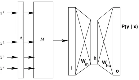
[image:5.612.74.298.57.187.2]ho A
Figure 1: Architecture of first-pass supervised classifier (MLP) for lexicon acquisition
.
tinuous values by a discrete-to-continuous mapping layer M, which is itself learned during the MLP training process. This layer connects to the hidden layer h, which in turn is connected to the output layero. The entire network is trained via backprop-agation. The training criterion maximizes the regu-larized log-likelihood of the training data:
L= 1
n n
X
t=1
logP(yt|xt, θ) +R(θ) (5)
The use of an additional continuous mapping layer is similar to the use of hidden continuous word rep-resentations in neural language modeling (Bengio et al., 2000) and yields better results than a standard 3-layer MLP topology.
Problems caused by data scarcity arise when some of the input features of the unlabeled words have never been seen in the training set, resulting in un-trained, randomly-initialized values for those fea-ture vector components. We address this problem by creating an approximation layer Athat finds the known input feature vector x0 that is most similar to x (by measuring the cosine similarity between the vectors). Thenxkis replaced withx0k, resulting in vectorxˆ=hx1, . . . , xk−1, x0k, xk+1, . . . , xfithat has no unseen features and is closest to the original vector.
5.1.2 LP Setup
We use a dense graph approach. The WSJ set has a total of 44,492 words, therefore the P ma-trix that the algorithm requires would have44,492×
44,492 ∼= 2×10⁹elements. Due to the matrix size,
we avoid the analytical solution of the LP problem, which requires inverting theP matrix, and choose
the iterative approach described above (Sec. 2.1) in-stead. Convergence is stopped when the maximum relative difference between each cell of f and the corresponding cell off0is less than 1%.
Also for data size reasons, we apply LP in chunks. While the training set stays in memory, the test data is loaded in fixed-size chunks, labeled, and dis-carded. This approach has yielded similar results for various chunk sizes, suggesting that chunking is a good approximation of whole-set label propaga-tion.1 LP in chunks is also amenable to
paralleliza-tion: Our system labels different chunks in parallel. We trained the α hyperparameter by three-fold cross-validation on the training data, using a geo-metric progression with limits 0.1and 10 and ratio 2. We set fixed upper limits of edges between an
unlabeled node and its labeled neighbors to15, and
between an unlabeled node and its unlabeled neigh-bors to5. The approach of setting different limits
among different kinds of nodes is also used in re-lated work (Goldberg and Zhu, 2006).
For graph construction we tested: (a) the original discrete input representation with cosine distance; (b) the classifier output features (probability distri-butions) with the Jeffries-Matusita distance.
5.2 Combination optimization
The static parameters of the MLP (learning rate, reg-ularization rate, and number of hidden units) were optimized for the LP step by 5-fold cross-validation on the training data. This process is important be-cause overspecialization is detrimental to the com-bined system: an overspecialized first-pass classi-fier may output very confident but wrong predic-tions for unseen patterns, thus placing such samples at large distances from all correctly labeled sam-ples. A strongly regularized neural network, by con-trast, will output smoother probability distributions for unseen patterns. Such outputs also result in a smoother graph, which in turn helps the LP process. Thus, we found that a network with only 12 hidden units and relatively highR(θ)in Eq. 5 (10% of the
weight value) performed best in combination with LP (at an insignificant cost in accuracy when used
1In fact, experiments have shown that performance tends to
as an isolated classifier).
5.2.1 Results
We first conducted an experiment to measure the smoothness of the underlying graph, S(G), in the two LP experiments according to the following for-mula: S(G) = X
yi6=yj,(i>n∨j>n)
wij (6)
whereyiis the label of samplei. (Lower values are better as they reflect less affinity between nodes of different labels.) The value ofS(G)was in all cases
significantly better on graphs constructed with our proposed technique than on graphs constructed in the standard way (see Table 1). Table 1 also shows the performance comparison between LP over the discrete representation and cosine distance (“LP”), the neural network itself (“NN”), and LP over the continuous representation (“NN+LP”), on all dif-ferent subsets and for difdif-ferent training sizes. For scarce labeled data (5000 samples) the neural net-work, which uses a strictly supervised training pro-cedure, is at a clear disadvantage. However, for a larger training set the network is able to perform more accurately than the LP learner that uses the discrete features directly. The third, combined tech-nique outperforms the first two significantly.2 The
differences are more pronounced for smaller train-ing set sizes. Interesttrain-ingly, the LP is able to extract information from largely erroneous (noisy) distribu-tions learned by the neural network.
5.3 Word Sense Disambiguation
We compare the performance of an SVM classifier, an LP learner using the same input features as the SVM, and an LP learner using the SVM outputs as input features. To analyze the influence of train-ing set size on accuracy, we randomly sample sub-sets of the training data (25%, 50%, and 75%) and use the remaining training data plus the test data as unlabeled data, similarly to the procedure fol-lowed in related work (Niu et al., 2005). The re-sults are averaged over five different random sam-plings. The samplings were chosen such that there was at least one sample for each label in the training set. SENSEVAL-3 sports multi-labeled samples and 2Significance was tested using a difference of proportions
significance test; the significance level is 0.01 or smaller in all cases.
samples with the “unknown” label. We eliminate all samples labeled as unknown and retain only the first label for the multi-labeled instances.
5.3.1 SVM setup
The use of SVM vs. MLP in this case was justi-fied by the very small training data set. An MLP has many parameters and needs a considerable amount of data for effective training, so for this task with only on the order of102training samples per
classi-fier, an SVM was deemed more appropriate. We use the SVMlight package to build a set of binary clas-sifiers in a one-versus-all formulation of the multi-class multi-classification problem. The features input to each SVM consist of the discrete features described above (Sec. 4.2) after feature selection. After train-ing SVMs for each target label against the union of all others, we evaluate the SVM approach against the test set by using the winner-takes-all strategy: the predicted label corresponds to the SVM that outputs the largest value.
5.3.2 LP setup
Again we set up two LP systems: one using the original feature space (after feature selection, which benefited all of the tested systems) and one using the SVM outputs. Both use a cosine distance measure. The α parameter (see Eq. 1) is optimized through 3-fold cross-validation on the training set.
5.4 Combination optimization
Unlike MLPs, SVMs do not compute a smooth out-put distribution but base the classification decision on the sign of the output values. In order to smooth output values with a view towards graph construc-tion we applied the following techniques:
1. Combining SVM predictions and perfect fea-ture vectors: After training, the SVM actu-ally outputs wrong label predictions for a small number (≈5%) of training samples. These
Initial labels Model S(G)avg. Accuracy (%)
Set 1 Set 2 Set 3 Set 4 Set 5 Average
5000 NN − 50.70 59.22 63.77 60.09 54.58 57.67±4.55
LP 451.54 58.37 59.91 60.88 62.01 59.47 60.13±1.24
NN+LP 409.79 58.03 63.91 66.62 65.93 57.76 62.45±3.83
10000 NN − 65.86 60.19 67.52 65.68 65.64 64.98±2.49
LP 381.16 58.27 60.04 60.85 61.99 62.06 60.64±1.40
NN+LP 315.53 69.36 64.73 69.50 70.26 67.71 68.31±1.97
15000 NN − 69.85 66.42 70.88 70.71 72.18 70.01±1.94
LP 299.10 58.51 61.00 60.94 63.53 60.98 60.99±1.59
[image:7.612.319.534.324.422.2]NN+LP 235.83 70.59 69.45 69.99 71.20 73.45 70.94±1.39
Table 1: Accuracy results of neural classification (NN), LP with discrete features (LP), and combined (NN+LP), over 5 random samplings of 5000, 10000, and 15000 labeled words in the WSJ lexicon acquisition task.S(G)is the smoothness of the graph
vectorsvthat contain 1 at the correct label po-sition and -1 elsewhere:
s0i =γsi+ (1−γ)vi (7) wheresi,s0iare the i’th input and output feature vectors andγ a parameter fixed at 0.5.
2. Biasing uninformative distributions: For some training samples, although the predicted class label was correct, the outputs of the SVM were relatively close to one another, i.e. the decision was borderline. We decided to bias these SVM outputs in the right direction by using the same formula as in equation 7.
3. Weighting by class priors: For each training sample, a corresponding sample with the per-fect output features was added, thus doubling the total number of labeled nodes in the graph. These synthesized nodes are akin to the “don-gle” nodes (Goldberg and Zhu, 2006). The dif-ference is that, while dongle nodes are only linked to one node, our artificial nodes are treated like any other node and as such can con-nect to several other nodes. The role of the arti-ficial nodes is to serve as authorities during the LP process and to emphasize class priors.
5.4.1 Results
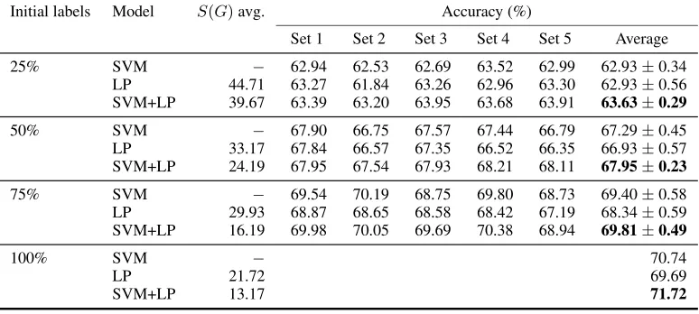
As before, we measured the smoothness of the graphs in the two label propagation setups and found that in all cases the smoothness of the graph pro-duced with our method was better when compared to the graphs produced using the standard approach, as shown in Table 3, which also shows accuracy re-sults for the SVM (“SVM” label), LP over the stan-dard graph (“LP”), and label propagation over SVM outputs (“SVM+LP”). The latter system consistently
performs best in all cases, although the most marked gains occur in the upper range of labeled samples percentage. The gain of the best data-driven LP over the knowledge-based LP is significant in the 100% and 75% cases.
# System Acc. (%)
1 htsa3 (Grozea, 2004) 72.9
2 IRST-kernels (Strapparava et al., 2004) 72.6
3 nusels (Lee et al., 2004) 72.4
4 SENSEVAL-3 contest baseline 55.2
5 Niu et al. (Niu et al., 2005) LP/J-S 70.3
6 Niu et al. LP/cosine 68.4
7 Niu et al. SVM 69.7
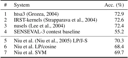
Table 2: Accuracy results of other published systems on SENSEVAL-3. 1-3 use syntactic features; 5-7 are directly com-parably to our system.
For comparison purposes, Table 2 shows results of other published systems against the SENSEVAL corpus. The “htsa3”, “IRST-kernels”, and “nusels” systems were the winners of the SENSEVAL-3 con-test and used extra input features (syntactic rela-tions). The Niu et al. work (Niu et al., 2005) is most comparable to ours. We attribute the slightly higher performance of our SVM due to our feature selection process. The LP/cosine system is a system similar to our LP system using the discrete features, and the LP/Jensen-Shannon system is also similar but uses a distance measure derived from Jensen-Shannon divergence.
6 Conclusions
first-Initial labels Model S(G)avg. Accuracy (%)
Set 1 Set 2 Set 3 Set 4 Set 5 Average
25% SVM − 62.94 62.53 62.69 63.52 62.99 62.93±0.34
LP 44.71 63.27 61.84 63.26 62.96 63.30 62.93±0.56
SVM+LP 39.67 63.39 63.20 63.95 63.68 63.91 63.63±0.29
50% SVM − 67.90 66.75 67.57 67.44 66.79 67.29±0.45
LP 33.17 67.84 66.57 67.35 66.52 66.35 66.93±0.57
SVM+LP 24.19 67.95 67.54 67.93 68.21 68.11 67.95±0.23
75% SVM − 69.54 70.19 68.75 69.80 68.73 69.40±0.58
LP 29.93 68.87 68.65 68.58 68.42 67.19 68.34±0.59
SVM+LP 16.19 69.98 70.05 69.69 70.38 68.94 69.81±0.49
100% SVM − 70.74
LP 21.72 69.69
[image:8.612.113.500.61.235.2]SVM+LP 13.17 71.72
Table 3: Accuracy results of support vector machine (SVM), label propagation over discrete features (LP), and label propagation over SVM outputs (SVM+LP), each trained with 25%, 50%, 75% (5 random samplings each), and 100% of the train set. The improvements of SVM+LP are significant over LP in the 75% and 100% cases.S(G)is the graph smoothness
pass supervised classifier. The outputs from this classifier (especially when optimized for the second-pass learner) were shown to serve as a better repre-sentation for graph-based semi-supervised learning. Classification results on two learning tasks showed significantly better performance compared to LP us-ing standard graph construction and the supervised classifier alone.
Acknowledgments This work was funded by
NSF under grant no. IIS-0326276. Any opinions, findings and conclusions, or recommendations ex-pressed herein are those of the authors and do not necessarily reflect the views of this agency.
References
E. Alpaydin and C. Kaynak. 1998. Cascading classifiers. Ky-bernetika, 34:369–374.
Balcan et al. 2005. Person identification in webcam images. In
ICML Workshop on Learning with Partially Classified Train-ing Data.
Y. Bengio, R. Ducharme, and P. Vincent. 2000. A neural prob-abilistic language model. InNIPS.
J. Chen, D. Ji, C.L. Tan, and Z. Niu. 2006. Relation Extraction Using Label Propagation Based Semi-supervised Learning. InProceedings of ACL, pages 129–136.
A. Goldberg and J. Zhu. 2006. Seeing stars when there aren’t many stars: Graph-based semi-supervised learning for sen-timent categorization. InHLT-NAACL Workshop on Graph-based Algorithms for Natural Language Processing. C. Grozea. 2004. Finding optimal parameter settings for high
performance word sense disambiguation. Proceedings of Senseval-3 Workshop.
A. Haghighi, A. Ng, and C.D. Manning. 2005. Robust textual inference via graph matching. Proceedings of EMNLP. Y.K. Lee and H.T. Ng. 2002. An empirical evaluation of
knowl-edge sources and learning algorithms for word sense disam-biguation. InProceedings of EMNLP, pages 41–48.
Y.K. Lee, H.T. Ng, and T.K. Chia. 2004. Supervised Word Sense Disambiguation with Support Vector Machines and Multiple Knowledge Sources. SENSEVAL-3.
R. Mihalcea, T. Chklovski, and A. Killgariff. 2004. The Senseval-3 English Lexical Sample Task. InProceedings of ACL/SIGLEX Senseval-3.
R. Mihalcea. 2005. Unsupervised large-vocabulary word sense disambiguation with graph-based algorithms for sequence data labeling. InProceedings of HLT/EMNLP, pages 411– 418.
S. Mohammad and T. Pedersen. 2004. Complementarity of Lexical and Simple Syntactic Features: The SyntaLex Ap-proach to Senseval-3.Proceedings of the SENSEVAL-3. Zheng-Yu Niu, Dong-Hong Ji, and Chew Lim Tan. 2005. Word
sense disambiguation using label propagation based semi-supervised learning. InACL ’05.
J. Otterbacher, G. Erkan, and D.R. Radev. 2005. Using Ran-dom Walks for Question-focused Sentence Retrieval. Pro-ceedings of HLT/EMNLP, pages 915–922.
B. Pang and L. Lee. 2004. A sentimental education: Sen-timent analysis using subjectivity summarization based on minimum cuts. InProceedings of ACL, pages 271–278. T. Qin, T.-Y. Liu, X.-D. Zhang, W.-Y. Ma, and H.-J. Zhang.
2005. Subspace clustering and label propagation for active feedback in image retrieval. InMMM, pages 172–179. A. Ratnaparkhi. 1996. A maximum entropy model for
part-of-speech tagging. InProceedings of EMNLP, pages 133–142. C. Strapparava, A. Gliozzo, and C. Giuliano. 2004. Pattern
abstraction and term similarity for word sense disambigua-tion: IRST at SENSEVAL-3. Proc. of SENSEVAL-3, pages 229–234.
J. Weston, C. Leslie, D. Zhou, A. Elisseeff, and W. Noble. 2003. Semi-supervised protein classification using cluster kernels.
X. Zhu and Z. Ghahramani. 2002. Learning from labeled and unlabeled data with label propagation. Technical report, CMU-CALD-02.