Journal of Engineering Sciences, Volume 6, Issue 2 (2019), pp. A 1–A 7 A 1 JOURNAL OF ENGINEERING SCIENCES
ЖУРНАЛ ІНЖЕНЕРНИХ НАУК
ЖУРНАЛ ИНЖЕНЕРНЫХ НАУК
Web site: http://jes.sumdu.edu.ua DOI: 10.21272/jes.2019.6(2).a1/ Volume 6, Issue 2 (2019)
Simplified Grinding Temperature Model Study
Lishchenko N. V.1*, Larshin V. P.2, Krachunov H.3
1 Odessa National Academy of Food Technologies, 112 Kanatna St., 65039 Odessa, Ukraine; 2 Odessa National Polytechnic University, 1 Shevchenko Ave., 65044 Odessa, Ukraine;
3 University of Varna, Studentska Str., Varna, 9010, Bulgaria
Article info: Paper received:
The final version of the paper received: Paper accepted online:
June 12, 2019 September 3, 2019 September 8, 2019
*Corresponding Author’s Address:
[email protected]
Abstract. A study of a simplified mathematical model for determining the grinding temperature is performed. According to the obtained results, the equations of this model differ slightly from the corresponding more exact solution of the one-dimensional differential equation of heat conduction under the boundary conditions of the second kind. The model under study is represented by a system of two equations that describe the grinding temperature at the heating and cooling stages without the use of forced cooling. The scope of the studied model corresponds to the modern technological operations of grinding on CNC machines for conditions where the numerical value of the Peclet number is more than 4. This, in turn, corresponds to the Jaeger criterion for the so-called fast-moving heat source, for which the operation parameter of the workpiece velocity may be equivalently (in temperature) replaced by the action time of the heat source. This makes it possible to use a simpler solution of the one-dimensional differential equation of heat conduction at the boundary conditions of the second kind (one-dimensional analytical model) instead of a similar solution of the two-dimensional one with a slight deviation of the grinding temperature calculation result. It is established that the proposed simplified mathematical expression for determining the grinding temperature differs from the more accurate one-dimensional analytical solution by no more than 11 % and 15 % at the stages of heating and cooling, respectively. Comparison of the data on the grinding temperature change according to the conventional and developed equations has shown that these equations are close and have two points of coincidence: on the surface and at the depth of approximately threefold decrease in temperature. It is also established that the nature of the ratio between the scales of change of the Peclet number 0.09 and 9 and the grinding temperature depth 1 and 10 is of 100 to 10. Additionally, another unusual mechanism is revealed for both compared equations: a higher temperature at the surface is accompanied by a lower temperature at the depth.
Keywords: grinding temperature, heating stage, cooling stage, dimensionless temperature, temperature model.
1
Introduction
Abrasive machining works by forcing the abrasive par-ticles, or grains, into the surface of the workpiece so that each particle cuts away a small bit of material. Abrasive machining is similar to conventional machining (metal cutting), such as milling or turning, because each of the abrasive particles acts like a miniature cutting tool. How-ever, unlike conventional machining, the grains are much smaller than a cutting tool, and the geometry and orienta-tion of individual grains are not well defined. As a result, abrasive machining is less power efficient and generates more heat. The grain size may be different based on the machining. For rough grinding, coarse abrasives are used. For fine grinding, fine grains (abrasives) are used.
Abrasive machining processes can be divided into two categories based on how the grains are applied to the workpiece.
In bonded abrasive processes, the particles are held to-gether within a matrix, and their combined shape deter-mines the geometry of the finished workpiece. For exam-ple, in grinding the particles are bonded together in a wheel. As the grinding wheel is fed into the part, its shape is transferred onto the workpiece.
A 2 MANUFACTURING ENGINEERING: Machines and Tools Common abrasive processes are listed below. Fixed
(bonded) abrasive processes: grinding, honing, superfin-ishing, tape finsuperfin-ishing, abrasive belt machining, abrasive sawing, diamond wire cutting, wire saw sanding.
Loose abrasive processes: polishing, lapping, abrasive flow machining (AFM), hydro-erosive grinding, water-jet cutting, abrasive blasting mass finishing, tumbling, open barrel tumbling, vibratory bowl tumbling, centrifugal disc tumbling, centrifugal barrel tumbling.
Grinding is an abrasive machining process that uses a grinding wheel as the cutting tool. Grinding practice is a large and diverse area of manufacturing and tool making. It can produce very fine finishes and very accurate di-mensions. At the same time, in mass production, it can also rough out large volumes of metal quite rapidly. It is usually better suited to the machining of very hard mate-rials than is "regular" machining (that is, cutting larger chips with cutting tools such as tool bits or milling cut-ters), and until recent decades it was the only practical way to machine such materials as hardened steels. Com-pared to “regular” machining, it is usually better suited to taking very shallow cuts, such as reducing a shaft’s diam-eter by half a thousandth of an inch or 12.7 μm.
Grinding is a subset of cutting, as grinding is a true metal-cutting process. Each grain of abrasive functions as a microscopic single-point cutting edge (although of high negative rake angle) and shears a tiny chip that is analo-gous to what would conventionally be called a “cut” chip (turning, milling, drilling, tapping, etc.). However, among people who work in the machining fields, the term cutting is often understood to refer to the macroscopic cutting operations, and grinding is often mentally categorized as a "separate" process (abrasive machining). This is why the terms (“grinding” and “metal cutting”) are usually used separately in shop-floor practice.
The designing, monitoring and diagnosing computer subsystems are widely used on CNC grinding machines to adapt the grinding system to higher throughput. Abra-sive machining compared with metal cutting is more labor-intensive and costly. That is why the grinding sys-tem study is caused by the search for ways to improve the productivity of man and machine [1]. In this connection, there is some modern knowledge to boost the grinding system throughput. This knowledge is more important with automated computer-controlled systems than it has ever been before because quantitative knowledge is need-ed to design and operate these systems [2].
By means of electrical signals from sensors, you can judge the state of the machine under control and the envi-ronment. Therefore, the more sensors used, the more information you can be obtained about the grinding sys-tem and environment. However, it should be borne in mind that in real conditions there is such information which is impossible directly to take off with the help of sensors.
This situation may occur, for example, when the measured signal is distorted by noise or the controlled value cannot be converted to an electrical signal as well as when due to cost or spatial constraints you cannot use the required sensor. If in such cases the noise properties or dynamic characteristics of the object, which are held observations, are known then with the help of appropriate calculations you can evaluate the signal you are interested in [3].
This situation fully applies to the grinding temperature signal in the grinding zone which is located between a grinding wheel and a workpiece to be ground. For this reason, the development of an acceptable mathematical model for determining the grinding temperature is an urgent task in the grinding technology on CNC machines. In terms of metrology, such solution to the problem is an example of indirect measurement. This opens the way to building “hierarchically intelligent control systems” de-veloped by Sarid is on the basis of his principle of “in-creasing precision with de“in-creasing intelligence” [4]. All this mentioned above ultimately predetermines the devel-opment of the main industries in developed countries [5] and corresponds to the so-called tendency of “sustainable development”.
2
Literature Review
Journal of Engineering Sciences, Volume 6, Issue 2 (2019), pp. A 1–A 7 A 3
3
Research Methodology
3.1 Mathematical model
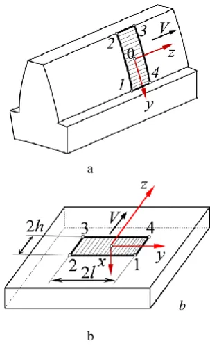
In the grinding theory, the contact spot is usually con-sidered as a certain zone on the surface to be ground, which belongs to both the grinding wheel and the work-piece (Figure 1).
a
b
Figure 1 – Schemes of profile gear grinding (a) and flat grinding (b) with the discrete radial feed ae of the grinding
wheel to the workpiece
From the grinding thermal physics point of view, these schemes can be converted into the so-called moving heat source, indicated by the numbers 1234 in Figure 2.
a
b
Figure 2 – Real (a) and equivalent (b) schemes of thermal sources
It was previously established the general view of the grinding temperature equations for research: three-, two-, and one-dimension ones [11, 12]. These equations are used when the Peclet number
2
Vh H
a
= is more than 4, i. e. H4. It is assumed here that a band heat source with the width of 2h moves over the flat surface of a
semi-infinite body along and in the positive direction of the z-axis and is infinitely long in the direction of the
y-axis (Figure 2). The heat flux density q (in W/m2) over the entire surface of the moving contact is uniform, i. e. q=const. The coordinate system is referenced to the moving heat source. The transition from the two-dimensional thermophysical scheme with a moving heat source to the corresponding one-dimensional schemes with unlimited and limited unmoving flat sources is per-formed by replacing the velocity parameter V of the heat source (in m/s) by the time Hof its action. For these conditions, we have the following general view of the equations for research. Firstly, we have the basic grinding temperature equation at the stages of heating (with the index “H”) and cooling (with the index “C”):
(
,)
2 ierfc2
H
X
X H H
H
= , 0H HH, (1)
(
, ,)
2ierfc ierfc
2 2
C H
H
H
X H H
X X
H H H
H H H
=
− −
−
, (2)
. H
H H
A 4 MANUFACTURING ENGINEERING: Machines and Tools Secondly, we have the simplified equation (obtained in
the previous paper) at the stages of heating (3) and cool-ing (4):
(
,)
2 1 10 2X H
H X H H
−
=
, 0HHH, (3)
(
)
2 2
, 2
10 10 H
C
X X
H H H
H
X H
H H H
−
− −
=
− −
, (4)
. H
H H
From equations (1) and (3), we can find that the max-imum dimensionless surface temperatures (i. e. atX =0) according to these equations are the same (they are equal to each other). They correspond to the action time of the moving heat source which is equal to =H 2hH /V
(Figure 2). That is
max max
1
2 2
H H H H
= = =
. (5)
3.2 Error in calculating the grinding temperature
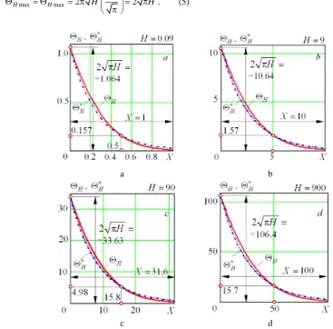
The dependences of the change in the dimensionless temperature over the depth of the subsurface layer, in-cluding the surface at X =0 for Н =0.09 (Fig. 3, a),
Н =9 (Figure 3 b), Н =90 (Figure 3 c) and Н =900 (Figure 3 d) are studied.
Data in Figure 3 allows estimating practical change in-tervals of dimensionless variablesH ,X and X/(2H1/2), which, first, correspond to a change range of regime pa-rameters for conventional operations of flat, round and profile grinding, and secondly, at which there is a dimen-sionless temperature field at the heating stage (Table 1).
It can be seen (Figure 3) that the error of the simplified equation (3) compared to the original equation (1) in the zone of a ten-fold temperature drop is alternating (first lowering the temperature, then its overestimation) and the lowest errors occur at high and medium temperatures. This is just in the region of significant temperature values that affect the nature and depth of the defective layer during grinding.
a b
c d
Journal of Engineering Sciences, Volume 6, Issue 2 (2019), pp. A 1–A 7 A 5 Table 1 – Formal and real intervals of changing the
dimension-less parameters at the heating stage at the heating stage
Formal interval Real interval
0 X 41.7 0 X 14
0.047H 104.063 4H 20 0
2
X
H
96 0
2
X
H
1
3.3 Comparing the models
To estimate the errors of the simplified dependencies (3) and (4) obtained, it is necessary to compare them with the similar more exact dependencies (1) and (2) at the heating and cooling time intervals, which were choose the same. Expressed through a dimensionless parameter H
(Peclet number), the interval of dimensionless heating time for a wide range of grinding modes is 0H 100.
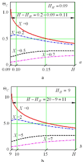
The study will be carried out, for example, in the most unfavorable case with H =0.09, since for H =4 the coincidence of the two-dimensional solution with the one-dimensional solution by equations (1) and (2) is most pronounced [11–14]. As an example in Figure 4 shows graphs of the change in the dimensionless grinding tem-perature at H =0.09, constructed from equation (2), that is, in the cooling stage.
Figure 4 – The change in the dimensionless grinding tempera-ture = С С( ,X H H, H)according to equation (21) at the cooling stage depending on the Peclet number H at fixed distances from the surface X at HH = 0.09 in the intervals
0H5(a) and 0H1 (b)
It can be seen in Figure 4 that a change ofHH from H
H =9 to HH =0.09 (a hundred times) leads to an in-crease in the scale of the dimensionless cooling time by ten times, i. e. just as it was noted in Figure 5.
a
b
Figure 5 – The change in the dimensionless temperature de-pending on the Peclet number H at the cooling stage (without
cooling liquid) at fixed distances from the surface X at H
H =0.09 (a) and HH =9 (b)
Comparison of the data on the grinding temperature change by equations (2) and (4) is shown graphically in Figure 5. It can be seen that, as at the heating stage, equa-tions (2) and (4) are close and have two points of coinci-dence: at 0 (i.e. on the surface) and at the depth of ap-proximately threefold decrease in temperature. You can also see that the nature of the ratio between the scales of change of the HH (0.09 and 9) and the X (1 and 10) is of 100 (9/0.09) to 10 (10/1).
A 6 MANUFACTURING ENGINEERING: Machines and Tools a
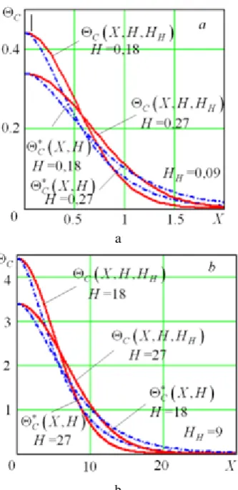
b
Figure 6 – The change in dimensionless temperature depending on the dimensionless depth Х in the cooling stage (without a cooling liquid) for HH =0.09 at H = 0.18 and H = 0.27 (a),
and for HH =9 at H = 18 and H = 27 (b)
The areas of use of the approximate expressions (3) and (4) are determined by comparing them with the cor-responding more exact expressions (1) and (2). To do this, we limit the allowable amount of error between the compared expressions, for example, by the levels
Н
= 11 % at the heating stage and C= 15 % at the cooling stage (Table 2).
Table 2 – Allowable intervals for changing the dimensionless parametersХ and Н
Н Heating stage Cooling stage 0.09 0Х 0, 6 0Х 1
20 0 Х 8, 5 0Х 15
100 0 Х 19, 5 0Х 33
The data given in Table 2 do not contradict the previ-ously found area of their change (see Table 1). It can be seen in Table 1 that the obtained expressions (3) and (4) can be used in fairly wide intervals of Х and Н varia-tion to estimate the grinding temperature and its distribu-tion over the depth of the surface layer.
4
Conclusions
Temperatures Hand Has well as the depth Х of the fixed temperature penetration, under otherwise equal conditions, are proportional to the square root of the Pe-clet number. The coordinates of the same point of the previous (i-1)-th solutions
(
Xi−1,Hi−1)
and(
Xi 1,Hi 1)
− −
with the subsequent i-th solutions
(
Xi−1,Hi−1)
and
(
Xi−1,Hi−1)
are the same and differ in the Hi/Hi−1 times. For example, when goingfrom Нi−1=0.09 to Нi=9, the coordinate of the coinci-dence points on the ordinate axis changes from 1.064 to 10.64, and on the abscissa axis - from 0.5 to 5.0, i. e.
1
/ 9 / 0, 09 10
i i
H H− = = times.
A study of the developed grinding temperature math-ematical model made it possible to establish its continuity with the existing solution of the one-dimensional differ-ential equation of heat conduction under boundary condi-tions of the second kind on the surface. At the same time, the developed new mathematical model, in contrast to the mentioned one-dimensional solution, makes it possible to explicitly determine the penetration depth of any previ-ously set grinding temperature.
References
1. King, R. I., Hahn, R. S. (1986). Handbook of Modern Grinding Technology. Chapman and Hall, New York, London. 2. DeVries, W. R. (1991). Analysis of Material Removal. Springer-Verlag, New York.
3. Isii, T., Simoyama, I., Inoue, H., et al. (1988). Mechatronics. The Piece, Moscow.
4. Lima, P. U., Saridis, G. N. (1996). Design of Intelligent Control Systems Based on Hierarchical Stochastic Automata. World Scientific Publishing Co Pre Ltd., Singapore.
5. Ross, A. (2016). The Industries of the Future. New York, Simon & Schuster Inc.
6. Carslaw, H. S., Jaeger, J. C. (1959). Conduction of Heat in Solids. 2nd edition. Oxford University Press, Oxford.
7. Jaeger, J. C. (1942). Moving sources of heat and temperature at sliding contacts. Proceedings of the Royal Society, Vol. 76, рр. 203–224.
Journal of Engineering Sciences, Volume 6, Issue 2 (2019), pp. A 1–A 7 A 7 9. Akbari, M., Sinton, D., Bahrami, M. (2011). Geometrical effects on the temperature distribution in a half-space due to a moving
heat source. Journal of Heat Transfer, Vol. 133(6), pp. 064502-1–064502-10.
10. Sipaylov, V. A. (1978). Thermal Processes during Grinding and Surface Quality Control. Mashinostroenie, Moscow.
11. Lishchenko, N., Larshin, V. (2020). Temperature field analysis in grinding. Advances in Design, Simulation and Manufacturing II, DSMIE 2019,Lecture Notes in Mechanical Engineering, Springer, рр. 199–208. Springer, Cham.
12. Larshin, V., Lishchenko, N. (2019). Adaptive profile gear grinding boosts productivity of this operation on the CNC machine tools. Advances in Design, Simulation and Manufacturing, DSMIE 2018,Lecture Notes in Mechanical Engineering, Springer, pp. 79–88.
13. Larshin, V. P., Kovalchuk, E. N., Yakimov, A. V. (1986). Application of solutions of thermophysical problems to the calcula-tion of the temperature and depth of the defective layer during grinding. Interuniversity Collection of Scientific Works, pp. 9–16. 14. Lishchenko, N. V. (2018). Profile Grinding Productivity Increasing on CNC Machines on the Basis of Grinding System
Elements Adaptation. D.Sc. thesis, 05.02.08 – Manufacturing Engineering. National Technical University “Kharkiv Polytechnic Institute”, Kharkiv.
УДК 621.923.1
Дослідження спрощеної моделі температури шліфування
Ліщенко Н. В.1*, Ларшин В. П.2, Крачунов Х.3
1 Одеська національна академія харчових технологій, вул. Канатна, 112, 65039, м. Одеса, Україна; 2 Одеський національний політехнічний університет, просп. Шевченка, 1, 65044, м. Одеса, Україна;
3 Технічний Університет м. Варна, вул. Студентська, 1, 9010, м. Варна, Болгарія
Анотація. У роботі проведене дослідження спрощеної математичної моделі визначення температури шлі-фування. За отриманими рівняннями цієї моделі є відмінність результатів від відповідного більш точного розв’язання одновимірного диференціального рівняння теплопровідності за граничних умов другого роду. Досліджувана модель представлена системою з двох рівнянь, що описують температуру шліфування на ета-пах нагрівання і охолодження без використання примусового охолодження. Обсяг досліджуваної моделі від-повідає сучасним технологічним операціям шліфування на верстатах із ЧПК для умов, коли числове значення числа Пекле перевищує 4. Це, у свою чергу, відповідає критерію Егера для так званого джерела тепла, яке швидко рухається, для якого параметр швидкості заготовки може бути еквівалентно за температурою заміне-ний часом дії джерела тепла. Це дає можливість використовувати більш простий розв’язок одновимірного диференціального рівняння теплопровідності при граничних умовах другого роду (одновимірна аналітична модель) замість аналогічного двовимірного розв’язку з невеликим відхиленням результатів розрахунку тем-ператури шліфування. Встановлено, що запропонований спрощений математичний вираз для визначення температури шліфування відрізняється від більш точного одновимірного аналітичного розв’язку не більше ніж на 11 % і 15 % на етапах нагрівання та охолодження відповідно. Порівняння даних щодо зміни темпера-тури шліфування за звичайним і розробленим рівняннями показало, що ці рівняння близькі та мають дві точ-ки збігу: на поверхні та на глибині (приблизно зниження температури втричі). Також встановлено, що харак-тер співвідношення між масштабами зміни числа Пекле (0,09 та 9) та глибиною температури подрібнення (1 та 10) становить 100 (9/0,09) і 10 (10/1) відповідно. Крім того, розкрито ще один нетрадиційний механізм для обох порівняних рівнянь: більш висока температура на поверхні супроводжується нижчою температурою на глибині.