Limits and Tradeoffs in the Control of Autocatalytic Systems

CONTROL OF AUTOCATALYTIC

SYSTEMS

Thesis by Fiona Chandra

In Partial Fulfillment of the Requirements for the degree of

Doctor of Philosophy in Bioengineering

CALIFORNIA INSTITUTE OF TECHNOLOGY Pasadena, California

2013

ACKNOWLEDGEMENTS

ABSTRACT

Despite the complexity of biological networks, we find that certain common architectures govern network structures. These architectures impose fundamental constraints on system performance and create tradeoffs that the system must balance in the face of uncertainty in the environment. This means that while a system may be optimized for a specific function through evolution, the optimal achievable state must follow these constraints. One such constraining architecture is autocatalysis, as seen in many biological networks including glycolysis and ribosomal protein synthesis. Using a minimal model, we show that ATP autocatalysis in glycolysis imposes stability and performance constraints and that the experimentally well-studied glycolytic oscillations are in fact a consequence of a tradeoff between error minimization and stability. We also show that additional complexity in the network results in increased robustness. Ribosome synthesis is also autocatalytic where ribosomes must be used to make more ribosomal proteins. When ribosomes have higher protein content, the autocatalysis is increased. We show that this autocatalysis destabilizes the system, slows down response, and also constrains the system’s performance. On a larger scale,

TABLE OF CONTENTS

Acknowledgements ... iii

Abstract ... iv

Table of Contents ... v

List of Illustrations and/or Tables ... vi

Chapter I: Introduction ... 1

Chapter II: Minimal Model of Glycolytic Oscillations: Limits and Tradeoffs ... 4

Minimal Model ... 4

Steady State Limits ... 7

Hard Limits on Robust Efficiency ... 11

Complexity and Robustness ... 16

Experiments in Single Cells ... 21

Chapter III: Single Cell Oscillations and Redox ... 28

Oscillations in Single Yeast Cells ... 28

Analysis of the Kloster Model ... 29

Redox Balance in Anaerobic S. cerevisiae ... 31

Glycolysis Model with Redox and Diffusion ... 32

The Role of Glycerol Production ... 40

Chapter IV: Ribosome Autocatalysis ... 43

Minimal Model of Ribosome Synthesis ... 44

Higher Order Model of Ribosome Synthesis ... 47

Tradeoffs in Ribosome Synthesis: Maximal Growth and Efficiency ... 49

Tradeoffs in Ribosome Synthesis: Feedback and Stability ... 49

Ribosome Synthesis During Starvation ... 51

Three-State Model of Ribosome Autocatalysis ... 53

Mitochondrial Ribosomes ... 63

Ribosome Heterogeneity ... 64

Chapter V: Evolution of Network Architecture ... 66

Power Law Distributions and Scale Free-ness ... 66

Transcription Network Architectures in Bacteria vs Yeast ... 67

Comparison of Generating Models ... 71

A Biologically Relevant Combined Model ... 73

Prokaryotic vs Eukaryotic Regulation ... 76

Chapter VI: Conclusions ... 78

LIST OF ILLUSTRATIONS AND/OR TABLES

Figure Number Page

2.1 Diagram of the two-state glycolysis model ... 7

2.2 The equilibrium point(s) of the system ... 9

2.3 Tradeoffs between waste, fragility, and complexity ... 10

2.4

Effects of higher autocatalytic stoichiometry

q

2.5 Log Sensitivity and step response of glycolysis without PK feedback ... 17

2.6 Log Sensitivity and step response a) with PK feedback b) with varying k .... 19

2.7 Histogram of glycolytic enzyme in cells grown in glucose vs ethanol ... 22

2.8 NADH autofluorescence in single cells grown in ethanol ... 25

2.9 NADH autofluorescence in single cells grown in glucose ... 25

2.10 Simulation of two state model recapitulating cell extract studies ... 27

3.1 Linear stability regions of Kloster et al’s model ... 31

3.2 Glycolysis models incorporating redox and diffusion ... 35

3.3 Stability regions of 7-dimensional glycolysis model ... 36

3.4 Stability regions of the 4-state glycolysis model ... 37

3.5 Extracellular acetaldehyde concentration ... 38

3.6 Stability analysis for varying NAD+ autocatalytic stoichiometry ... 39

3.7 Stability regions for varying number of NAD+ molecules and produced ... 39

3.8 Stability changes with the interaction of the two autocatalytic loops ... 40

3.9 Higher glycerol production rate is stabilizing ... 41

4.1 Growth rate for varying ribosome production ratio ... 46

4.2 Diagram of the 6-state ribosome synthesis model ... 47

4.3 Optimal ratio for growth and proportion of ribosomes in the cell ... 48

4.4 Stability regions mRNA production rates are varied ... 50

4.5 Simulation of the 6-state ribosome model ... 51

4.6 Sensitivity of steady state levels to various parameter perturbations ... 52

4.7 Optimal ratio for highest protein level in starvation condition... 53

4.8 Simulation of the 6-state ribosome model to sudden nutrient availability ... 54

4.9 Optimal riboprotein transcription ratioincreases with nutrient level ... 55

4.11 Cost of cell growth ... 57

4.12 Higher autocatalysis slows down response time ... 57

4.13 Minimum stable ratio as rRNA level increases ... …58

4.14 Optimal and minimum stable ratio as feedback strength increases ... …59

4.15 Optimal and minimum stable ratio as autocatalysis increases ... …59

4.16 Poles of 3-state ribosome model with varying rm and autocatalysis ... …61

4.17 Zeros of 3-state ribosome model with feedback from ribosomal protein to translation…61 4.18 Zeros of 3-state ribosome model with feedback from ribosomes to rRNA…62 4.19 At lower rRNA level, the system requires lower autocatalysis to maintain stability…65 5.1 Rank-degree plot of transcriptional regulatory networks ... 68

5.2 In-degree plot of transcriptional regulatory networks ... 68

5.3 Rank-degree plot of the operon-operon regulatory network in E. coli ... 70

5.4 The clustering coefficients of all three organisms ... 70

5.5 Clustering coefficients of the network generated by Yule process ... 72

5.6 Degree distributions of networks generated by Yule process and duplication divergence ... …74

5.7 A small power-law network is expanded via the duplication divergence mechanism …75 5.8 Distribution of network simulated with combined network model mimic E. coli network ... …76

5.9 Clustering coefficients of the network generated by combined model ... 76

Table Number Page 1. Parameters and definition of terms of the glycolysis model... 5

2. Tradeoffs in glycolysis with respect to various parameters... 21

3. Fluorescence statistics of GFP-tagged glycolytic enzymes ... 22

4. Parameter definitions of the 6-state ribosome model ... 48

5. Statistics of the three transcription networks ... 69

Equation Section (Next)

Chapter 1

INTRODUCTION

Minimizing waste, resource use, and fragility to perturbations in system components, operation, and environment (1) is crucial to sustainability of systems ranging from cells to engineering infrastructure. Much of the studies of the evolutionary basis of biological networks have been based on the idea that the networks optimize growth rate, but both engineering and biology are constrained by tradeoffs between efficiency and robustness which are rarely formalized in biology. Tools that are commonly used in optimization as well as in systems and control theory can provide a good foundation in understanding these tradeoffs in biological networks.

Certain network architectures have aggravated constraints and tradeoffs (2). One such architecture is autocatalysis, where a species is consumed in catalyzing its own production. This type of structure can grow uncontrollably without feedback regulation, yet we find autocatalysis in many crucial functions of the cell, including metabolism (glycolysis) and protein synthesis. Some autocatalysis is unavoidable due to the reaction energetics requirements as in the case of glycolysis. Glycolysis is a central energy producer in a living cell, consuming glucose to generate Adenosine Triphosphate (ATP) which is used throughout the cell. The first steps of the reaction require ATP, making it autocatalytic. The energy input from ATP hydrolysis is necessary to power thermodynamically unfavorable reactions.

glycolysis as a first case study, as it not only has interesting dynamics (e.g. oscillations) but has a rich literature experimentally and theoretically (3). Despite extensive experimental and modeling studies since 1965 (4), whether the oscillations are beneficial or simply an evolutionary accident remained unsolved. Using control theoretic analysis on a simple model, we suggest a third alternative: Oscillations are the inevitable consequence of tradeoffs between metabolic overhead and robustness to disturbances, as well as the interplay between feedback control and necessary autocatalysis of network products (5, 6). Our model is now also the simplest (with only two states) example of a system with a right-half plane zero and can be used as a tool for teaching some fundamental concepts of control theory.

C h a p t e r 2

MINIMAL MODEL OF GLYCOLYTIC OSCILLATIONS: LIMITS AND TRADEOFFS

Glycolytic oscillation, in which the concentrations of metabolites fluctuate, has been a classic case for both theoretical and experimental study in control and dynamical systems since the 1960s (12). Numerous mathematical models have been developed, from minimal models (4, 13) to those with extensive mechanistic detail (14). Besides being the most studied control system and the most common, glycolysis is also conserved from bacteria to human, and presumably has been under intense evolutionary pressure for robust efficiency. Thus new insights are less likely to be confounded by either gaps in the literature or evolutionary accidents compared with less well studied biological circuitry. Nevertheless, the function of the oscillations, if any, remains a mystery and one we aim to resolve.

The first step is development of the simplest possible model of glycolysis that illustrates the tradeoffs caused by autocatalysis. Biologically motivated minimal models of glycolytic oscillations exist, but analysis of robustness and efficiency tradeoffs has not received much attention. Such analysis can provide a much deeper understanding of the underlying basis of glycolytic oscillations, as well as illustrate universal laws that are broadly applicable.

Minimal Model

2 2

2 2

2 2

2 2

1 1 0

1 1 2 2

1 1

2 2

( 1) (1 )

( 1) (1 )

1 1

a

h g a

h g

a

h g

y kx

x

y y y kx

y y

y kx

q q

y q q

y y

PFK PK Consumption





Model Parameters Definition of Terms

x lumped variable of intermediate metabolites

P(s) Open loop response (h=0) in frequency (s) domain

y output, ATP level

k intermediate reaction rate WS(s) Weighted response to a disturbance



WS(s)=W(s)S(s) where W(s) is the weight



q autocatalytic stoichiometry S(s) Impulse response to a disturbance



a cooperativity of ATP binding to PFK z Zero, the solution to P(z)=0

h feedback strength of ATP on PFK p Pole, the solution to W(p)=P(p)=∞, or D(p)=0

g feedback strength of ATP on PK

Table 1.

normalizations). Our results hold for more general systems as discussed below and in SI, but the analysis is less transparent.

Like most research, we focus on allosteric activation of the enzyme PFK by Adenosine Monophosphate (AMP) as the main control point of glycolysis. We assume total concentration of adenosine phosphates in the cell [Atot]=[ATP]+[ADP]+[AMP] remains constant and the activating effects of AMP can be modeled as ATP inhibition. ATP also inhibits PK activity, although this has been largely ignored in most models (except (15, 16)). We emphasize its importance and model both inhibitions through exponents h and g.

We use linearization to focus initially on steady state error and instability while highlighting disturbance and control:

1

0

(

1)

(

1)

1

Disturbance Control

x

k

a

g

x

h y

y

q

k

qa

g q

y



q

 

       

 

       

 

      























 







Figure 2.1. (A) Diagram of two state glycolysis model. ATP along with constant glucose input produce a pool of intermediate metabolites (phosphorylated six-carbon sugars), which then produces two ATPs. ATP inhibits both the first (Phosphofructokinase/PFK-like) and second (Pyruvate Kinase/PK-like) reactions. (B) Control-theoretic diagram of the same system (arrows represent logical connections, not fluxes.) The system without inhibition/feedback is labeled the “Plant” (P; solid box, solid and dotted loop in (A)) while the inhibitory mechanism is considered the “Controller” (here labeled by its inhibitory strength, H; dashed loop in (A) and (B).) The effect of disturbance



Steady State Limits

The simplest robust performance requirement (motivated by the need to maintain high energy charge) is that the concentration of y remain nearly constant despite fluctuating demand . In our

model this requires that the steady state error ratio, obtained by solving for y





when

0

0

x

y

           







1 y

h a



 _

 (2.3)

more costly for the cell to produce. A more interesting tradeoff arises because (2.2) is stable if and only if





0 h a k g q q

 

   _(2.4)

The left boundary indicates where the system is unstable (unstable node) while the right boundary indicates where the system starts to oscillate (limit cycle).

We can plot f(y) vs. y and the equilibrium points are the intersections of f(y) and the consumption rate of ATP, which in this model is normalized to 1 (Figure 2.2). There is one equilibrium point when a2h (Fig 2.2A and B) and two when a2h(Fig 2.2C and D). We can show using linear stability analysis that when the (1, 1/k) equilibrium point is either stable or in a limit cycle, the other equilibrium point is always unstable, with one positive and one negative eigenvalue (a saddle node). In fact, we can show that the equilibrium point is unstable when the slope of f(y) is positive and thus the lower equilibrium point is unstable. If we relax the normalization for ATP consumption then the equilibrium point moves with the consumption. A study by Kloster and Olsen also confirms that the activity of intracellular ATPase significantly affects oscillations (17).





1

1

y

q

h a

k

g

q















Figure 2.2. The equilibrium point(s) of the system is given by the intersection(s) of the curve f(y)

(blue) with 1 (red).A) a=h=1. B) a =1 < h=2. C) a=1 < h=8. D) a=5 < h=8.

Equation (2.5) and Fig 2.3A (showing the error bound (2.5) versus k) illustrate a simple and elegant tradeoff between robustness and efficiency (as measured by complexity and metabolic overhead). Low error requires large h, but to allow this to be stable, k and/or g must also be large enough. Large k requires either more efficient or higher level of enzymes, and large g requires a more complex allosterically controlled PK enzyme; both would increase the cell’s metabolic load. Thus fragility directly trades off against complexity and high metabolic overhead (low efficiency).

Thus at least in this model, oscillations have no direct purpose but are side effects of hard tradeoffs crucial to the functioning of the cell, and can be avoided at some expense. Note that robustness means making fragility (steady state error and oscillations) small, and efficiency means making metabolic overhead (enzyme amount and complexity) small.

Figure 2.3. Tradeoffs between waste, fragility, and complexity due to enzyme complexity and amount. Enzyme amount affects the intermediate reaction rate k (x-axis), plottedfor g=0 (solid) and

Hard limits on robust efficiency

Thus far we described simple tradeoffs based on basic biochemical features of a minimal model. Our elementary analysis of (2.2) is consistent with existing literature, yet clarifies in (2.5) how oscillations are the inevitable side effect of robust efficiency and tradeoffs between steady state error and stability. An important next step is to expand to a more detailed and comprehensive model, and also extend the analysis to study global nonlinear stability, stochastics, and worst-case disturbances. We have explored such dimensions and the results are consistent, though often less accessible (most additional modeling details make the tradeoffs worse).

A more fundamental direction, however, is to rigorously prove that the tradeoffs suggested by (2.5) are unavoidable regardless of these neglected details, depend only on the basic properties of autocatalytic and control feedbacks, and are unlikely to be either artifacts of model simplifications or “frozen accidents” of evolution (of course, in principle anything is possible since there is always some gap between models and reality.) Fortunately, control theory has been developed precisely to address such questions in engineering. Unfortunately, while well known to engineers and mathematicians, control theory has not been integrated into other fields. A good background is given in (3).

written using frequency-domain transforms

y s

ˆ

 

y t e dt

( )

  



, where s is the (complex)

Laplace transform variable, and frequency



s



j



The weighted sensitivity transfer function defined as

WS s

 

y s

ˆ

   

/



ˆ

s

to y. Given (2.2) and controller H, we can factor WS s

 

   

WS can be calculated as follows:





( )

(

)

( )

(

)

0

0 1

(

1)

(

) (

1)

1

(

(

))

(

)

Y s

WS

C sI

A

B

D s

s

k

a h

g

q

k

s

q a h

q

g

s

k

s

k

g

q a h

g s k a h

 







  



  





  

 



  

 









  

 





(2.6)

Which can be separated into the Weight W and Sensitivity function S:

2

2 2

( )

( ) ( )

(

(

))

(

(

))

(

(

))

(

)

WS s

W s S s

s

k

s

k

g

q a

g s ka

s

k

g

q a

g s ka s

k

g

q a h

g s k a h









  











  







  

 







(2.7)

Therefore, disturbance , W(s), S(s) and the open loop response P(s) are given by:

 

1

( )





( )

( )

( )

1

( )

( )

( )

( )

( )

s

k

D s

qs

k

W s

S s

P s

D s

P s H s

D s

H s

qs

k

D s



 







where

 

( ( ))

D s s  k g q ag ska. With constant, stabilizing H(s)=h>a, it follows from (2.8) and (2.5) that the response at frequency =0 is equal to the steady state error ratio:

 

   

1

1





0

0

0

1

y

a

q

WS

W

S

a h a

h a

k

g

q























S is the primary robustness measure for feedback control (2), and |S(s=j)| measures how much a disturbance is attenuated (|S(j)|<1) or amplified (|S(j)|>1) at frequency .

S s

( ) 1



 

H s  . The response of y to any other disturbance can be treated with the appropriate weight

W.

When there is autocatalysis, we can derive stricter bounds on the response WS and S, using the maximum modulus theorem from complex analysis. In (2.8), when q>0, P(s) has a zero at z=k/q

defined as P(z)=0 which is positive real (Re

 

 

 

 

 

 

   

Re 0

max

max

j s

q

WS

WS j

WS s

W z S z

k

qg















 

max

j

s

p

z

p

S

S j

S

s

p

z

p

















The norm WS _ has a variety of interpretations (2), the simplest of which is the maximum sinusoidal steady state response for any frequency . Ideally, both WS and S should be low at all frequencies, but this contradicts (2.10) and (2.11), which hold regardless of the controller used.The peak WS _is always larger than the bound in (2.10) for any h, and that minimizing steady state error |WS(0)| leads to WS _∞ and oscillations. Fig 3B shows how the RHS of (2.11) varies with

k and g; both (2.10) and (2.11) are aggravated by small k and g. These are hard constraints on any stabilizing controller from y to the first enzyme, no matter how complex the implementation, and thus are much deeper than (2.5) which applies only for constant H=h.

Conditions such as (2.10)-(2.11) can be applied to other transfer functions and weights to provide a rich theoretical framework for exploring additional tradeoffs and details, including realistic frequency content of (t), appropriate error penalties in y(t) and other signals, and other sources of noise and uncertainty (2, 21). A complementary focus is on constraints that are independent of these details, such as Bode’s Integral Formula (2):

 

0

1

ln S j

 









that holds for any linear, stabilizing H that is causal (i.e. H cannot depend on future values of y(t).

H=h depends only on current values.) This “water bed” effect implies that the net disturbance attenuation (ln|S(j)|<0) is at least equaled by the net amplification (ln|S(j)|>0). It is a general constraint on WS s

 

 

   

 

 

lnWS j











tune the shape of ln S j

 

 

1

lnS j z d max 0, ln z p

z z p

     _{  }  _{ }  _  _



when z,p>0 . (2.13) is a variation of the Bode Integral Formula and we can prove that this holds for relative degree <2 as follows:

We start with the following lemma (see Chapter 6 of (2) for proof):

Lemma 1:

Let S be analytic and of bounded magnitude in Res≥0 and let: z 









0

2 2

0

1

( ) ( )

( )

S z S j











 

 



 



We can factor S as:

ap mp

S



S S

Sap is defined as the product of all factors of the form

s

p

s

p





poles (where S(p)=0) and _mp ap S S

S

 . Since S(z)=1, ( ) 1 ( ) mp ap S z S z 

Lemma 2 : For every point z 









0

2 2

0

1

ln | ( ) | ln | ( ) |

( )

mp

z

S z S j d

Then for our two state model with one z>0 and one p>0 we can write:

2 2

1

ln | (

S j

) |

z

d

ln

S

( )

z

ln

z

p

z

z

p





















It is easily shown that p>0 when a>0, and otherwise (2.13) is just bounded by 0. Hence autocatalysis always causes positive z and p and the integral in (2.13) is bounded similar to (2.11).

The low pass filter ₂ z ₂

z  constrains the waterbed effect to below frequency =z. Small z=k/q produces a more severe limitation since any disturbance attenuation must be repaid with amplification within a more limited frequency range. Fig 2.3B shows the tradeoff in three criteria: high k both stabilizes the system and reduces the bound but implies high metabolic overhead. Fig 2.4B illustrates how autocatalysis and (2.13) impact dynamics.

Figure 2.4. Effects of higher autocatalytic stoichiometry q. Higher autocatalysis results in higher peak in the Sensitivity function, S (left) which corresponds to more ringiness in the transient response (right) and eventually leads to oscillation.

0 2 4 6 8 10

-1.2 -1 -0.8 -0.6 -0.4 -0.2 0 0.2 Time Time Simulation

0 2 4 6 8 10

S(0)gives the steady state error while the peak in S(j) corresponds to how “ringy” the transient y(t)dynamics are at frequency . At h=2, S(0) is large, the peak S _is low, and y(t)has a large steady state error, which h=3 lowers but with more transient fluctuations. At h=4 the system oscillates at the frequency where S(j)∞. Larger q makes z smaller and performance worse (more ringy), shown in Fig 2.4. The tradeoff in (2.5) and the difference between (2.12) and (2.13) disappears with no autocatalysis (q0) because the RHS bound in (2.5)∞, and in (2.13)0. Zero steady state error with stability is then possible by taking h∞.

Complexity and robustness

We have taken PFK feedback as the main controller, but the often neglected PK feedback increases enzyme complexity and plays an important but subtle role in robustness. Most simply, increasing g

uniformly improves the stability bound in (2.5). From (2.4), if q=a=1, then the system is stable for

Figure 2.5. Log sensitivity log|S(j)| (i) without ATP feedback on PK (g=0) and step response of the nonlinear system (2.1) to step change in demand (ii). The integral of log|S(j)| is constrained by (2.12) in A.i and (2.13) in B.i and is the same for all h.Only the shape changes with increasing h.

disturbances with those in (22) on robustness to internal noise in transcription.

From an engineering perspective, this is a remarkably clever control architecture, and the presence of g>0 suggests that at least in this case evolution favors higher complexity in exchange for flexibility in k and robustness. Further insights come from the bound in (2.13). Since z=k/q, increasing k improves both sides of (2.13) and uniformly improves robustness (Fig 2.6B), at the expense of higher enzyme levels. Increasing g decreases p while leaving z unchanged (

2

(

)

(

(

))

4

2

k

g

q a

g

k

g

q a

g

ka

p



  





 





z p



 (Fig 2.3B). This

improves the constraint in (2.13) and enables more aggressive controller gains h on PFK. By itself (when h<a) however, g>0 cannot stabilize, and a stabilizing G(s) would actually need to be an unstable controller which needs very high complexity (see SI-VI in (5)).

Our simple model thus far restricts the controller implementation to ATP inhibition, but other intermediate metabolites can also have inhibitory effects. We show that control by intermediate metabolites can relax stability and performance constraints at the cost of lower efficiency.

Glycolytic enzymes, and PFK in particular, have a complex regulatory control. PFK is known to be not only inhibited by ATP but also by its immediate product, fructose 1,6-bisphosphate (F1,6bP) (23). We look at the effect of allowing PFK inhibition by the intermediate, x (note that to maintain basal rate of PFK and steady state y concentration to 1, the net inhibition of x on PFK is normalized to be (kx)-f)

1 1 0

( ) (1 )

1 1

h f g

a

PFK PK Consumption

x d x

y y kx kxy

y dt y q q 

  

         

         

 

       



   

The steady state error ratio for this model is:

1

(

)

y

f

h a

fg









 

(2.19)

This new system has stability bounds: 0

( ) 0

h a fg

k kf g q a h g

  

     

(2.20)

which relaxes the stability constraints and further bounds the steady state error to be:













1 1

( ) 1

q f

y f

h a fg k q g f k gq





 _  _

     

(2.21)

The functions S and P are now given by:

2

2

( ( ))

( ( )) ( )

s k kf g q a g s ka kfg S

s k kf g q a h g s k a h kfg

      



        

(2.22)

2

( )

(

(

))

qs

k

P s

s

k

kf

g

q a

g s ka

kfg

 



 

 







(2.23)

And hence the

zero

remains the same as

z

k

q



.

Intermediate inhibition on PFK can thus change both the steady state error and stability bounds, while intermediate activation of PK can lift performance constraint (ultimately, the effects of both are limited by enzyme saturation). Fructose 1,6-bisphosphate (the product of PFK) has been thought to both inhibit PFK and activate PK, again suggesting that nature accepts greater complexity in return for robustness.

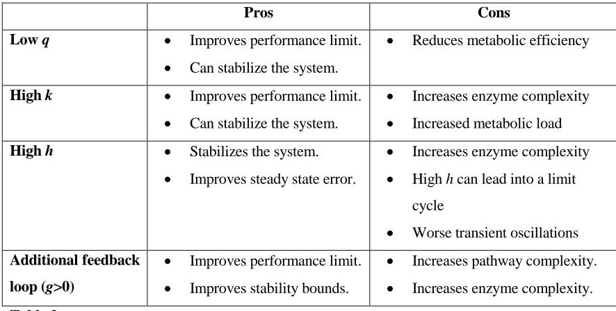
Pros Cons

Low q  Improves performance limit.

 Can stabilize the system.

 Reduces metabolic efficiency

High k  Improves performance limit.

 Can stabilize the system.

 Increases enzyme complexity

 Increased metabolic load High h  Stabilizes the system.

 Improves steady state error.

 Increases enzyme complexity

 High h can lead into a limit cycle

 Worse transient oscillations

Additional feedback

loop (g>0)

 Improves performance limit.

 Improves stability bounds.

 Increases pathway complexity.

 Increases enzyme complexity.

Table 2

Experiments in Single Cells

Our theory shows both how autocatalysis makes glycolysis more prone to sustained oscillations and how sufficiently complex feedback control ameliorates this potential fragility. The tradeoffs summarized in Table 2 suggest that ringy transient dynamics would be more likely under specific worst case conditions that we have attempted to create experimentally. Small z=k/q has the most obvious impact on overall fragility, and this occurs at high autocatalytic stoichiometry q and/or low

Transcription levels of some glycolytic genes are decreased when S. cerevisiae is grown in ethanol (24), which could decrease k. Flow cytometry of S. cerevisiae cells with GFP-tagged enzymes (from Invitrogen GFP library) indeed show a lower abundance of glycolytic enzymes involved in the intermediate reaction including Fructose 1,6-bisphosphate aldolase (FBA1) and Glyceraldehyde-3-phosphate dehydrogenase (TDH3) (Table 3). Flow cytometry data was analyzed using FlowJo.

FBA1 fluorescence (AU) TDH3 fluorescence (AU)

Mean Median Mean Median

Glucose 564.1 552.5 423.5 352.3

Ethanol 468.8 393.7 301.5 198.1

Table 3. Fluorescence statistics of GFP-tagged glycolytic enzymes in yeast cells grown in media with glucose vs ethanol.

Interestingly, the level of TDH3 also shows higher variability when grown in ethanol, as shown in Figure 2.7, further underlining the importance of robust stability for all k>0.

Figure 2.7. Fluorescence histogram of GFP-tagged

Wild type yeast S. cerevisiae cells (strain W303) were then grown overnight in Yeast Nitrogen Base (YNB) + ethanol. Cells were then imaged using the microfluidic platform ONIX (CellAsic) and an inverted microscope (Nikon Eclipse Ti-E). We imaged the NADH autofluorescence (excitation 370 nm, emission 460 nm) in the cells as the ethanol medium was switched to a medium containing YNB, glucose, and potassium cyanide (KCN) to induce anaerobic glycolysis. Both simultaneous and independent addition of glucose and KCN were performed. During the media shift, we chose the highest flow rate which would not dislodge the cells, in order to ensure the media was shifted as abruptly as possible. For the ONIX microfluidic pump, this flow rate was at 7 psi. In a separate experiment, cells were harvested and starved by resuspending them in phosphate buffer (PBS) before adding glucose and KCN, which induces oscillations in dense cell suspension (25). Control cells were grown in YPD and shifted to YNB, glucose, and KCN.

Fluorescence measurement was taken every 3 seconds. Photo bleaching occurred after approximately 15 minutes, hence we analyzed only the early time points (Fig 2.8 shows measurements during the first five minutes). Note that while synchronized and sustained oscillation is found in dense whole yeast cell suspension, we could not achieve this density on a single cell layer using the microfluidic chamber.

Concentrations of KCN and glucose were varied and responses were compared, but no sustained oscillation was observed. Further attempt to stress the cells by heat shock (which unfolds enzymes, lowering k, and increases ATP demand) or by amino acid starvation (lowering enzyme levels) still did not induce oscillations. The period is in good agreement with the 36s period in cell suspensions (25), and this transient does not occur in cells grown in glucose (Fig 2.9), also as expected for high k

(e.g k=5 in Fig 2.6B(ii)). We observed no sustained oscillation regardless of the experimental perturbations applied, suggesting that the intact single cell is indeed rather robust.

Figure 2.9. Single cell NADH autofluorescence measurements in yeast cells grown in glucose made anaerobic using potassium cyanide (KCN). Black line indicates when KCN was added. No fluctuation was observed in the transients and cells NADH fluorescence returned close to its original value.

there is much more to be done theoretically and experimentally to fully resolve this. Chapter 3 discusses the problem of single cell oscillations further.

Agreement with Yeast Extract Experiments in Continuous Stirred Tank Reactor

In a continuous stirred tank reactor (CSTR) experiment, we can assume that the mixture inside the tank reactor is well mixed and thus can be modeled essentially as a single cell. Both yeast extract and glucose were flown into the tank reactor at the same rate, and the mixture was flown out keeping the volume in the tank constant. Other researchers observed early on that the concentration of NADH in these extracts oscillate when the flow rate is varied (26). NADH is stable at low flow rate and starts to oscillate when the flow rate is increased. When the flow rate is increased even more, NADH returns to being stable. This is perhaps the most well-known experimental result in glycolytic oscillation and the oscillation in NADH is later shown to correspond to oscillation in other glycolytic intermediates.

Our model can be simply modified to capture this extract case. We model the flow rates as a “consumption” of the produced metabolites, characterized by the parameter v. The inflow of ATP from the extract is modeled by the parameter u and is half of the initial concentration of ATP that is added into the extract.

2 2

2 2

2 2

1 1

2 2

( 1)

1 1

a

x g h

a

x g h

k x Vy

x vx

y y

k x Vy

y u q q vy

y y

  

 

    

 

(2.24)

equilibrium. When the v is increased, the system at some point passes through a bifurcation and starts to oscillate. However, when v is increased even more, the system moves back to a stable region. The bifurcations occur when k is low (as predicted by our theory), which is the case in a dilute extract solution, but which is a condition intact cells have probably evolved to avoid or cannot survive in.

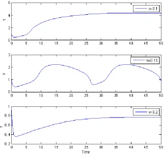
Figure 2.10. Simulation of our two state model (2.24) qualitatively recapitulates experimental observation from previous CSTR studies including (12, 26). As the flow of material in/out of the system is increased, the system enters a limit cycle and then stabilizes again. In this simulation, the parameters have been normalized so that the steady state concentration of ATP is 1. For this simulation, we take q=a=V=1, k=0.2, g=1, u=0.01, h=3.

C h a p t e r 3

SINGLE CELL OSCILLATIONS AND REDOX

Oscillations in Single Yeast Cells

The presence of oscillations at the population level in intact yeast cells seems to depend on high cell density, and the amplitude depends on the cell density. Until 2012, no oscillation was observed in sparse population of yeast cells, even when cyanide was added. As the density is increased, the entire population starts to oscillate in synchrony (27). There is some evidence that acetaldehyde, which diffuses in and out of the cells, is the synchronizing species (28, 29). Although some models, such as those by De Monte, capture this density dependence, De Monte explicitly models an oscillator instead of a mechanistic reaction model and thus does not explain why the density dependence occurs (30). Other models explore how acetaldehyde might synchronize oscillations between cells, but the long-standing controversy was how the cells behave at low density (31): do the single cells synchronize out of phase at low density, or are they stable and then start to oscillate synchronously as the density is increased? Lacking the technology, previous studies from each side of the argument have used indirect methods to answer the question.

through the chamber and the cyanide concentration were in a certain range. So far, this is the only paper that has reported oscillations in single isolated S. cerevisiae cells, although Weber et al reports that immobilized S. carlsbergensis cells desynchronize to out of phase single cell oscillations (33) (while they are both yeasts and the glycolytic pathway structure is universal, there are differences in the conditions required to achieve oscillations in the two organisms (34)). In our single cell studies, we kept the same cyanide concentration and chose the flow rate to be the maximum without dislodging the cells, and this may be beyond the oscillatory range.

Gustavvson et al suggested that the right concentration of extracellular acetaldehyde (low, but not too low) must be maintained for synchronized oscillations (32) and that this is achieved by the addition of potassium cyanide (KCN) to the medium. Cyanide not only halts aerobic metabolism but also reacts with the extracellular acetaldehyde which is released by the cells. Acetaldehyde reacts with NADH (to produce ethanol and NAD+) which is involved in the upper reactions of glycolysis and is coupled with ATP. Gustavsson et al showed that increasing flow rate through the microfluidic chamber can replace the role of cyanide in inducing oscillations (the cells must still be made anaerobic by flushing the medium with nitrogen). They observed heterogeneity in the responses where about 40% of the cells exhibit sustained oscillations and simulations of their detailed model captures this heterogeneity. However, they did not show one of the most important issues, which is whether the cells bifurcate from steady state to an oscillatory state as the flow rates (and thus acetaldehyde removal) are varied. It is still unclear whether their model captures this behavior.

species would be equivalent of increasing ATP consumption, which we have shown affects oscillations. The authors claim that they have explored a model where the autocatalytic and diffusing species are different (much like ATP and acetaldehyde) and that the results were consistent, but these results were not presented in the paper.

Analysis of the Kloster Model

In their paper, Kloster et al showed how the amplitude of the oscillation changes as the density is increased in their model (the amplitude is taken as zero when there is no oscillation). We looked at the stability of this model to see if it will also capture the effects of changing flow rate or cyanide concentration (essentially changing the rate of acetaldehyde removal from the external medium) in inducing oscillation.

The three-state model proposed by Kloster is as follows:

1

[ ]

([ ] [ ] ) ( , ) [ ]

([ ] [ ] ) 2 ( , ) [ ] [ ]

([ ] [ ] ) [ ] i

A e i

i

B e i B i

n e

B i e e e

i d A

D A A A B

dt d B

D B B A B k B

dt d B

D B B k B

dt n









  

   





(3.1)

Where [B]i and [B]e is the intracellular and extracellular concentration of species B, respectively.

The two variables to study here are the density n (and



Using the parameters given in (17), we performed linear stability analysis which indeed shows that there is a range of low density where the system can go from stable to an oscillatory state and back to stable as the diffusing species removal rate is increased (see Fig 3.1), as experimentally shown in (32). The experiment in (32) was performed at a particular low density (maintained using optical tweezers) which may lie in this range. Linear stability analysis indicates that if the density is decreased even more oscillations may not occur for any removal rate (given the parameters used in (17)).

Figure 3.1.

Linear stability of the Kloster model with density (



We then explored a more mechanistic model to see if similar behavior that corresponds to the single cell experiments can be achieved.

Redox Balance in Anaerobic S. cerevisiae

The glycolytic pathway produces two NADH, a reducing agent which is then used as an electron donor in the electron transport system to produce more ATP. However, in anaerobic conditions the electron transport system is shut down and NADH becomes a waste product. The NAD+/NADH ratio and the redox balance of the cell is very important and must be maintained, because many reactions depend on the proper NAD+/NADH ratio (typically this ratio is kept high in the cell). Thus, without the electron transport system, anaerobic cells must regain redox balance and high NAD+ level through another pathway. In S. cerevisiae, this is mainly achieved through glycerol and ethanol production, which oxidizes NADH into NAD+ (35). In fact, mutant cells that are unable to synthesize glycerol cannot grow anaerobically (36).

In addition to the NADH produced by glycolysis, some biosynthetic pathways also result in NADH production. In anaerobic S. cerevisiae, acetic acid is still produced, and further metabolized into acetyl-CoA, an imperative building block of fatty acid biosynthesis. The conversion of acetaldehyde into acetic acid produces 2 NADH.

TCA pathway activity is still maintained during fermentation to supply the amino acid biosynthetic precursors, but in a branched fashion. One branch forms 2-oxoglutarate and is oxidative while the other forms fumarate and is reductive; however, the reductive branch produces more NADH than is consumed by the oxidative branch, so it must still be compensated by either glycerol or ethanol production (35).

Glycolysis Model with Redox and Diffusion

The minimal model in Chapter 2 does not incorporate any species diffusion out of the cell and is not able to capture the density dependence of intact cell oscillations. This model was expanded to include acetaldehyde with diffusion and its reaction with NAD+/NADH. We developed two models to explore the role of cell density and media flow rate. The first model has seven states incorporating the previous ATP autocatalytic loop, NAD+ autocatalytic loop and acetaldehyde diffusion in and out of the cell (Fig 3.2A).

1 1 2 3 2 2 3 2 3 2 2 2 2

(

1)

2

1

2

1

2

1

(

)

2

1

2

1

eth out in e

g

e out in e cyan e

eth glyc N

a

h

a

h

A

X

k X

Y

q

k X

k YN

k

Y

k Z

Z

k YN

A

k Z

A

A

q

A

k Z

C

k C

k C

k C

A

C

k C

k C

k

C

N

k C

k

Y

k YN

V

A

V

A





























































(3.2)

X, Y, and Z are lumped intermediate metabolites, A represents ATP, N represents NAD+, and C and

(the NAD+ production step is actually the production of glycerol-3-phosphate, a precursor to glycerol). There is a consumption of N (NAD+), equivalent to production of NADH from the biosynthetic pathways, as dictated by the demand of the cell for biosynthetic building blocks. The consumption is assumed to be a constant determined by the growth requirements of the cell. In this model, kin=koutas they are diffusion parameters.

We asked if the expanded model could capture the experimentally observed behavior in (32). The key behaviors we looked for was: 1) the system goes from stable to a limit cycle as density increases, and 2) for lower density, the system can go from stable to a limit cycle and back to a stable region as the acetaldehyde removal rate is increased (either through increasing cyanide concentration or flow rate).

A B

Figure 3.2. A) 7-dimensional model of glycolysis and acetaldehyde diffusion. B) 4-dimensional model of glycolysis and acetaldehyde diffusion. There is an autocatalytic loop of ATP, which also inhibits PFK and PK. An intermediate metabolite is converted into glycerol in a reaction that produces NAD+. NAD+ is used as a substrate in an upstream reaction. One of the end products, acetaldehyde, diffuses in and out of the cell and is removed by cyanide in the media. Intracellular acetaldehyde is converted into ethanol in a reaction that also produces NAD+, completing the autocatalytic loop.

Figure 3.3. Stability of the 7-state model. The area in red shows the parameter region where the system is oscillating, while the area in white is where the system is stable. Just like in the Kloster model, the system goes into limit cycle as density is increased. At lower density the system moves from stable to oscillating to stable as the acetaldehyde removal rate is increased. 2 2 2 2 2

2

1

(1

)2

1

2

(

)

1

(

)

2

1

2

1

prod cons g g out in e c

e out in e cyan e

a

h

a

h

A

kXC

X

k X

A

q kXC

A

A

q

A

kXC

C

m

m

k X

k C

k C

d

A

C

k C

k C

k

C

V

A

V

A















































(3.3)

In this model, since NAD+ is lumped with acetaldehyde, kin encapsulates both the diffusion and the ethanol reaction, therefore

k



k

( ) 0

(1 ) ( ( ) ( 1) ) (1 ) 0

( ) ( ) ( ) 0 0 e e g ss ss ss

prod cons ss g prod cons out prod cons ss in

out in cyan

X X A A A C C C C

kC k V a h g kX

q kC V q a h q g q kX

A

m m kC k g m m V k m m kX k

k k k

           _                         _{     }               _{ }     

(3.4)

Where Xss and Css are the steady state values of X and C, respectively.

First, we take

m



1

Figure 3.4. Stability regions of the 4-state glycolysis model with mcons=mprod=1. The red shows the limit cycle region while white is the stable region. The plot shows that the system goes from a stable state to a limit cycle as the density is increased. Additionally, at lower density the system can go from stable to limit cycle and back to a stable state with increasing acetaldehyde removal rate. Parameters used were a=1; h=3; g=1; q=1; V = 4.0136;k =6.0459; kg=0.5927; kin = 1.0492; kout = 3.1639;

kc=4.7862;

There is in fact no specific range of extracellular acetaldehyde concentration that pinpoints if the system would oscillate. That is, while there does seem to be a minimum required concentration of acetaldehyde to affect the glycolytic reactions and induce oscillations, the maximum concentration in the oscillatory region is actually higher than the maximum in the stable region, thus there is no range where the system always oscillates (Fig 3.5).

1 0

Density (alpha)

A

ce

ta

ld

e

h

yd

e

R

e

m

o

va

l

R

a

Figure 3.5.

Extracellular acetaldehyde concentration (Ce) spanning a range of densities and

acetaldehyde removal rates. The left shows the concentrations found in a stable parameter set (black) while the right shows concentrations for parameter sets where the system oscillate. The system does not oscillate when [Ce] is too low but there is no

range of extracellular concentration that determines if the system will always oscillate.

This result can be easily tested experimentally by adding a flow of acetaldehyde to the extracellular medium of cells and checking if varying this concentration will change the cellular behavior (most studies have tried adding pulses of acetaldehyde, which only changes the concentration transiently (29, 37)). In (27) it is shown that the addition of acetaldehyde did not abolish oscillations, which supports our results above, but the acetaldehyde concentration added needs to be systematically varied.

Figure 3.6. Linear stability analysis for varying NAD+ autocatalytic stoichiometry vs. density (left) or acetaldehyde removal rate (right). The system is stable when the net NAD+ production is 0 (mprod-mcons=0) regardless of acetaldehyde removal rate. The system is also most robust in the switching behavior as density is increased at mprod-mcons=0.

Probing the parameter space further reveals that the behavior in the NAD+ autocatalysis results from its interaction with ATP autocatalysis. Figure 3.8 shows the stability as both NAD+ and ATP autocatalytic stoichiometry is varied. We see that for lower ATP autocatalysis q, lower NAD+ stoichiometry is indeed more stable.

Figure 3.8. How stability changes with the interaction of the two autocatalytic loops. NAD stoichiometry gives the net number of molecules produced (mprod -mcons), which is 0 in the real pathway. For q=0, lower NAD stoichiometry is stable but becomes unstable at higher q.Red is the oscillatory region and blue is the unstable region.

The Role of Glycerol Production

In glycolysis, the six-carbon sugar fructose-1,6-bisphosphate is cleaved into two three-carbon sugars, dihydroxyacetone phosphate (DHAP) and glyceraldehyde-3-phosphate (G3P), which can be interconverted by an isomerase. G3P goes on along the glycolytic pathway to eventually produce pyruvate and ATP, while DHAP is either converted into glycerol or converted back to G3P. As discussed above, in anaerobic conditions yeast cells ramp up glycerol production in order to oxidize NADH to NAD+ and maintain redox balance. Deleting the enzyme glyceraldehyde-3-phosphate dehydrogenase, which produces NAD+ along with glycerol-3-phosphate eliminates oscillations (38). It is also known that mutant cells which cannot synthesize glycerol cannot survive in anaerobic conditions.

When there is no glycerol production at all, or kg=0, the model (3.3) actually has no positive steady state. To see what role (other than maintaining redox balance) changing the rate of glycerol production has on the pathway, we also looked at the stability as glycerol production rate is increased. Fig 3.9 shows that increasing glycerol production rate allows stability for different

0 0.5 1 1.5 2 2.5 3

-3 -2 -1 0 1 2 3

ATP autocatalysis (q)

N

A

D

st

o

ich

io

m

e

tr

autocatalytic stoichiometry of both NAD+ and ATP. Plotting the stability regions of glycerol production rate kg vs. other parameters, including density and acetaldehyde removal rate showed that the system oscillates at low kg but is stable at higher kg, indicating that kg indeed confers stability. This is interesting, as our model does not impose redox balance constraints, yet increasing glycerol production not only helps maintain redox balance but apparently also stabilizes the system. Glycerol production branches off the glycolytic pathway and consumes DHAP, therefore increasing glycerol production decreases the downstream output (including ATP). This presents another tradeoff between robustness (stability) and efficiency (ATP output per glucose).

C h a p t e r 4

RIBOSOME AUTOCATALYSIS

Equation Section (Next)

Ribosome synthesis is another significant autocatalytic loop in a cell. Ribosomes are required to synthesize peptides and proteins, but are also partially composed of proteins themselves, thereby creating an autocatalytic loop. As we have seen in the previous chapters, autocatalysis can produce undesirable behavior, such as oscillation or fluctuation. Is there a similar consequence to autocatalysis in the case of ribosomes? Ribosome concentration is known to have low noise level (39). Changes in ribosome concentration can drastically affect the protein expression level even when mRNA levels are constant, and computational studies suggest that in some cases it may even lead to ultrasensivity (40). Fluctuations in the ribosome level therefore can lead to extremely noisy protein expression and can be detrimental to the cell.

This loop also presents the problem of resource allocation. Would the cell benefit more from allocating ribosomes to make more ribosomes, or to make other types of proteins? Is there an optimal ratio, and how is this ratio controlled? The cell devotes a significant amount of resources to ribosome production. Ribosomal mRNA transcription accounts for about 50% of the RNA Polynomerase Pol II transcription in yeast (41) while Pol I transcribes ribosomal RNA (rRNA) exclusively.

are not complexed with rRNA) inhibit ribosomal protein translation by inhibiting the binding of ribosomes (42). How the rRNA synthesis is regulated is still under debate, but it is known that rRNA synthesis responds to the nutrient level (43).

We will explore some of the proposed mechanisms of ribosome regulation, which have included:

1) Free (non-translating) ribosome inhibits the transcription of rRNA via an “indirect” mechanism. This is called the “ribosome feedback model” (44).

2) The transcription of some rRNA operons is not specifically regulated, but the transcription rate per operon decreases as the number of rRNA operons (or the number of genes transcribed) increase because of RNA Polymerase availability goes down, presenting yet another resource competition problem (43).

3) ppGpp level increases during amino acid deprivation and induces transcriptional pausing of RNA polymerase, thereby decreasing transcription rate. Another study suggests that rrna

operons are always saturated and higher ppGpp level frees up RNA polymerase to transcribe unsaturated promoters such as biosynthetic enzymes (45). In this case there is no feedback from ribosome, but the synthesis rate is controlled by nutrient level.

Minimal Model of Ribosome Synthesis: Resource Competition

(in the next section we explore a larger dimensional model allowing arbitrary expression of both mRNAs and show that the ratio is indeed what is important).

(1 ) t

r

t p

vk R

R d R

K R

p v k R d p

 



  

(4.1)

When ribosome feedback on ribosome production is implemented, this model correctly captures the approximate ratio of 50% ribosome production during maximal growth. The protein steady state level is given by:

(1 ) t r

ss t

r vk d K

p v k

d



  (4.2)

And we can now solve for the optimal ratio v by solving for

p

0

v







2

t r

optimal

t k d K v

k



 (4.3)

The steady state protein level at this optimal ratio is given by:

2

(

)

4

k

d K

p

d





The second derivative

2 2

2

2

0

t p

k

p

v

d



 





observed 50% transcription of ribosomal proteins. The cell grows and divides when it reaches a certain size, therefore it may never reach steady state. Instead of maximizing for steady state protein level, it may be more relevant to optimize for growth rate instead.