Dual Tree Complex Wavelet Transform, Probabilistic Neural Network and Fuzzy Clustering based on Medical Images Classification – A Study

(1)

https://dx.doi.org/10.22161/ijaems.4.12.2 ISSN: 2454-1311

Dual Tree Complex Wavelet Transform,

Probabilistic Neural Network and Fuzzy

Clustering based on Medical Images

Classification – A Study

Rajesh Sharma R, Akey Sungheetha

Department of Computer Science and Engineering, Adama Science and Technology University, Adama, Ethiopia. Email: [email protected],sun29it@g mail.co m

Abstract—The venture suggests an Adhoc technique of MRI brain image classification and image segmentation tactic. It is a programmed structure for phase classification using learning mechanism and to sense the Brain Tumor through spatial fuzzy clustering methods for bio medical applications. Automated classification and recognition of tumors in diverse MRI images is enthused for the high precision when dealing with human life. Our proposal employs a segmentation technique, Spatial Fuzzy Clustering Algorithm, for segmenting MRI images to diagnose the Brain Tumor in its earlier phase for scrutinizing the anatomical mak eup. The Artificial Neural Network (ANN) will be exploited to categorize the pretentious tumor part in the brain. Dua l Tree-CWT decomposition scheme is utilized for texture scrutiny of an image. Probabilistic Neural Network (PNN) -Radial Basis Function (RBF) will be engaged to execute an automated Brain Tumor classification. The preprocessing steps were operated in two phases: feature mining by means of classification via PNN-RBF network . The functioning of the classifier was assessed with the training performance and classification accuracies.

Keywords— fuzzy, neural network, computer aided design, radial basis function.

I. INTRODUCTION

Automated classification and detection of tumors in diverse Medical Resonance Image (MRI) is aggravated for the requirement of high precision when dealing with a human life. [1] In addition, the computer support is employed in medical institutions due to the verity that it might provide the outcomes of humans. It has been established that double examination of medical images outcomes acquired could direct to improved tumor detection. But the double inspection procedure necessitate

high cost, that’s why fine software are employed to aid

humans in medical institutions for the advanced precision as well as to diminish the operating cost. The requisite

schemes of monitoring and diagnosing the diseases assist for detecting the occurrence of meticulous features by a human observer. Because of many patients who come for the treatment should have incessant surveillance, so that quite a lot of practices for automated diagnostic systems have been initiated to effort to resolve this crisis. Such procedures offer qualitative fallouts for the diagnosis and also the feature classification problem.

In this venture the automated classification of brain Magnetic Resonance Images (MRI)[16],[17] by using

Learning Machine approach with Spatial Fuzzy

Segmentation technique are being exploited in this proposal. The application of PNN for the classification of MRI problems in the former scheme does not comprise certain styles. In this proposed scheme, PNN embraces the clustering and classification tactics in particular for MR images possessing tribulations with huge training notions. Thus subsequent to the complete pre-processing phases, classification or clustering slants is indispensable to the progress of Neural Network system predominantly in medicine troubles.

Segmentation of brain tissues in GM, WM and tumor on medical images is not only vital in serial treatment

monitoring of “disease burden” images but also acquiring

(2)

modalities and exploits priors acquired from population atlases.

II. DUAL TREE COMPLEX WAVELET TRANSFORM

The Complex Wavelet Transform (CWT) is

a complex-valued extension in normal Discrete Wavelet Transform (DWT). It is a 2D wavelet transform which offers multi resolution, sparse representation, and vital description of the arrangement of an MRI image. [2] Further, it affords a high scale of shift-invariance trait in its magnitude. There is a downside to this transform is that it exhibits 2d (where, d is the dimension of the signal that is being transformed) redundancy in contrast to a separable Discrete Wavelet Transform. The exploitation of complex wavelets transforms in image processing was initially done in 1995.

In the computer technologies, by employing the perception of visual contexts, a person can effortlessly focus on the candidate domains, where substances of interest are be discovered, and then evaluates some more features through the CWT method for those essential regions. These features which are not required for global regions, are of use in precise detection and recognition of smaller objects. Likewise, the CWT is sometimes applied to diagnose the activated voxels of cortex and in addition the temporal Independent Component Analysis may be employed to divide the fundamental independent bases whose number is evaluated by Bayesian information criterion.

2.1 Texture Analysis Overview

Texture is that inner property of all surfaces that exhibits the visual patterns, with each having properties of homogeneity. It comprises significant data about the structural arrangement of the surface such as; clouds, leaves, bricks etc. Texture portrays the association of the surface to the adjacent environment. It is a feature that

shortly expresses about the analogous physical

composition of a surface. Texture have their properties:

 Coarseness

 Contrast

 Directionality

 Line-likeness

 Regularity

 Roughness

Texture is one of the most imperative and absolute narrative feature of an image, which is typified by the spatial distribution of gray levels in a neighborhood. To detain the spatial dependence of gray-level values that donate to the acuity of texture a 2D dependence texture

scrutiny matrix is exploited. This 2D matrix is prepared by decoding the image file.

2.2 Methods of Representation

There are 3 prime methods employed to explain the texture as:

 Statistical schemes, depicts the textures employing the statistical properties of the grey levels of the pixels that embraces a surface image. These properties are appraised using the Grey Level Co -Occurrence Matrix (GLCM) or the wavelet transformation of the surface.

 Structural schemes illustrate the textures as which is being comprised of simple primitive structures

called “texels” or texture elements. These rudiments are arranged consistently on a surface on basis on some surface arrangement regulations.

 Spectral schemes have its foundation on some properties of the Fourier spectrum and it expresses the global periodicity of the grey levels of a surface by calculating high-energy peaks in the Fourier spectrum.

For optimal classification, the statistical slants of portrayal are opted. Because it is in these practices that effect in evaluating texture properties. The most commonly practised statistical depictions of texture are:

 Co-occurrence Matrix

 Tamura Texture

 Wavelet Transform

2.3 Co-occurrence Matrix

It was projected by R.M. Haralick, the co-occurrence matrix for the texture features offers the grey level spatial dependence of texture of an image [3]. An arithmetical definition of the co-occurrence matrix:

- Take the position operator as P(i,j), - consider an n x n matrix A

- The element A[i][j] is the value of points with grey level intensity g[i] occurs in the position specified by P, with grey level g[j].

- Let C be the n x n matrix from A with the total number of point pairs that satisfy P. C[i][j] is the value of the joint probability that a pair of points that is satisfying P will have values g[i], g[j]. - C is called as the co-occurrence matrix defined

by P.

For instance; consider an 8 grey-level image illustration and a vector t that considers only one neighbor, we would find:

(3)

Fig.2: Classical Co-occurrence matrix

Primarily the co-occurrence matrix is discovered, with the orientation position and distance between image pixels. Then consequential statistics are detached from the co -occurrence matrix as the texture embodiment. Haralick proposed the practical texture features

 Energy

 Contrast

 Correlation

 Homogeneity

 Entropy

For each Haralick texture feature, a co-occurrence matrix is acquired. These co-occurrence matrices correspond to the spatial distribution and the reliance of the grey levels within a confined area. Each (i,j) th_{entry in the}

co-occurrence matrices signify the probability of moving from one pixel with a grey level of 'i' to another with a grey level of 'j' under previously defined distance and angle. From these outcomes in matrices, sets of statistical courses are scrutinized, called as feature vectors.

Energy: It is a gray-scale image texture measure of similar points that depicts the distribution of image gray -scale homogeneity of weight and texture in equation 1.

-eq (1)

p(x,y) is the Grey Level Co-occurrence Matrix(GLCM )

Contrast: It is the key diagonal in near the moment of Inertia that evaluates the value of the matrix consisted and the images of local changes in number values, exposes the image clarity and texture of shadow depth in equation 2.

-eq (2)

Entropy: It quantifies image texture degree of randomness, the space co-occurrence matrix for all values are equivalent then it realizes the minimum value in equation 3.

-eq (3)

Correlation Coefficient: It is the joint probability occurrence of the specified pixel pairs.

Correlation: sum (sum ((x- μx) (y-μy) p(x, y)/σxσy))

Homogeneity: It computes the proximity of the distribution of rudiments in the GLCM to its diagonal in equation 4.

Homogeneity =sum (sum (p(x , y)/(1 + [x-y]))) –eq(4)

2.4 Probabilistic Neural Networks (PNN):

Probabilistic Neural Network (PNN) and

General Regression Neural Networks (GRNN) have their analogous architectures, but there is a disparity:

Probabilistic Neural Network (PNN) executes

classification [4], where the object variable is classified, whereas the General Regression Neural Network (GRNN) [13] performs regression where the object variable is incessant. If we opt for a PNN/GRNN network,[12] DTREG will by design pick the precise type of network in foundation on the category of target variable.

Fig.3: Architecture of a PNN

2.4.1 PNN networks layers:

1. Input layer — A single neuron is utilized for each predictor variable. For the categorical variables, N-1 neurons are employed, where N is the number of categories. The input neurons regulate the range of the values by calculation process as subtracting the median and dividing by the interquartile range.

2. Hidden layer—The neuron amasses the values of the predictor variables for the case along with the object value. When expressed with the x

vector of input values from the input layer, a hidden neuron evaluates the Euclidean distance

of the test case from the neuron’s center point

and then smears the RBF kernel function by use of the sigma value(s). The consequent value is then moved on to the neurons in the pattern layer.

(4)

definite target category of each training case is accumulated with each hidden neuron; the weighted value emerging out of a hidden neuron is fed only to the pattern neuron that is

compatible to the hidden neuron’s category. The

pattern neurons add the values for the class they signify (hence, it is a weighted vote for that category). Former neuron is the denominator summation unit the latter is the numerator summation unit. The denominator summation unit adds up the weight values resulting from each of the hidden neurons. The numerator summation unit adds up the weight values multiplied by the definite object value for each hidden neuron.

4. Decision layer — The decision layer is unlike from PNN and GRNN networks. For PNN networks, the decision layer contrasts the weighted votes for each target category amassed in the pattern layer and exploits the largest vote to forecast the target category. For GRNN networks, the decision layer partitions the value stored in the numerator summation unit by use of the value in the denominator summation unit and employs the outcome as the predicted target value.

The subsequent diagram is a concrete embodiment or projected network employed in our venture:

Fig.4: Projected network employed in PNN

2.4.2 Functional flow of PNN

The function flow of the PNN which includes major three layers [5] input, radial basis and competitive layers.

III. WORKING PRINCIPLES OF PNN NETWORK

Although the execution is very dissimilar,

Probabilistic Neural Networks are conceptually similar to

K-Nearest Neighbor (k-NN) models. The fundamental

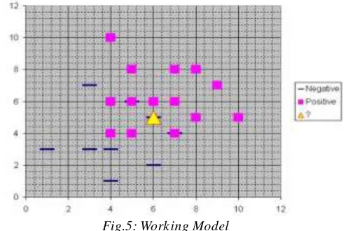
notion is that a foreseen target value of an article is probable to be about the similar as other articles that have close values of the predictor variables. Consider this figure 5.

Fig.5: Work ing Model

Now, suppose we are putting effort to forecast the value of a novel case signified by the triangle with predictor values x=6, y=5.1. Should we foresee the target as positive or negative? Observe that the triangle is position approximately precisely on top of a dash depicting a negative value. But that dash is in a quite strange position contrasted to the other dashes which are clu stered underneath the squares and left of center. So it could be that the fundamental negative value is an odd case.The adjacent neighbor classification operated for this instance depends on how many neighboring points are thought of. If 1-NN is exploited and only the closest point is considered, then obviously the novel point should be categorized as negative since it is on top of a known negative point. Conversely, if 9-NN classification is employed and the closest 9 points are considered, then the consequence of the surrounding 8 positive points may overbalance the close negative point.A Probabilistic Neural Network builds on this base and simplifies it to consider all of the other points. The distance is calculated from the point being analyzed to each of the other points, and a radial basis function (RBF) [11] (also called a

k ernel function) is put into the distance to compute the weight (influence) for each point.

3.1. Advantages and disadvantages of PNN networks:

1) It is typically much quicker to train a

PNN/GRNN network than a multilayer

perceptron network.

2) PNN/GRNN networks often are more precise

than multilayer perceptron networks.

3) PNN/GRNN networks are comparatively numb

to outliers (wild points).

4) PNN networks generate precise predicted target probability scores.

5) PNN networks come up to Bayes optimal

classification.

(5)

7) PNN/GRNN networks necessitate more memory

space to amass the model.

3.2.1. Removing unnecessary neurons

One of the drawbacks of PNN models contrasted to multilayer perceptron networks is that PNN models are huge because of the fact that there is one neuron for each training row. [14] This effects the model to run slower than multilayer perceptron networks when employing scoring to predict values for new rows . DTREG offers an alternative to cause it get rid of redundant neurons from the model after the model has been constructed.

Eliminating needless neurons has three reimbursements: 1. The size of the amassed sculpt is diminished. 2. The time necessary to apply the model during

scoring is lessened.

3. Detaching neurons often enhances the accuracy

of the model.

The process of eliminating pointless neurons is an iterative process. Leave-one-out validation is employed to measure the blunder of the model with each neuron being eliminated. The neuron that effects the least increase in error (or possibly the largest reduction in error) is then eliminated from the model. The process is recurred with the residual neurons until the stopping criterion is achieved.When superfluous neurons are rejected, the

“Model Size” section of the scrutiny report illustrates how

the error varies with various numbers of neurons. You can view a graphical chart of this by clicking Chart/Model size.There are three criteria that can be chosen to steer the exclusion of neurons:

1. Minimize error– If this option is preferred, then DTREG eliminates neurons as long as the leave-one-out error remains steady or decreases. It stops when it discovers a neuron whose exclusion would cause the error to increase above the minimum found.

2. Minimize neurons – If this option is preferred, DTREG excludes neurons until the leave-one-out error would surpass the error for the model with all neurons.

3. Number of neurons– If this option is preferred, DTREG diminishes the least significant neurons until only the specified number of neurons remain.

3.3 PNN:

NEWPNN generates a two layer network [6]. The first layer has RADBAS neurons, and computes its weighted inputs with DIST, and its net input with NETPROD. The second layer has COMPET neurons, and computes its weighted input with DOTPROD and its net inputs with NETSUM. Only the first layer has prejudices. NEWPNN sets the first layer weights to P', and the first layer biases are all set to 0.8326/SPREAD

effecting in radial basis functions that cross 0.5 at weighted inputs% of +/- SPREAD.

3.4 Methodol ogy:

An elucidation of the derivation of the PNN classifier was provided. PNNs had been utilized for categorization issues.[15] The PNN classifier offered good precision, very small training time, robustness to weight changes, and negligible retraining time. There are 6 stages involved in the projected prototype which are initiating from the data input to output. The initial stage is should be the image processing system. Principally in image processing system, image acquisition and image enhancement are the steps that have to do. In this manuscript, these two steps are skipped and all the images are composed from accessible resource. The proposed model necessitates transforming the image into a format capable of being influenced by the computer. The MR images are transformed into matrices form by using MATLAB. Then, the PNN is exploited to categorize the MR images. Finally, performance based on the outcome will be scrutinized at the end of the development stage.

IV. FUZZY CLUSTERING MODEL

Fuzzy clustering plays a vital position in resolving crisis in the domains of pattern identification and fuzzy model recognition [7]. A diversity of fuzzy clustering techniques have been projected and most of them are pertaining to the distance criteria. One predominantly employed algorithm is the Fuzzy C-Means (FCM) algorithm. It exploits reciprocal distance to evaluate fuzzy weights. A more competent algorithm is the new FCFM. It calculates the cluster center using Gaussian weights, utilizes large initial prototypes, and adds processes of eliminating, clustering and merging. In the subsequent sections we confer and contrast the FCM algorithm and FCFM algorithm.Spatial Fuzzy C Means method inte grates spatial data, and the membership weighting of each cluster is manipulated after the cluster distribution in the neighborhood is considered. The first pass is similar as that in standard FCM to compute the membership function in the spectral domain. In the second pass, the membership data of each pixel is mapped to the spatial domain and the spatial function is evaluated from that. The FCM iteration proceeds with the new membership that is integrated with the spatial function. The iteration is stopped when the maximum difference flanked by cluster centers or membership functions at two successive iterations is less than a least threshold value.

The Fuzzy C-Means (FCM) algorithm was initiated. The notion of FCM is employing the weights that diminishes the total weighted mean-square error by equation 6: J(wqk, z(k)) = (k=1,K) (k=1,K) (wqk)|| x(q)- z(k)||2

(6)

wqk = (1/(Dqk)2)1/(p-1) / (k=1,K) (1/(Dqk)2)1/(p-1) ,

p > 1 –eq(6)

The FCM permits each feature vector to fit in to every cluster with a fuzzy truth value (between 0 and 1), which is evaluated using Equation (6). The algorithm allocates a feature vector to a cluster in accordance to the maximum weight of the feature vector over all clusters [8].

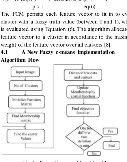
4.1 A New Fuzzy c-means Implementati on Algorithm Flow

Fig. 6: Fuzzy C-means Algorithm Flow.

In order to weigh against the FCM with FCFM, our execution permits the user to opt for initializing the weights using feature vectors or arbitrarily. The process of initializing the weights using feature vectors allocates the first Kinit (user-given) feature vectors to prototypes

then calculates the weights.

4.2 Standardize the Weights over Q.

During the FCM iteration, the evaluated cluster centers get closer and closer. To prevent the quick convergence and always clustering into one cluster as in equation 7.

w[q,k] = (w[q,k] – wmin)/( wmax– wmin) –eq(7)

before normalizing the weights over Q. Where wmax, wmin are maximum or minimum weights over the

weights of all feature vectors for the scrupulous class prototype.

4.3 Eliminating Empty Clusters.

In consequence to the fuzzy clustering loop we add a step to exclude the empty clusters. This step is put outside the fuzzy clustering loop and before computation of tailored XB validity. Without the abolition, the minimum distance of prototype pair utilized in Equation9 may be the distance of empty cluster pair. We entitle the method of abolishing small clusters by passing 0 to the process so it will only remove the empty clusters. In consequence to the fuzzy c-means iteration, for the rationale of contrast and to choose the optimal outcome, we add Step 9 to compute the group centers and the customized Xie-Beni clustering validity  :

The Xie-Beni validity is a product of compactness and separation measures [9],[10]. The compactness-to-separation ratio  is defined by Equation( 8) and (9).

 = {(1/K)(k=1,K)k2}/Dmin2 -eq(8)

k2 =(q=1,Q) wqk || x(q)–c(k) ||2 -eq(9)

Dmin is the minimum distance between the cluster centers.

The Modified Xie-Beni validity  is defined in equation (10).

= Dmin2/ {(k=1,K)k2 } –eq(10)

The variance of each cluster is computed by summing over only the members of each cluster rather than over all Q for each cluster, which compares with the unique Xie-Beni validity measure.

k2 ={q: q is in cluster k} wqk || x(q)–c(k) ||2 –eq(11)

The spatial function is comprised into membership function as given in Equation (11).

V. CONCLUSION

A new-fangled algorithm for Brain Tumor

Classification is proposed. This novel scheme is a blend of Dual tree Wavelet Transform, Probabilistic Neural Network and the fuzzy clustering with the implementation of GLCM. By employing these algorithms a competent Brain Tumor Classification technique was built with

maximum recognition rate. Simulation outcomes

exploiting Brain Tumor database illustrated the capability of the projected method for most favorable feature extortion and proficient Brain Tumor classification. The capability of our proposed Brain Tumor Classification system is established on the basis of acquired outcomes on Brain Tumor image database. On other Brain Tumor image databases the other grouping are there for training and test samples. In this proposal only 5 classes of Brain tumors are considered, with regard to an instance of 15 test images for example, but this technique can be extensive to more classes of Brain tumors.

REFERENCES

[1] N. Kwak, and C. H. Choi, “Input Feature Selection

for Classification Problems”, IEEE Transactions on

Neural Networks, 13(1), 143–159, 2002.

[2] Selesnick, Ivan W.; Baraniuk, Richard G.;

Kingsbury, Nick G. (November 2005). "The Dual-Tree Complex Wavelet Transform" (PDF). IEEE Signal Processing Magazine. 22 (6): 123–151. [3] B. Park, Y. R. Chen,” Co-occurrence Matrix

(7)

[4] D.F. Specht, “Probabilistic Neural Networks for Classification, mapping, or associative memory”, Proceedings of IEEE International Conference on Neural Networks, Vol.1, IEEE Press, New York, pp. 525-532, June 1988.

[5] D.F. Specht, “Probabilistic Neural Networks” Neural Networks, vol. 3, No.1, pp. 109-118, 1990. [6] Georgiadis. Et all , “ Improving brain tumor

characterization on MRI by probabilistic neural networks and non-linear transformation of textural

features”,Computer Methods and program in

biomedicine, vol 89, pp24-32, 2008

[7] Kaus M., “ Automated segmentation of MRI brain

tumors”, Journal of Radiology,vol. 218, pp. 585-591,2001

[8] Kornel, P., Bela, M., Rainer, S., Zalan, D., Zsolt, T.

and Janos, F.,“Application of neural network in medicine”, Diag. Med. Tech.,vol. 4,issue 3,pp: 538-540,1998.

[9] Mammadagha Mammadov ,Engin tas ,”An

improved version of backpropagation algorithm with effective dynamic learning rate and momentum

“ ,Inter.Conference on Applied Mathematics

,pp:356-361, 2006.

[10] Chien-Hsing Chou “A new cluster validity measure

and its application to image compression” July

2004, Pattern Analysis and Applications 7(2):205-220

[11] Orr M.J.L., Hallam J., Murray A., and Leonard .T,

“Assessing RBF networks using delve,"

International Journal of Neural Systems, vol. 10, issue 5, pp. 397-415, 2000.

[12] Sungheetha, Akey, and J. Suganthi. "An efficient clustering-classification method in an information gain NRGA-KNN algorithm for feature election of micro array data." Life Sci J 10.Suppl 7 (2013): 691-700.

[13] Sharma, Rajesh, and Akey Sungheetha.

"Segmentation and classification techniques of

medical images using innovated hybridized

techniques—a study." Intelligent Systems and Control (ISCO), 2017 11th International Conference on. IEEE, 2017.

[14] Sungheetha, Akey, and R. Rajesh Sharma. "Extreme Learning Machine and Fuzzy K-Nearest Neighbour Based Hybrid Gene Selection Technique for Cancer Classification." Journal of Medical Imaging and Health Informatics 6.7 (2016): 1652-1656.

[15] Beaula, A. Rajesh Sharma R., et al. "Comparative study of distinctive image classification techniques." Intelligent Systems and Control (ISCO), 2016 10th International Conference on. IEEE, 2016.

[16] J. Suganthi Akey Sungheetha, “Energy Saving

Optimized Polymorphic Hybrid Multicast Routing

Protocol.” International Review on Computers and

Softwares, Vol.8, No.6, pp. 1367 – 1373.

[17] Sungheetha, A., Mssujitha, R., Arthi, V., Sharma,

R.R. 2017, Data analysis of multiobjective

density based spatial clustering schemes in gene selection process for cancer diagnosis, Proceedings of 2017 4th International Conference on Electronics and Communication Systems, ICECS 2017.

[18] Sharma, Rajesh, P. S. Renisha, and Akey

Sungheetha. 2016 "Comparative Study on Medical Image Classification Techniques." International Journal of Advanced Engineering, Management and Science 2.11.

[19] Sharma, Rajesh, et al. 2016 "Effective Disaster Management by Efficient Usage of Resources." International Journal of Advanced Engineering, Management and Science 2.12.