www.hydrol-earth-syst-sci.net/15/3293/2011/ doi:10.5194/hess-15-3293-2011
© Author(s) 2011. CC Attribution 3.0 License.
Earth System
Sciences
On the return period and design in a multivariate framework
G. Salvadori1, C. De Michele2, and F. Durante3
1Dipartimento di Matematica, Universit`a del Salento, Provinciale Lecce-Arnesano, P.O. Box 193, 73100 Lecce, Italy 2DIIAR (Sezione CIMI), Politecnico di Milano, Piazza Leonardo da Vinci 32, 20132 Milano, Italy
3School of Economics and Management, Free University of Bozen-Bolzano, 39100 Bolzano, Italy
Received: 18 May 2011 – Published in Hydrol. Earth Syst. Sci. Discuss.: 10 June 2011 Revised: 5 October 2011 – Accepted: 24 October 2011 – Published: 4 November 2011
Abstract. Calculating return periods and design quantiles in a multivariate environment is a difficult problem: this pa-per tries to make the issue clear. First, we outline a possible way to introduce a consistent theoretical framework for the calculation of the return period in a multi-dimensional envi-ronment, based on Copulas and the Kendall’s measure. Sec-ondly, we introduce several approaches for the identification of suitable design events: these latter quantities are of utmost importance in practical applications, but their calculation is yet limited, due to the lack of an adequate theoretical envi-ronment where to embed the problem. Throughout the paper, a case study involving the behavior of a dam is used to illus-trate the new concepts outlined in this work.
1 Introduction
The notion of Return Period (hereinafter, RP) is frequently used in hydrology (as well as in water resources and civil engineering, and more generally in geophysical and environ-mental sciences) for the identification of dangerous events, and provides a means for rational decision making (for a re-view, see Singh et al., 2007, and references therein).
The traditional definition of the RP is as “the average time elapsing between two successive realizations of a prescribed event”, which clearly has a statistical base. Equally impor-tant is the related concept of design quantile, usually defined as “the value of the variable(s) characterizing the event asso-ciated with a given RP”. In engineering practice, the choice of the RP depends upon the importance of the structure, and the consequences of its failure. For example, the RP of a dam design quantile is usually 1000 years or more (Midttomme et al., 2001), while for a sewer it is about 5–10 years (Briere, 1999).
Correspondence to: G. Salvadori ([email protected])
While in the univariate case the design quantile is usu-ally identified without ambiguity – and widely used in the engineering practice (Chow et al., 1988) – in the multi-variate one this is not so. Indeed, the identification prob-lem of design events in a multivariate context is of funda-mental importance, but of troublesome nature. Recently, several efforts have been spent on the issues of multivari-ate design and quantiles (see, e.g. Serfling, 2002; Belzunce et al., 2007; Chebana and Ouarda, 2009, 2011b; Chaouch and Goga, 2010, and references therein; for a methodology to identify multivariate extremes by using depth functions see Chebana and Ouarda, 2011a). Here we address the following crucial question: “How is it possible to calculate the critical design event(s) in the multivariate case?” Below, we outline a suitable approach in order to provide consistent answers.
As we shall show later, the calculation of the RP is strictly related to the notion of Copula. The use of copulas in envi-ronmental sciences is recent and rapidly growing. Shortly, a multivariate copula Cis a joint distribution on Id= [0, 1]d with Uniform margins. The link between a multivariate dis-tribution F and the associated d-dimensional copula C is given by the functional identity stated by Sklar’s Theorem (Sklar, 1959):
F (x1, ..., xd) = C(F1(x1), ..., Fd(xd)) (1) for allx∈Rd, where theFi’s are the univariate margins ofF. If all theFi’s are continuous, thenCis unique. Most impor-tantly, theFi’s in Eq. (1) only play the role of (geometrically) re-mapping the probabilities induced byCon the subsets of
Id onto suitable subsets of Rd, without changing their val-ues: viz., the dependence structure modeled byC plays a central role in tuning the probabilities of joint occurrences. In fact, under weak regularity conditions, any pointx∈Rd
can be uniquely re-mapped ontou∈Id (and vice-versa) via the Probability Integral Transform:
For a thorough theoretical introduction to copulas see Joe (1997); Nelsen (2006); for a practical approach see Salvadori et al. (2007); Jaworski et al. (2010). In order to avoid trouble-some situations, hereinafter we shall assume thatF is contin-uous (but not necessarily absolutely contincontin-uous), and strictly increasing in each marginal: these regularity constraints are rather weak, and satisfied by the majority of the distributions used in applications. Clearly, also pathological cases can be carried out, but they require suitable techniques that go be-yond the scope of this work.
Later we shall use the Kendall’s distribution (or measure) functionKC:I→I (Genest and Rivest, 1993, 2001) given by
KC(t ) =P(W ≤ t ) = P(C(U1, ..., Ud) ≤ t ), (3) wheret∈Iis a probability level,W=C(U1, ..., Ud)is a uni-variate random variable (hereinafter, r.v.) taking value onI, and theUi’s are Uniform r.v.s onI with copulaC. Note that Eq. (3) practically measures the probability that a random event will appear in the region ofId defined by the inequal-ityC(u)≤t– see also Genest and Rivest (2001); Nappo and Spizzichino (2009). Thus, as we shall see,KC turns out to be a fundamental tool for calculating a copula-based RP for multivariate events.
Unfortunately, at present no general analytical expressions ofKC are known – except for special cases, like the one of bivariate Extreme Value copulas (Ghoudi et al., 1998), and some Archimedean copulas (McNeil and Neˇslehov´a, 2009) – and it is necessary to resort to simulations (see, e.g. Algo-rithm 1 outlined later).
The paper is organized as follows. In Sect. 2 we first il-lustrate the case study. In Sect. 3 we reconsider a previously introduced notion of RP in a multivariate environment, and compare it with other approaches. In Sect. 4 we show how to calculate the corresponding quantile. Then, in Sect. 5 we present two strategies to calculate critical design events in a multivariate context. Finally, in Sect. 6 we discuss the results outlined in the paper, and draw some conclusions.
2 The case study
Although this work is of methodological nature, we feel im-portant to illustrate with practical examples the new concepts introduced. For this reason, we first present the case study that will be used throughout the paper.
The data are collected at the Ceppo Morelli dam, and are essentially the same as those investigated in De Michele et al. (2005), to which we make reference for further de-tails. The dam, completed in 1929, is located in the valley of Anza catchment, a sub-basin of the Toce river (Northern Italy), and was built to produce hydroelectric en-ergy. The dam is characterized by a small water storage of about 0.47×10⁶m3. The minimum level of regulation is 774.75 m a.s.l., while the maximum is 780.75 m a.s.l. The
maximum water level is at 782.5 m a.s.l., and the dam crest level is at 784 m a.s.l. The dam has an uncontrolled spill-way (84 m long) at 780.75 m a.s.l., and also intermediate and bottom outlets (the latter ones are obstructed by river sediments).
In De Michele et al. (2005), “undisturbed” flood hydro-graphs incoming the reservoir were fixed by using the inverse reservoir routing, the water levels in the reservoir, and the operations on the controlled outlets. Then, maximum annual flood peaksQand volumesV were identified and selected for 49 years, from 1937 to 1994. As a result of a thorough investigation, almost all of the occurrence dates of theQ’s and the V’s were the same: i.e. they happened during the same flood event.
As an improvement over De Michele et al. (2005), beyond the pair (Q,V), also the initial water levelLin the reservoir before the flood event (Q,V) is considered in this work, in order to analyse the triplet (Q,V,L) of practical interest: in fact, on the one handL represents the starting state of the dam; on the other hand, (Q,V) is the hydrologic “forcing” to the structure. Clearly, there are physical reasons to assume thatLis independent of (Q,V) – see also below. The sample mean ofLis about 780.44 m a.s.l., with a sample standard de-viation of about 1 m. The small variability ofLwith respect to its range (here [774.75, 780.75] is the regulation range), is mainly due to the management policy of the reservoir: the target of the dam manager is to keep a high water level, in order to get the maximum benefit concerning the production of electric energy.
Using the pair (Q,V), it is possible to calculate the associ-ated flood hydrograph with peakQand volumeV, once the shape of the hydrograph has been chosen. As first approx-imation, it is possible to consider a triangular shape, where the base time is equal toTb= 2V /Q, the time of rise equals Tr=Tb/2.67, and the time of recession is equal to 1.67Tr,
(see Soil Conservation Service, 1972 and Chow et al., 1988, p.229 – for a different approach see Serinaldi and Grimaldi, 2011). Consequently, the flood hydrographqis given by
q(t ) =
(
1.335t Q2V , 0 ≤ t ≤ Tr
1.6Q−0.8t Q2V , Tr ≤ t ≤ Tb .
Later, in Sect. 5, we shall test the behavior of the dam sub-ject to selected hydrographs. More particularly, we shall first operate the reservoir routing of the flood hydrograph (see, e.g. Bras, 1990, p.475–478 and Zoppou, 1999) considering as outlet only the uncontrolled spillway, and then we shall check whether or not the reservoir level exceeds the crest level of the dam.
0 100 200 300 400 500 0
20
40 777
778 779 780 781 782
Q Observed events
V
L
0 100 200 300 400 500
0 0.2 0.4 0.6 0.8 1
Q (m3/s)
F Q
Peak Flow
Empirical GEV Low. 95% C.B. Upp. 95% C.B.
0 10 20 30
0 0.2 0.4 0.6 0.8 1
V (106 m3)
FV
Peak Volume
Empirical GEV Low. 95% C.B. Upp. 95% C.B.
775 780 785
0 0.2 0.4 0.6 0.8 1
L (m.a.s.l.)
FL
Initial Level
[image:3.595.124.465.65.339.2]Empirical Kernel Fit Overtopping
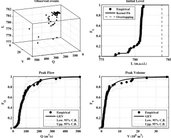
Fig. 1. Trivariate plot of the available (Q,V,L) observations, and fits of the marginal distributions – see text.
the estimates of the parameters are reported in Table 1. The fits are valuable, as they passed standard goodness-of-fit tests (namely, Kolmogorov-Smirnov and Anderson-Darling – see, e.g. Kottegoda and Rosso, 1997) at all usual levels (viz., 1 %, 5 %, and 10 %). Instead, the behavior of the variableL is quite tricky (as explained above, the water level is arbitrarily fixed by the dam manager): for this reason, its law is calcu-lated via a non-parametric Normal Kernel estimation (Bow-man and Azzalini, 1997). As a result, also in this case the Kolmogorov-Smirnov test is passed at all usual levels.
The trivariate plot of the observations, as shown in Fig. 1, is the first step usually carried out by practitioners to inves-tigate the multivariate behavior of the phenomenon. How-ever, we want to stress that this type of graph only provides partial information, and should not be used to draw rough conclusions about the dependence structure of (Q,V,L) – see below, and also Genest and Favre (2007) for a thorough review.
In order to investigate the joint behavior of the variables (Q,V,L), as is typical in copula analysis, we shall use the normalized ranks to carry out a non-parametric study. The trivariate rank-plot shown in Fig. 2 provides some rough in-dications about the global dependence structure (i.e. the cop-ula) linking the three variables (Q,V,L).
As already mentioned above, there are physical reasons to assume thatL is independent of (Q,V): the rank-plots shown in Fig. 2 support this fact. Indeed, the sample is rather uniformly sparse in both the (Q,L) and (V,L) planes. Also,
Table 1. Maximum-Likelihood estimates of the GEV parameters
forQandV, and corresponding 95% Confidence Intervals.
Variable Shape Scale Position
Q 0.3677 36.2031 59.3507 (m3s−1) – (m3s−1) (m3s−1) 95% C. I. [0.15, 0.58] [27.57, 47.55] [48.15, 70.55]
V 0.6149 1.5246 1.7231
(106m3) – (106m3) (106m3) 95% C. I. [0.37, 0.86] [1.10, 2.11] [1.26, 2.19]
the estimates of the Kendall’s τ and the Spearman’sρ are not statistically significant (as confirmed by the correspond-ingp-values), and formal tests of independence suggest to accept the hypothesis thatL is independent of (Q,V). On the contrary, the variables (Q,V) are significantly positively associated, and thusQandV are not independent: the esti-mates of both the Kendall’sτ and the Spearman’sρare large, and the correspondingp-values are negligible (see the values reported in Fig. 2).
As in De Michele et al. (2005), a Gumbel copula was used to model the dependence betweenQandV, with parame-terθ≈3.1378, calculated via the inversion of the Kendall’s
[image:3.595.312.542.417.515.2]0 0.25 0.5 0.75 1 0
0.25 0.5
0.75 1 0
0.25 0.5 0.75 1
Q Ranks (Q,V,L)
V
L
0 0.25 0.5 0.75 1
0 0.25 0.5 0.75 1
Q
V
Ranks (Q,V)
τe≈0 . 6 5 5
p- v .≈3 . 9 5 e- 1 1
ρe≈0 . 7 9 9
p- v .≈5 . 9 e- 1 2
0 0.25 0.5 0.75 1
0 0.25 0.5 0.75 1
L
Q
Ranks (L,Q)
τe≈- 0 . 0 7 7 3
p- v .≈0 . 4 4
ρe≈- 0 . 1 1 1
p- v .≈0 . 4 5
0 0.25 0.5 0.75 1
0 0.25 0.5 0.75 1
L
V
Ranks (L,V)
τe≈0 . 0 9 5 8
p- v .≈0 . 3 4
ρe≈0 . 1 2 8
[image:4.595.129.469.62.338.2]p- v .≈0 . 3 8
Fig. 2. Trivariate rank-plot of the available (Q,V,L) observations, and bivariate rank-plots of the marginals – see text. Also shown are the estimates of the Kendall’sτand the Spearman’sρ, as well as the correspondingp-values (derived from non-parametric tests of independence based on rank statistics).
2009; Genest et al., 2009; Kojadinovic et al., 2011): the re-sulting largep-values indicate that the Gumbel copulaCQV cannot be rejected at all standard levels. As a matter of facts, the analysis of the (Q,V) rank-plot in Fig. 2 shows a signif-icant association between these two variables in the upper-right corner of the unit square: indeed, the extreme pairs practically lie on the main diagonal. Thus, it is not a sur-prise that the fitted Gumbel copula, having a large upper tail dependence coefficientλUpp≈0.75 (Nelsen, 2006; Salvadori
et al., 2007) is suitable for modeling the dependence structure of the pair (Q,V). In passing, note thatCQV is an Extreme Value copula (Nelsen, 2006): since bothFQandFV are GEV distributions, it turns out thatFQV=CQV(FQ, FV)is a bi-variate Extreme Value law (after all, Q andV are annual maxima).
Given the previous results, sinceLcan be assumed to be independent of (Q,V), it is immediate to construct a suitable trivariate copulaCQV Lto model the dependence structure of the triplet (Q,V,L):
CQV L(u, v, w) = CQV(u, v) w, (4)
where (u, v, w)∈I3. As above, the ability of this cop-ula to model the trivariate data is properly checked, and the resulting large p-values indicate that it cannot be re-jected at all standard levels. In passing, note that also
CQV L is an Extreme Value copula. In addition, sinceCQV
is Archimedean (Nelsen, 2006), then CQV L is a partic-ular case of a “nested” Archimedean copula (Joe, 1997; Grimaldi and Serinaldi, 2006; Serinaldi and Grimaldi, 2007; H¨ardle and Okhrin, 2010; Hering et al., 2010). However,
FQV L=CQV L(FQ, FV, FL) is not a trivariate Extreme Value law, sinceFLis not a GEV distribution.
3 Return period in a multivariate framework
In order to provide a consistent theory of RP’s in a multi-variate environment, it is first necessary to precisely define the abstract framework where to embed the question. Pre-liminary studies can be found in Salvadori (2004); Salvadori and De Michele (2004); Durante and Salvadori (2010); Sal-vadori and De Michele (2010), and some applications are presented in De Michele et al. (2007); Salvadori and De Michele (2010); Vandenberghe et al. (2010). Hereinafter, we shall consider as the object of our investigation a sequence
X={X1,X2, ...}of independent and identically distributed d-dimensional random vectors, withd >1: thus, eachXihas the same multivariate distributionF as of the random vector
Volume, joined by the copulaC. The case of a non-stationary sequenceX is rather tricky, and will be discussed in a future work.
In applications, usually, the event of interest is of the type
{X∈D}, whereDis a non-empty Borel set inRdcollecting all the values judged to be “dangerous” according to some suitable criterion. Note that the Borel family includes all the sets of interest in practice (like, e.g. the intervals(−∞, x1), (x1, x2),(x2, ∞), as well as the corresponding
multivari-ate versions). Letµ >0 be the average inter-arrival time of the realizations inX (viz.,µis the average time elapsing be-tweenXiandXi+1). Following, e.g. Embrechts et al. (2003),
and given the fact that the sequenceXis i.i.d. (and, thus, sta-tionary), the univariate r.v.’s{Bi=ID(Xi)}form a Bernoulli process (whereI is an indicator set function), with positive probability of “success”pDgiven by
pD = P(X ∈ D), (5)
where we assume that 0< pD<1. Then, it makes sense
to calculate the first random time AD that the sequence B={B1, B2, ...}, generated byX, takes on the value 1 (viz.,
the first random time thatXentersD):
AD = µ· min{i : Xi ∈ D}. (6)
Clearly, the r.v.AD/µfollows a Geometric distribution with
parameterpD, and therefore the expected value ofADis
E(AD)= µD = µ/pD. (7)
Given the well known “memoryless property” of the Geo-metric distribution, and the features of the Bernoulli process (see, e.g. Feller, 1971), it is clear thatµDalso corresponds to the average inter-arrival time between two successive re-alizations of the event{X ∈ D}. Evidently,µD ranges in [µ, + ∞): for example, if annual maxima are investigated, then µ= 1 year, and hence µD= 1/pD≥µ. We are now
ready to introduce a consistent notion of RP.
DEFINITION 1. The RP associated with the event{X∈D}
is given byµD=µ/P(X∈D).
Definition 1 is a very general one: the setDmay be con-structed in order to satisfy broad requirements, useful in dif-ferent applications. Indeed, most of the approaches already present in literature are particular cases of the one outlined above.
As a univariate example, letXbe a r.v. with distribution
FX. In order to identify a dangerous region, traditionally a prescribed critical design valuex∗is used. Then,D(or,
bet-ter,Dx∗) contains all the realizations that are judged to be
“more dangerous” than x∗. For instance, in hydrology, if droughts are of concern,x∗may represent a small value of river flow, and the dangerous realizations of interest are those for which X≤x∗ (viz., Dx∗= [0, x∗]). Instead, if floods
are of concern,x∗may indicate a large value of river flow, and the dangerous realizations of interest are those for which
X≥x∗(viz.,Dx∗=[x∗,∞)). According to Definition 1, the
corresponding RP’s are µ/FX(x∗)in the former case, and
µ/(1−FX(x∗))in the latter one.
It is important to stress that the RP is a quantity associ-ated with a proper event. However, with a slight abuse of language, we may also speak of “the RP of a realization” (viz.,x∗ in the example given above), meaning in fact “the RP of the event{Xbelongs to the dangerous regionDx∗
iden-tified by the given realizationx∗}”. Indeed, in a univariate framework, the assignment ofx∗uniquely specifies the cor-responding regionDx∗.
Actually, also in a multivariate framework it is possible to associate a given multi-dimensional realization x∗∈Rd
with a dangerous region Dx∗⊂Rd. As an illustration,
consider the two different bivariate dangerous regions con-structed in Salvadori (2004); Salvadori and De Michele (2004). In these papers the joint behavior of the vector
(X, Y )∼F=C(FX, FY) was analysed: for instance, in terms of variables of hydrological interest, think of the pairs flood peak-volume, or storm intensity-duration. In particular, great attention was paid to the following two sets:
1. (“OR” case)D∨
z∗={(x, y)∈ R2: x > x∗∨y > y∗},
where at least one of the components exceeds a pre-scribed threshold (roughly, it is enough that one of the variables is too large);
2. (“AND” case)D∧
z∗={(x, y)∈R2: x > x∗∧y > y∗},
where both the components exceed a prescribed thresh-old (roughly, it is necessary that both variables are too large).
Herez∗= (x∗,y∗) is a prescribed vector of thresholds, and
∨,∧are the “(inclusive) OR” and “AND” operators. In this work we follow a different approach. The idea stems from the possibility to write, in the univariate case, the dangerous region Dx∗ in two equivalent ways: either
asDx∗={x:x≥x∗}, orDx∗={x:FX(x)≥FX(x∗)}. Clearly,
the same rationale holds by considering as a dangerous re-gion the set Dx∗={x:x≤x∗}, which may be of interest,
e.g. for the study of droughts. Then, by considering the above formulation as given in terms of the distribution functionFX, it is clear how it can be extended in a natural way to the multi-dimensional case, as we shall illustrate below. First of all we need to introduce the following notion.
DEFINITION 2. Given a d-dimensional distribution
F=C(F1, ..., Fd)and t∈(0, 1), the critical layer LFt of leveltis defined as
LF
t = {x ∈ Rd : F (x) = t}. (8) Clearly, LF
t is the iso-hyper-surface (having dimension
d−1) where F equals the constant valuet: thus, LF t is a (iso)line for bivariate distributions, a (iso)surface for trivari-ate ones, and so on. Evidently, for any givenx∈Rd, there exists a unique critical layerLF
one identified by the level t=F (x). Note that, thanks to Eq. (2), there exists a one-to-one correspondence between the two iso-hyper-surfacesLC
t ={u ∈ Id : C(u)=t} (per-taining toCinId) andLF
t (pertaining toF inRd). The critical layer LF
t partitions Rd into three non-overlapping and exhaustive regions:
1. R<
t ={x ∈ Rd : F (x) < t}; 2. LF
t , the critical layer itself; 3. R>
t ={x ∈ Rd : F (x) > t}.
Practically, at any occurrence of the phenomenon, only three mutually exclusive things may happen: either a realization of
Xlies inR<
t , or overLFt , or it lies inR>t . Note that all these three regions are Borel sets.
Thanks to the above discussion, it is now clear that the following (multivariate) notion of RP is meaningful, and co-incide with the one used in the univariate framework.
DEFINITION 3. LetXbe a multivariate r.v. with distri-butionF=C(F1, ..., Fd). Also, letLFt be the critical layer supporting a realizationxofX(i.e.t=F (x)). Then, the RP associated withxis defined as
1. for the regionR> t
Tx> = µ/P X ∈ R>t
, (9)
2. for the regionR< t
Tx< = µ/P X ∈ R<t
. (10)
In the sequel we shall concentrate only uponR>
t : the cor-responding formulas forR<
t could easily be derived. Note thatR>
t may be of interest, e.g. when floods are investigated, whileR<
t may be appropriate if droughts are of concern. Now, in view of the results outlined in Nelsen et al. (2001, 2003), it is immediate to show that
Tx>= µ
νF({x ∈ Rd : F (x) > t})
= µ
1−νF({x ∈ Rd : F (x)≤ t})
= µ
1−KC(t )
,
(11)
whereνF is the probability measure induced byF overRd, andKCis the Kendall’s distribution function associated with
C (see Eq. 3 and the ensuing discussion). Clearly, Tx> is a function of the critical level t identified by the relation
t=F (x). It is then convenient to denote the above RP via a special notation as follows.
DEFINITION 4. The quantity κx=Tx> is called the Kendall’s RP of the realization x belonging to LF
t (here-inafter, KRP).
F ≡ t F ≡ s
x* y*
z*
D∧
z∗
[image:6.595.316.534.64.258.2]w* "AND" case
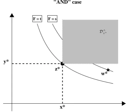
Fig. 3. Graphical illustration of the dangerous regionD∧
z∗(shaded)
in the “AND” case – see text.
An advantage of the approach outlined in this work is that realizations lying over the same critical layer do always gen-erate the same dangerous region. Evidently, this is not the case considering the “OR–AND” approach discussed above. Furthermore, in the “AND” case, it may happen that real-izations not lying in the dangerous regionDz∗of interest have
a RP larger than the one ofz∗. More specifically, as graphi-cally illustrated in Fig. 3, for a given realizationz∗lying on the isoline of levelt∈(0, 1) (where F≡t), the dangerous regionD∧
z∗is given by the shaded area. However, given
an-other realizationw∗, lying on the isoline of levels > t, the corresponding RP may be larger than the one ofz∗, butw∗
does not belong toD∧
z∗. A similar rationale also holds for the
“OR” case. Instead, in the approach outlined in this work, all the realizationsyhaving a KRPκy< κx must lie inR<t , whereas all thosey having a KRPκy> κx must lie inR>t – clearly, all the realizations lying overLF
t share the same KRPκx.
For the sake of convenience, we report below the algo-rithm explained in Salvadori and De Michele (2010) for the calculation ofKC(see also Genest and Rivest, 1993; Barbe et al., 1996), which yields a consistent Maximum-Likelihood estimator ofKC. Here we assume that the copula model is well specified, i.e. it is available in a parametric form.
ALGORITHM 1. Calculation of the Kendall’s measure functionKC.
1. Simulate a sample u1, ..., um from the
d-copula C.
2. For i=1, ..., m calculate vi=C(ui). 3. For t∈I calculate
b
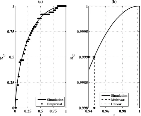
As an illustration, in Fig. 4a we plot an estimate of the functionKC associated with the copulaCQV L: here Algo-rithm 1 is used, running a simulation of size m= 5×10⁷. Also shown is the empirical estimate ofKC calculated by using the available observations: the horizontal patterns are simply due to the small sample size.
4 Quantiles associated with the KRP
Traditionally, in the univariate framework, once a RP (say,
T) is fixed (e.g. by design or regulation constraints), the corresponding critical probability level p is calculated as 1−p=P(X > xp)=µ/T, and by invertingFXit is then im-mediate to obtain the quantilexp=FX(−1)(p), which is usu-ally unique. Then,xpis used in practice for design purposes and rational decision making. As shown below, the same ap-proach can also be adopted in a multivariate environment (to be compared with Belzunce et al., 2007).
DEFINITION 5. Given ad-dimensional distributionF=
C(F1, ..., Fd)withd-copulaC, and a probability levelp∈I, the Kendall’s quantileqp∈I of orderpis defined as
qp = inf{t ∈ I : KC(t ) = p} = KC(−1)(p), (12) whereKC(−1)is the inverse ofKC.
Definition 5 provides a close analogy with the definition of univariate quantile: indeed, recall thatKC is a univariate distribution function (see Eq. 3), and henceqpis simply the quantile of orderpofKC. Thanks to Eq. (2), it is clear that the critical layerLF
qpis the iso-hyper-surface inRdwhereF takes on the valueqp, whileLCqp is the corresponding one in
Idwhere the related copulaCequalsqp. Now, let LF
qp be fixed. Then, according to Eq. (3),
p=KC(qp)=P(C(F1(X1), ..., Fd(Xd)) ≤ qp). Therefore,
pis the probability measure induced byCon the regionR< qp, while (1−p) is the one ofR>
qp. From a practical point of view this means that, in a large simulation ofnindependent
d-dimensional vectors extracted fromF, np realizations are expected to lie inR<
qp, and the others inR > qp.
REMARK 1. It is worth stressing that a common error is to confuse the value of the copulaC with the probabil-ity induced byC onId (and, hence, on Rd): on the criti-cal layerLCqp it isC=qp, but the corresponding regionR<
qp has probabilityp=KC(qp)6=qp, sinceKC is usually non-linear (the same rationale holds for the regionR>
qp). In other words, while in the univariate case the valuep=FX(xp) cor-responds to the probability induced on the regionR<
p, where
xpis the quantile ofXof orderp, this is not so in the multi-variate case.
SinceKCis a probability distribution, andqpis the corre-sponding quantile of orderp, we could use a standard boot-strap technique (see, e.g. Davison and Hinkley, 1997) to es-timate qp if it cannot be calculated analytically. The idea is simple, and stems directly from the very definition ofqp:
0 0.25 0.5 0.75 1
0 0.25 0.5 0.75 1
t
KC
(a)
Simulation Empirical
0.94 0.96 0.98 1
0.998 0.9985 0.999 0.9995 1
t
KC
(b)
Simulation Multivar. Univar.
Fig. 4. (a) Simulation-based estimate of the function KC (con-tinuous line) associated with the copula CQV L; also shown is its empirical estimate (markers) calculated by using the available observations – see text. (b) Plot of the (millenary KRP) quantile
t∗≈0.946537 (thick-dashed line) associated with the critical prob-ability levelp= 0.999; also shown (thin-dashed line) is the esti-mate of the valueKC≈0.999998 associated with the critical level
t1D∗ ≈0.997754 – see text.
viz., to look for the valueqpofCsuch that, in a simulation of sizen, np realizations show a copula value less thanqp. Then, by performing a large number of independent simula-tions of sizen, the sample average of the estimatedqp’s is expected to converge to the true value ofqp. A possible al-gorithm is given below, most suitable for vectorial software. Here we assume that the copula model is well specified, i.e. it is available in a parametric form.
ALGORITHM 2. Calculation ofqp. First of all, choose a sample sizen, a critical probability levelp, the total number of simulationsN, and fix the critical indexk=bnpc.
for i= 1:N
S= sim (C; n); % simulate n d-vectors from copula C
C=C(S); % calculate C for simulated vectors
C= sort (C); % sort-ascending simulated C values
E(i)=C(k); % store new estimate of qp into vector E
end
q= Mean(E); % calculate the estimate of
qp
[image:7.595.310.546.64.259.2]yield an approximate confidence interval forqp (see DiCi-ccio and Efron, 1996 for more refined solutions): for in-stance, at a 10 % level, the random interval (q0.05, q0.95)
can be used, where q0.05 and q0.95 are, respectively, the
quantiles of order 5 % and 95 % extracted from the vector
E. Using Algorithm 2 (and settingn= 104,p= 0.999, and
N= 107, for a total of 1011simulated triplets), we estimated
q0.999≈0.946537 for the copulaCQV Lof interest here, and a 10 % confidence interval (0.946110, 0.946973), a process that took about 48 h of CPU time on a iMac equipped with a 3.06 GHz Intel Core 2 Duo processor and 8 GB RAM. As an illustration, in Fig. 4b we show an estimate of the func-tionKC, associated with the copulaCQV L, att∗≈0.946537 (corresponding to a millenary KRP): as expected, the value
KC(t∗)is almost exactly equal to 99.9 %.
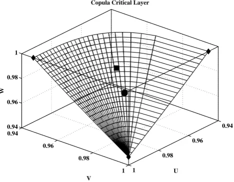
As a further illustration, in Fig. 5 we plot the critical iso-surfaceLC
t∗of the trivariate copulaCQV Lfor the critical level
t∗≈0.946537, corresponding to a regulation return period of 1000 years (viz., all the realizations onLC
t∗ have a KRP
equal to 1000 years). Then, CQV L=t∗ for all points be-longing toLCt∗. Instead, CQV L< t∗ (andκx<1000 years)
in the regionR<
t∗ “below” LCt∗, the one containing the
ori-gin 0 = (0, 0, 0), whereasCQV L> t∗(andκx>1000 years) in the regionR>
t∗ “above”LCt∗, the one containing the
up-per corner 1 = (1, 1, 1). On average, only 0.1 % of the real-izations extracted from a simulation ofCQV L are expected to lie in R>
t∗. However, the level of the critical layer is t∗=q0.999≈0.946537<p = 0.999, as indicated by the
dia-monds markers in the plot.
As a further example, consider that the regionR>
0.999
iden-tified by the critical layerLF
0.999(where the multivariate
dis-tribution F, or, equivalently, the copula C, takes on the value 0.999) has an estimated probability smaller than 10−6, and a corresponding KRP of about 3×10⁶years: practically, only one realization ofCQV L out of 3×10⁶simulations is expected to lie in R>
0.999 (instead of 1 out of 1000).
Evi-dently, ifF(orC) were substituted forKCin Eq. (11) during the design phase, then the structure to be constructed would result over-sized (being expected to withstand stunning ex-treme events).
5 Design in a multivariate framework
The situation outlined in the previous section is generally similar to the one found in the study of univariate phenom-ena, where a single r.v. X with distributionFX is used to model the stochastic dynamics. However, as already men-tioned, the multivariate case generally fails to provide a nat-ural solution to the problem of identifying a unique design realization. In fact, even if also the layerLF
t acts as a (multi-dimensional) critical threshold, there is no natural criterion to select which realization lying onLF
t (among the∞d
−1
pos-sibilities) should be used for design purposes. In other words, in a multivariate environment, the sole tool provided by the
0.94 0.96 0.98 1
0.94
0.96
0.98
1 0.94
0.96 0.98 1
U Copula Critical Layer
V
[image:8.595.311.546.64.246.2]W
Fig. 5. Critical iso-surfaceLCt∗of the copulaCQV Lcorresponding to the (millenary KRP) critical levelt∗≈0.946537, indicated by the diamond markers on the axes. The circle and the square mark-ers indicate, respectively, the Component-Wise and the Most-Likely design realizations – see text.
RP may not be sufficient to identify a design realization, and additional considerations may be required in order to pick out a “characteristic” realization over the critical layer of in-terest. In the following, we outline possible ways to carry out such a selection. Clearly, several approaches can be pro-posed, each one possibly yielding a different solution: below, we show two possible elementary strategies to deal with the problem.
The basic idea is simply to introduce a suitable function (say,w) that “weighs” the realizations lying on the critical layer of interest. Following this approach, the practitioner can then freely choose the criterion (i.e. the functionw) that best fits the practical needs. Clearly, without loss of general-ity,wcan be assumed to be non-negative. In turn, a “design realization” can be defined as follows.
DEFINITION 6. Letw: LF
t →[0,∞) be a weight func-tion. The design realizationδw ∈ LFt is defined as
δw(t ) = argmax
x∈LF
t
w(x), (13)
provided that the argmax exists and is finite. Definition 6 deserves some comments.
Ghoudi et al., 1998). However, in general, the critical layers of such copulas will have a different geometry, and, in turn, will provide different design realizations. – The search of the point of maximum in Eq. (13) can be
subjected to additional constraints, in order to take into account the possible sensitivity of the structure under design to the behavior of specific marginals (see also the discussion in Remark 2): for instance, a Bayesian approach might be advisable.
– Sometimes it could be more appropriate to select a set of possible design realizations (i.e. an ensemble, rather than a single one) that should be used, together with experts’ opinions, in order to better evaluate the features of the phenomenon affecting the structure under design. This procedure can be carried out by using a suitable step function in Eq. (13).
In passing, we note that, in the present case study, the distributionFQV L and the copulaCQV L are trivariate, and hence the corresponding critical layers are simply two-dimensional surfaces inR3 andI3, respectively. Figure 5 shows the critical layer of levelt∗pertaining toCQV L, and the corresponding one pertaining toFQV L can be drawn by exploiting Eq. (2). Now, for the sake of graphical illustra-tion, it is possible to parametrize LF
t∗ in polar coordinates
(say,(α, r)) via a one-to-one transformation, and thus re-map and plot any functionwdefined overLF
t∗ onto the rectangle (0, π/4)×(0,r˜), for a suitable maximum rayr˜. In turn, it is rather easy to have a peek of the behavior of any weight functionwoverLF
t∗.
REMARK 2. A delicate problem may arise when adopt-ing the approach outlined above: to make the point clear, consider the following example. Suppose that we use the du-ration of a storm and the storm intensity as the two variables of interest. In a fast responding system (e.g. a sewer struc-ture), a storm having short duration but high intensity may cause a failure, whereas the same storm may not cause any problem at a catchment level. In the catchment, however, a storm with long duration and intermediate to low intensity may cause a flood event, whereas the same storm does not cause any problem to the sewer system. Now, as a matter of principle, the design realizationδw for the given return period (i.e. the “typical” critical storm calculated according to the strategy illustrated here) may not cause any problem in both systems, and therefore these would be wrongly de-signed. Practically, the sewer systems should be designed using critical design storms of short durations and high in-tensities, whereas a structure in the main river of the water-shed should be designed using storms of long durations and low intensities. However, the problem is more apparent than real. In fact, there are neither theoretical nor practical limita-tions to restrict the search for the maxima in Eq. (13) over a suitable sub-region ofLF
t∗: remember that all the realizations
on the critical layer share the same prescribed KRP. Thus,
when a sewer system is of concern, only storms having short durations and high intensities could be considered, whereas a critical design storm for a structure in the main river could be spotted by restricting the attention to storms of long dura-tions and low intensities. Roughly speaking, in the approach outlined here, the calculation of the critical design realization can be made dependent on both the environment in which a structure should be designed, as well as on the stochastic dy-namics of the phenomenon under investigation.
Overall, the procedure to identify the design realization could be described as follows. LetX be a random vector with distributionF=C(F1, ..., Fd).
1. Fix a RPT.
2. Calculate the corresponding probability level
p= 1−µ/T.
3. Compute the Kendall’s quantileqpas in Eq. (12), either analytically or by using Algorithm 2.
4. Fix a suitable weight functionw.
5. Calculate the point of maximumδwofwon the critical layerLF
qp.
The resultingδwrepresents a “typical” realization inRdwith a given RP. Roughly speaking, it denotes the design realiza-tion obtained by considering the very stochastic dynamics of the phenomenon. Note that, in general,δw(or, better, the cor-responding critical layer) should be considered together with other information (e.g. the physical features of the structure) in order to be correctly used in practice. For the sake of il-lustration, below we introduce two weight functions. 5.1 Component-wise excess design realization
A realization lying on the critical layerLF
t may be of ma-jor interest when all of its marginal components are ex-ceeded with the largest probability. In simple words, we sug-gest to look for the point(s)x=(x1, ..., xd)∈LFt such that it is maximum the probability that a dangerous realization
y=(y1, ...,yd) satisfies all the following component-wise inequalities:
y1 ≥ x1, ..., yd ≥ xd, (14)
ory>x using a simplified notation. The next definition is immediate.
DEFINITION 7. The Component-Wise Excess weight functionwCEis defined as
wCE(x) =P(X ∈ [x,∞)), (15)
Table 2. Estimates of the critical design realizations, for a
mil-lenary return period, according to different strategies – see text. Also shown are the estimates of the univariate quantiles of order
p= 0.999 of the variables of interest. The right-most column shows the Maximum Water Level of the dam associated with the flood event (Q,V,L) reported on the corresponding row.
Strategy Q V L M. W. L.
(m3s−1) (106m3) (m a.s.l.) (m a.s.l.) C.-E. 352.76 25.21 781.25 782.08 M.-L. 316.23 19.64 781.29 781.98
F·(−1)(0.999) 1208.9 172.58 781.44 784.80
Then, by restricting our attention to the critical layerLF t , the following definition is immediate.
DEFINITION 8. The Component-wise Excess design real-izationδCEof leveltis defined as
δCE(t ) = argmax
x∈LF
t
wCE(x), (16)
wheret∈(0, 1).
REMARK 3. Via the Probability Integral Transform and Sklar’s Theorem, it is easy to show that
wCE(x)= P(U ∈ [u(x),1]), (17)
where U has the same copula C as of X and Uniform marginals, u(x)=(F1(x1), ..., Fd(xd)), and [u, 1] is the hyper-rectangle inIdwith lower corneruand upper corner 1. Thus, the probabilities of interest can be directly computed in the unit hyper-cube (see, e.g. Joe, 1997) by working directly on the critical layerLC
t (instead ofLFt ), a solution numer-ically more convenient. Note that, for larged-dimensional problems, the CPU time involved may become prohibitive, though clever solutions have been proposed for larged’s (see, e.g. Cherubini and Romagnoli, 2009). In some cases,δCE
can be calculated analytically; otherwise, it can be empiri-cally estimated (e.g. by calculating it over suitable points of
LCt orLF t ).
In Fig. 6 we show the behavior ofwCEoverLFt∗, as well as
the Component-wise Excess design realizationδCE(t∗)
cal-culated for the case study investigated here (see also Fig. 5). This point has the largest probability to be component-wise exceeded by an extreme realization with KRP larger than 1000 years, and therefore it should be regarded as a sort of (statistical) “safety lower-bound”: viz., the structure under design should, at least, withstand realizations having (multi-variate) sizeδCE(t∗), as reported in Table 2.
As anticipated in Sect. 2, using the design realization
δCE(t∗), we operated the reservoir routing of the
corre-sponding flood hydrograph. Then, we checked whether or not the reservoir level exceeds the crest level of the dam
0 0.5 1
1.5 0
0.02
0.04
0.06 0
1 2 3 4
x 10−4
α
Excess probability over Critical layer
r
[image:10.595.48.285.140.212.2]PCE
Fig. 6. Polar re-mapped plot of the Component-Wise Excess weight
functionwCEover the critical layerLFt∗, corresponding to the
(mil-lenary KRP) critical levelt∗≈0.946537. The star marker indicates where the maximum is attained – see text and Table 2.
(i.e. 784 m a.s.l.). The column“M. W. L.” in Table 2 re-ports the value 782.08 m a.s.l.: thus, no over-topping occurs, i.e. the dam seems to be safe against Component-Wise Ex-cess millenary realizations.
5.2 Most-likely design realization
A further approach to the definition of a characteristic design event consists in taking into account the density of the mul-tivariate distribution describing the overall statistics of the phenomenon investigated: in fact, assuming that the density
f ofF is well defined overLF
t , we may think of using it as a weight function.
Clearly, the restrictionft of f over LFt is not a proper density, since it does not integrate to one. However, it may provide useful information, since it induces a (weak) form of likelihood overLF
t : in fact, it can be used to weigh the realizations lying onLF
t , and spot those that are (relatively) “more likely” than others. Indeed,ft inherits all the features of interest directly from the true global densityf. The next definition is immediate.
DEFINITION 9. The Most-Likely weight functionwMLis
defined as
wML(x) = f (x), (18)
wheref is the density ofF=C(F1, ..., Fd).
DEFINITION 10. The Most-Likely design realizationδML
of leveltis defined as
δML(t ) = argmax
x∈LF
t
wML(x) = argmax
x∈LF
t
f (x), (19)
wheret∈(0, 1).
REMARK 4. As a rough interpretation,δMLplays the role
as of a “characteristic critical realization”, i.e. the one that has to be expected if a critical event with given KRP happens. In some cases,δMLcan be calculated analytically; otherwise,
it can be empirically estimated (e.g. by calculatingf over suitable points ofLF
t ).
In general, provided that weak regularity conditions are satisfied,f can be calculated by using the marginal densities
fi’s ofX, and the densityc= ∂ d
∂u1···∂udC(u1, ..., ud)of the copulaC:
f (x)= ∂
d
∂x1···∂xd
C(F1(x1), ..., Fd(xd))
=c(F1(x1), ..., Fd(xd)) · d Y
i=1 fi(xi).
(20)
Since our target is to compare the “weight” of different real-izations, from a computational point of view it may be bet-ter to minimize−ln(f )overLF
t (since the maxima are pre-served).
As an illustration, in the present (absolutely continuos) case, the expression of the trivariate densityfQV L is given by
fQV L(x, y, z)=cQV FQ(x), FV(y)·fQ(x)·fV(y)·fL(z),(21)
where (x,y,z)∈R3, andcQV is the density of the Gumbel copula modeling the pair (Q,V). In Fig. 7 we show the be-havior of (the logarithm of)wML(i.e.fQV L) overLFt∗, as well
as the Most-Likely design realizationδML(t∗)calculated for
the case study investigated here (see also Fig. 5). The ac-tual values of the functionwMLare irrelevant: in fact, we are
only interested in spotting wherefQV L is maximal. There-fore, the Most-Likely design realization could be regarded as the “typical” realization: viz., the structure under design should be expected to withstand events having (multivariate) sizeδML(t∗), as reported in Table 2.
Again, as a test, using the design realizationδML(t∗), we
operated the reservoir routing of the corresponding flood hy-drograph, and checked whether or not the reservoir level ex-ceeds the crest level of the dam. The column “M. W. L.” in Table 2 reports the value 781.98 m a.s.l.: thus, no over-topping occurs, i.e. the dam seems to be safe also against Most-Likely millenary realizations.
5.3 Additional remarks about design strategies
An interesting test concerning the misuse of univariate ap-proaches in a multivariate framework can be carried out
0 0.5 1
1.5 0
0.02
0.04
0.06 −20
−18 −16 −14 −12
α
Density over Critical layer
r
Log f
[image:11.595.310.545.61.249.2]QVL
Fig. 7. Polar re-mapped plot of the (log) Most-Likely weight
func-tionwML over the critical layer LFt∗, corresponding to the
(mil-lenary KRP) critical levelt∗≈0.946537 (for the sake of presen-tation, the surface is clipped at−20). The star marker indicates where the maximum is attained – see text and Table 2.
as follows. In fact, as a further possible strategy, suppose that a critical design realizationδ1D=(x0.999, y0.999, z0.999)
is defined in terms of the millenary univariate quantiles of the three variables of interest here (see the last row of Ta-ble 2). In turn, the layerLFQV L
t1D∗ supportingδ1D has a crit-ical levelt1D∗ ≈0.997754 (see Fig. 4b), corresponding to a value ofKC(t1D∗ )≈0.999998, and a KRP of about 5×10⁵
years. It is then immediate to realize that, in order to pro-vide a true millenary multivariate design realization, it may not be enough (or necessary) to rely upon millenary univari-ate quantiles. Also, operating the reservoir routing using
δ1D, yields a reservoir level of about 784.80 m (see Table 2),
which may cause an over-topping and a dam failure. The example given above, as well as the illustrations pre-sented in Sect. 5, may suggest the following empirical con-sideration (which, however, should be taken with care). Both the millenary multivariate design realizations δCE andδML
yielded a maximum water level of about 782 m a.s.l., whereas
δ1D(with a KRP of the order of 105years) generated a
6 Conclusions
This paper is of methodological nature, and introduces orig-inal techniques for the calculation of design quantiles in a multivariate environment. In this work we made an effort to reduce the troublesome nature of multivariate analysis – which has always limited its practical application – by pro-viding consistent frameworks (the KRP) and techniques (the weight functions on the critical layers) to address the identi-fication of the critical design events when several dependent variables are involved. In particular, the “CE” and “ML” de-sign values may provide basic realizations with given KRP, of interest in multivariate design problems.
It worth noting that the design phase should not be con-fused with risk assessment. In fact, the target of the former one is to provide characteristic realizations (e.g. the design realizations) useful for planning and managing a a structure. In this case only the hazard component is taken into account, viz. the probabilistic behavior of the r.v.’s under considera-tion, but no specific information is exploited about the struc-ture (e.g. the dam) under design. The risk assessment, in-stead, aims at pointing out possible dangereous situations by further introducing the impact ingredient, i.e. by consid-ering the physical influence of the variables on the struc-ture. In other words, the design phase only identifies the set of possible realizations (namely, those on the critical layer) that are associated with a given probabilistic level of con-fidence. These realizations should then be carefully used, together with additional information (e.g. the morphology of the basin), in order to provide specific parameters for quanti-fying the risk of a structural failure.
To the best of our knowledge, this is the first time that a similar study is presented. Clearly, further research is nec-essary, especially concerning the introduction of alternative design strategies, and their mutual comparison. In addition, a step towards a consistent framework for dealing with risk assessment in a multivariate environment is needed.
Acknowledgements. The Authors thank C. Sempi (Universit`a del Salento, Lecce, Italy) for invaluable helpful discussions and sug-gestions, and M. Pini (Universit`a di Pavia, Pavia, Italy) for software recommendations. We also thank I. Kojadinovic (Universit´e de Pau, Pau, France) for useful comments, as well as the colleagues who provided valuable suggestions for improving the paper (B. Gr¨aler, S. Grimaldi, S. Vandenberghe, and an anonymous referee). Also the comments and the discussions of the participants attending the S. T. A. H. Y. school “Copula Function: Theory and Practice” held in July 2011 are gratefully acknowldged. The research was partially supported by the Italian M. I. U. R. via the project “Metodi stocastici in finanza matematica”. [G. S.] The support of “Centro Mediterraneo Cambiamenti Climatici” (CMCC – Lecce, Italy) is acknowledged. [F. D.] The support of the “School of Economics and Management” (Free University of Bozen-Bolzano), via the project “Multivariate Dependence Models”, is acknowledged.
Edited by: E. Todini
References
Barbe, P., Genest, C., Ghoudi, K., and R´emillard, B.: On Kendall’s process, J. Multivar. Anal., 58, 197–229, 1996.
Belzunce, F., Casta˜no, A., Olvera-Cervantes, A., and Su´arez-Llorens, A.: Quantile curves and dependence structure for bi-variate distributions, Comput. Stat. Data Anal., 51, 5112–5129, 2007.
Berg, D.: Copula goodness-of-fit testing: an overview and power comparison, Eur. J. Finance, 15, 675–701, 2009.
Bowman, A. and Azzalini, A.: Applied Smoothing Techniques for Data Analysis, Oxford University Press, New York, 1997. Bras, R. L.: Hydrology: an introduction to hydrologic science,
1st Edn., Addison-Wesley, Boston, 1990.
Briere, F.: Drinking-water distribution, sewage, and rainfall collec-tion, Polytechnic International, Montreal, Canada, 1999. Chaouch, M. and Goga, C.: Design-Based estimation for
geomet-ric quantiles with application to outlier detection, Comput. Stat. Data Anal. 54, 2214–2229, 2010.
Chebana, F. and Ouarda, T. B. M. J.: Index flood-based multivariate regional frequency analysis, Water Resour. Res., 45, W10435, doi:10.1029/2008WR007490, 2009.
Chebana, F. and Ouarda, T.: Multivariate extreme value identi-fication using depth functions, Environmetrics, 22, 441–455, doi:10.1002/env.1089, 2011a.
Chebana, F. and Ouarda, T. B. M. J.: Multivariate quantiles in hydrological frequency analysis, Environmetrics, 22, 63–78, doi:10.1002/env.1027, 2011b.
Cherubini, U. and Romagnoli, S.: Computing the Volume ofN -Dimension Copulas, Appl. Math. Finance, 16, 307–314, 2009. Chow, V. T., Maidment, D., and Mays, L. W.: Applied Hydrology,
1st Edn., McGraw-Hill, Singapore, 1988.
Davison, A. C. and Hinkley, D. V.: Bootstrap methods and their application, vol. 1 of Cambridge Series in Statistical and Prob-abilistic Mathematics, Cambridge University Press, Cambridge, 1997.
De Michele, C., Salvadori, G., Canossi, M., Petaccia, A., and Rosso, R.: Bivariate statistical approach to check adequacy of dam spillway, J. Hydrol. Eng.-ASCE, 10, 50–57, 2005. De Michele, C., Salvadori, G., Passoni, G., and Vezzoli, R.: A
multivariate model of sea storms using copulas, Coast. Eng., 54, 734–751, 2007.
DiCiccio, T. J. and Efron, B.: Bootstrap Confidence Intervals, Stat. Sci., 11, 189–228, 1996.
Durante, F. and Salvadori, G.: On the construction of Multivari-ate Extreme Value models via copulas, Environmetrics, 21, 143– 161, 2010.
Embrechts, P., Kl¨uppelberg, C., and Mikosch, T.: Modelling Ex-tremal Events for Insurance and Finance, 4th Edn., Springer-Verlag, 2003.
Feller, W.: An introduction to probability and its applications, vol. 1, 3rd Edn., J. Wiley & Sons, New York, 1971.
Genest, C. and Favre, A.: Everything you always wanted to know about copula modeling but were afraid to ask, J. Hydrol. Eng.-ASCE, 12, 347–368, 2007.
Genest, C. and Rivest, L.-P.: Statistical inference procedures for bivariate Archimedean copulas, J. Am. Stat. Assoc., 88, 1034– 1043, 1993.
Genest, C., R´emillard, B., and Beaudoin, D.: Goodness-of-fit tests for copulas: A review and a power study, Insur. Math. Econom., 44, 199–213, 2009.
Ghoudi, K., Khoudraji, A., and Rivest, L.: Propri´et´es statistiques des copules de valeurs extrˆemes bidimensionnelles, Can. J. Stat., 26, 187–197, 1998.
Grimaldi, S. and Serinaldi, F.: Asymmetric copula in multivariate flood frequency analysis, Adv. Water Resour., 29, 1155–1167, 2006.
H¨ardle, W. and Okhrin, O.: De copulis non est disputandum – Cop-ulae: an Overview, Adv. Stat. Anal., 94, 1–31, 2010.
Hering, C., Hofert, M., Mai, J.-F., and Scherer, M.: Constructing hierarchical Archimedean copulas with L´evy subordinators, J. Multivar. Anal., 101, 1428–1433, 2010.
Jaworski, P., Durante, F., Haerdle, W., and Rychlik, T., eds.: Copula Theory and its Applications, vol. 198 of Lecture Notes in Statis-tics – Proceedings, Springer, Berlin, Heidelberg, 2010.
Jaynes, E. T.: Probability Theory: The Logic of Science, Cam-bridge University Press, 2003.
Joe, H.: Multivariate models and dependence concepts, Chap-man & Hall, London, 1997.
Kojadinovic, I., Yan, J., and Holmes, M.: Fast large-sample goodness-of-fit tests for copulas, Stat. Sinica, 21, 841–871, 2011. Kottegoda, N. and Rosso, R.: Probability, statistics, and reliability
for civil and environmental engineers, McGraw-Hill, 1997. McNeil, A. J. and Neˇslehov´a, J.: Multivariate Archimedean
copu-las,d-monotone functions andL1-norm symmetric distributions, Ann. Stat., 37, 3059–3097, 2009.
Midttomme, G., Honningsvag, B., Repp, K., Vaskinn, K., and Westeren, T.: Dams in a European Context, in: Proceedings of the 5th ICOLD European Symposium, Geiranger (Norway), 25–27 June 2001, edited by: Midttomme, G., Honningsvag, B., Repp, K., Vaskinn, K., and Westeren, T., Balkema, Lisse, The Netherlands, 2001.
Nappo, G. and Spizzichino, F.: Kendall distributions and level sets in bivariate exchangeable survival models, Inform. Sci., 179, 2878–2890, 2009.
Nelsen, R.: An introduction to copulas, 2nd Edn., Springer-Verlag, New York, 2006.
Nelsen, R. B., Quesada-Molina, J. J., Rodr´ıguez-Lallena, J. A., and ´
Ubeda-Flores, M.: Distribution functions of copulas: a class of bivariate probability integral transforms, Stat. Probab. Lett., 54, 277–282, 2001.
Nelsen, R. B., Quesada-Molina, J. J., Rodr´ıguez-Lallena, J. A., and ´
Ubeda-Flores, M.: Kendall distribution functions, Stat. Probab. Lett., 65, 263–268, 2003.
Salvadori, G.: Bivariate return periods via 2-copulas, Stat. Methodol., 1, 129–144, 2004.
Salvadori, G. and De Michele, C.: Frequency analysis via Copulas: theoretical aspects and applications to hydrological events, Water Resour. Res., 40, W12511, doi:10.1029/2004WR003133, 2004. Salvadori, G. and De Michele, C.: Multivariate multiparameter
extreme value models and return periods: A copula approach, Water Resour. Res., 46, W10501, doi:10.1029/2009WR009040, 2010.
Salvadori, G., De Michele, C., Kottegoda, N., and Rosso, R.: Ex-tremes in nature. An approach using copulas, vol. 56 of Water Science and Technology Library, Springer, Dordrecht, 2007. Serfling, R.: Quantile functions for multivariate analysis:
ap-proaches and applications, Stat. Neerlandica, 56, 214–232, 2002. Serinaldi, F. and Grimaldi, S.: Fully nested 3-copula: procedure and application on hydrologic data, J. Hydrol. Eng.-ASCE, 12, 420–430, 2007.
Serinaldi, F. and Grimaldi, S.: Synthetic design hydrographs based on distribution functions with finite support, J. Hy-drol. Eng.-ASCE, 16, 434–445, foi:10.1061/(ASCE)HE.1943-5584.0000339, 2011.
Singh, V., Jain, S., and Tyagi, A.: Risk and Reliability Analysis, ASCE Press, Reston, Virginia, 2007.
Sklar, A.: Fonctions de r´epartition `andimensions et leurs marges, Publ. Inst. Statist. Univ. Paris, 8, 229–231, 1959.
Soil Conservation Service: Hydrology, Sec. 4 of National Engi-neering Handbook, Tech. rep., U. S. Department of Agriculture, Washington, D.C., 1972.
Vandenberghe, S., Verhoest, N. E. C., Buyse, E., and De Baets, B.: A stochastic design rainfall generator based on copulas and mass curves, Hydrol. Earth Syst. Sci. Discuss., 7, 3613–3648, doi:10.5194/hessd-7-3613-2010, 2010.