Singular Value Decomposition for High Dimensional Data

(1)

University of Pennsylvania

ScholarlyCommons

Publicly Accessible Penn Dissertations

1-1-2012

Singular Value Decomposition for High

Dimensional Data

Dan Yang

University of Pennsylvania, [email protected]

Follow this and additional works at:http://repository.upenn.edu/edissertations Part of theStatistics and Probability Commons

This paper is posted at ScholarlyCommons.http://repository.upenn.edu/edissertations/595

For more information, please [email protected].

Recommended Citation

(2)

Singular Value Decomposition for High Dimensional Data

Abstract

Singular value decomposition is a widely used tool for dimension reduction in multivariate analysis. However, when used for statistical estimation in high-dimensional low rank matrix models, singular vectors of the noise-corrupted matrix are inconsistent for their counterparts of the true mean matrix. We suppose the true singular vectors have sparse representations in a certain basis. We propose an iterative thresholding algorithm that can estimate the subspaces spanned by leading left and right singular vectors and also the true mean matrix optimally under Gaussian assumption. We further turn the algorithm into a practical methodology that is fast, data-driven and robust to heavy-tailed noises. Simulations and a real data example further show its

competitive performance. The dissertation contains two chapters. For the ease of the delivery, Chapter 1 is dedicated to the description and the study of the practical methodology and Chapter 2 states and proves the theoretical property of the algorithm under Gaussian noise.

Degree Type Dissertation

Degree Name

Doctor of Philosophy (PhD)

Graduate Group Statistics

First Advisor Andreas Buja

Second Advisor Zongming Ma

Keywords

Cross validation, Denoise, Low rank matrix approximation, PCA, Penalization, Thresholding

(3)

SINGULAR VALUE DECOMPOSITION FOR HIGH DIMENSIONAL DATA

Dan Yang

A DISSERTATION

in

Statistics

For the Graduate Group in Managerial Science and Applied Economics

Presented to the Faculties of the University of Pennsylvania

in

Partial Fulfillment of the Requirements for the

Degree of Doctor of Philosophy

2012

Supervisor of Dissertation

Andreas Buja, The Liem Sioe Liong/First Pacific Company Professor; Professor of Statistics

Graduate Group Chairperson

Eric Bradlow, K.P. Chao Professor, Marketing, Statistics and Education

Dissertation Committee

Zongming Ma, Assistant Professor of Statistics Dylan Small, Associate Professor of Statistics

(4)

COPYRIGHT

2012

Dan Yang

This work is licensed under the Creative Commons Attribution-NonCommercial-ShareAlike 3.0 License

To view a copy of this license, visit

(5)

DEDICATED TO

My parents Youzhi Yang and Chunjing Zhu

(6)

ACKNOWLEDGMENT

First and foremost, I would like to offer my deepest gratitude to my academic

advisors Professors Andreas Buja and Zongming Ma. It is my great fortune to

have them as my advisors for that they nurture me with not only statistics but

also life’s philosophy. They are my friends as well as mentors. I can always rely

on them whenever I need and wherever I am. I feel myself the luckiest person on

the planet. Seriously, without them, would I be a totally different human being.

The thought that they are no longer by my side makes my eyes full of tears.

I would like to thank the other members of my dissertation committee:

Pro-fessors Dylan Small and Mark Low. It is so hard to summarize what they have

done for me in a few sentences. Please allow me to take a note here to thank them

later.

I also want to thank Professor Larry Brown and Linda Zhao for giving me the

help that is most wanted, and for giving me advices that are extremely valuable.

I am also grateful to all the faculty members, staffs, and my fellow students in

the Department of Statistics at University of Pennsylvania. Because of you, my

life has been colorful for the past five years.

Lastly, Mom, Dad, and Dong, thank you for making my life special and sharing

(7)

ABSTRACT

Dan Yang

Andreas Buja and Zongming Ma

Singular value decomposition is a widely used tool for dimension reduction

in multivariate analysis. However, when used for statistical estimation in

high-dimensional low rank matrix models, singular vectors of the noise-corrupted matrix

are inconsistent for their counterparts of the true mean matrix. We suppose the

true singular vectors have sparse representations in a certain basis. We propose an

iterative thresholding algorithm that can estimate the subspaces spanned by

lead-ing left and right slead-ingular vectors and also the true mean matrix optimally under

Gaussian assumption. We further turn the algorithm into a practical

methodol-ogy that is fast, data-driven and robust to heavy-tailed noises. Simulations and

a real data example further show its competitive performance. The dissertation

contains two chapters. For the ease of the delivery, Chapter 1 is dedicated to the

description and the study of the practical methodology and Chapter 2 states and

(8)

LIST OF TABLES

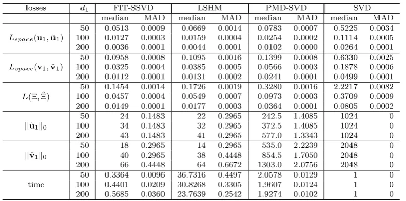
1.1 Comparison of four methods in the rank-one case: u1 is wc-peak, v1 is wc-poly, and the noise is iid N(0,1). . . 20

1.2 Comparison of four methods in the rank-one case: u1 is wc-peak, v1 is wc-poly, and the noise is iid

√

3/5t₅. . . 23

1.3 Comparison of four methods for the rank-two case, and the noise is iidN(0,1). . . 25 1.4 Mortality data: number of nonzero coordinates in the transformed

domain for four methods. . . 27 1.5 Cancer data: summary of cardinality of joint support of three

sin-gular vectors for four methods. . . 31

(11)

LIST OF FIGURES

1.1 (a) peak: three-peak function evaluated at 1024 equispaced loca-tions; (b)poly: piecewise polynomial function evaluated at 2048 eq-uispaced locations; (c)wc-peak: discrete wavelet transform (DWT) of the three-peak function; (d) wc-poly: DWT of the piecewise polynomial function. In Plot (c) and (d), each vertical bar is pro-portional in length to the magnitude of theSymmlet 8 wavelet co-efficient at the given location and resolution level. . . 20 1.2 (a)step: step function evaluated at 1024 equispaced locations, (b)sing:

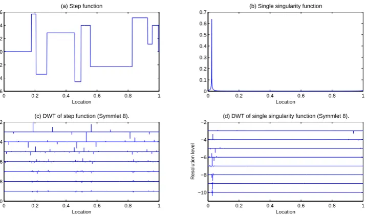
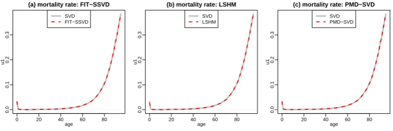
single singularity function evaluated at 2048 equispaced locations, (c)wc-step: DWT of step function, (d)wc-sing: DWT of single singularity function. . . 24 1.3 Mortality data: plot of ˆu1. Panel (a): FIT-SSVD vs. SVD; Panel

(b): LSHM vs. SVD; Panel (c): PMD-SVD vs. SVD. . . 27 1.4 Mortality data: Plot of ˆu1. Zoom of the lower left corner of Figure

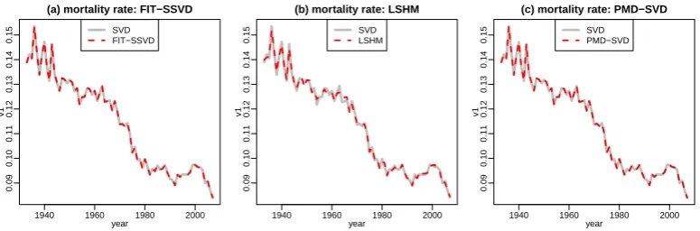
1.3. Everything else is the same as in Figure 1.3. . . 28 1.5 Mortality data: Plot of ˆv1. Everything else is the same as in

Fig-ure 1.3. . . 28 1.6 Mortality data: plot of ˆu2. Everything else is the same as Figure 1.3. 29

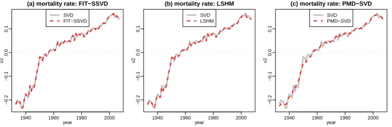
1.7 Mortality data: plot of ˆv2. Everything else is the same as Figure 1.3. 29

1.8 Cancer data: Scatterplots of the entries of the first three right singu-lar vectors ˆvl, l= 1,2,3 for four methods. Points represent patients.

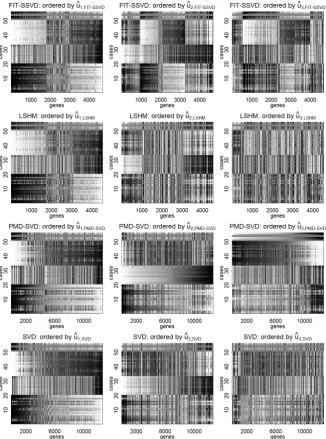
Black circle: Carcinoid; Red triangle: Colon; Green cross: Normal; Blue diamond: SmallCell. . . 33 1.9 Cancer data: Image plots of the rank-three approximationsP

l=1,2,3dˆluˆlvˆ

0

l

whose values are gray-coded. Each image is laid out as cases (= rows) by genes (= columns). The same rank-three approximation is shown three times for each method (left to right), each time sorted accord-ing to a different ˆul (l = 1,2,3). (The mapping of the rank-three

(12)

CHAPTER 1 METHODOLOGY

1.1 Introduction

Singular value decompositions (SVD) and principle component analyses (PCA)

are the foundations for many applications of multivariate analysis. They can be

used for dimension reduction, data visualization, data compression and

informa-tion extracinforma-tion by extracting the first few singular vectors or eigenvectors; see,

for example, Alter et al. (2001), Prasantha et al. (2007), Huang et al. (2009),

Thomasian et al. (1998). In recent years, the demands on multivariate methods

have escalated as the dimensionality of data sets has grown rapidly in such fields

as genomics, imaging, financial markets. A critical issue that has arisen in large

datasets is that in very high dimensional settings classical SVD and PCA can have

poor statistical properties (Shabalin and Nobel 2010, Nadler 2009, Paul 2007, and

Johnstone and Lu 2009). The reason is that in such situations the noise can

over-whelm the signal to such an extent that traditional estimates of SVD and PCA

(13)

there-fore be entirely misleading. Compounding the problems in large datasets are the

difficulties of computing numerically precise SVD or PCA solutions at affordable

cost. Obtaining statistically viable estimates of eigenvectors and eigenspaces for

PCA on high-dimensional data has been the focus of a considerable literature; a

representative but incomplete list of references is Lu (2002), Zou et al. (2006),

Paul (2007), Paul and Johnstone (2007), Shen and Huang (2008), Johnstone and

Lu (2009), Shen et al. (2011), Ma (2011). On the other hand, overcoming similar

problems for the classical SVD has been the subject of far less work, pertinent

articles being Witten et al. (2009), Lee et al. (2010a), Huang et al. (2009) and

Allen et al. (2011).

In the high dimensional setting, statistical estimation is not possible without

the assumption of strong structure in the data. This is the case for vector data

un-der Gaussian sequence models (Johnstone, 2011), but even more so for matrix data

which require assumptions such as low rank in addition to sparsity or smoothness.

Of the latter two, sparsity has slightly greater generality because certain types of

smoothness can be reduced to sparsity through suitable basis changes (Johnstone,

2011). By imposing sparseness on singular vectors, one may be able to “sharpen”

the structure in data and thereby expose “checkerboard” patterns that convey

biclustering structure, that is, joint clustering in the row- and column-domains of

the data (Lee et al. 2010a and Sill et al. 2011). Going one step further, Witten and

Tibshirani (2010) used sparsity to develop a novel form of hierarchical clustering.

So far we implied rather than explained that SVD and PCA approaches are

not identical. Their commonality is that both apply to data that have the form

of a data matrix X = (xij) of size n × p. The main distinction is that the

(14)

multivariate distribution, whereas the SVD model assumes the rows i= 1,2, ..., n

to correspond to a “fixed effects” domain such as space, time, genes, age groups,

cohorts, political entities, industry sectors, ... . This domain is expected to have

near-neighbor or grouping structure that will be reflected in the observations xij

in terms of smoothness or clustering as a function of the row domain. In practice,

the applicability of either approach is often a point of debate (e.g., should a set

of firms be treated as a random sample of a larger domain or do they constitute

an enumeration of the domain of interest?), but in terms of practical results the

analyses are often interchangeable because the points of difference between the

SVD and PCA models are immaterial in the exploratory use of these techniques.

The main difference between the models is that the SVD approach analyzes the

matrix entries as structuredlow-rank means plus error, whereas the PCA approach

analyzes the covariation between the column variables.

In modern developments of PCA, interest is focused on “functional” data

anal-ysis situations or on the analog of the “sequence model” (Johnstone, 2011) where

the columns also correspond to a structured domain such as space, time, genes, ... .

It is only with this focus that notions of smoothness and sparseness in the column

or row domain are meaningful. A consequence of this focus is the assumption that

all entries in the data matrix have the same measurement scale and unit, unlike

classical PCA where the columns can correspond to arbitrary quantitative

vari-ables with any mix of units. With identical measurement scales throughout the

data matrix, it is meaningful to entertain decompositions of the data into signal

and fully exchangeable noise:

X = Ξ +Z , (1.1)

(15)

an n×p random matrix representing the noise and consisting of i.i.d. errors as

its components. In both PCA and SVD approaches, the signal is assumed to

have a multiplicative low-rank structure: Ξ = U DV0 = Pr

l=1dlulv

0

l, where for

identifiability it is assumed that rank r < min(n, p), usually even “” such as

r= 1, 2 or 3. The difference between SVD and PCA is, using ANOVA language,

that in the SVD approach both U and V represent fixed effects that can both be

regularized with smoothness or sparsity assumptions, whereas in functional PCA

U is a random effect. As indicated above, such regularization is necessary for large

nandpbecause for realistic signal-to-noise ratios recovery of the trueU andV may

not be possible. — Operationally, estimation under sparsity is achieved through

thresholding. In general, if both matrix dimensions are thresholded, one obtains

sparse singular vectors of X; if only the second matrix dimension is thresholded,

one obtains sparse eigenvectors of X0X, which amounts to sparse PCA.

A few recent papers propose sparsity approaches to the high dimensional SVD

problem: Witten et al. (2009) introduced a matrix decomposition which constrains

the l1 norm of the singular vectors to impose sparsity on the solutions. Lee et al.

(2010a) used penalized LS for rank-one matrix approximations with l1 norms of

the singular vectors as additive penalties. Both methods use iterative procedures

to solve different optimization problems. [We will give more details about these

two methods in Section 1.3.] Allen et al. (2011) is a Lagrangian version of Witten

et al. (2009) where the errors are permitted to have a known type of dependence

and/or heteroscedasticity. These articles focus on estimating the first rank-one

term given by ˆd1,uˆ1,vˆ1 by either constraining the l1 norm of ˆu1 and ˆv1 or adding

it as a penalty. To estimate ˆd2,uˆ2,vˆ2 for a second rank-one term, they subtract

the first term ˆd1uˆ1vˆ01 from the data matrix X and repeat the procedure on the

(16)

for example, by Zheng et al. (2007), Mairal et al. (2010) and Bach et al. (2008),

but these do not have the form of a SVD. In our simulations and data examples we

use the proposals by Witten et al. (2009) and Lee et al. (2010a) for comparison.

Our approach is to estimate the subspaces spanned by the leading singular

vectors simultaneously. As a result, our method yields sparse singular vectors

that are orthogonal, unlike the proposals by Witten et al. (2009) and Lee et al.

(2010a). In terms of statistical performance, simulations show that our method

is competitive with the better performing of the two proposals, which is generally

Lee et al. (2010a). In terms of computational speed, our method is faster by at

least a factor of two compared to the more efficient of the two proposals, which

is generally Witten et al. (2009). Thus we show that the current state of the

art in sparse SVDs is “inadmissible” if measured by the two metrics ‘statistical

performance’ and ‘computational speed’: our method closely matches the better

statistical performance and provides it at a fraction of the better computational

performance. In fact, by making use of sparsity at the initialization stage, our

method also beats the conventional SVD in terms of speed.

Lastly, our method is grounded in asymptotic theory that comprises minimax

results which we describe in Chapter 2. A signature of this theory is that it is not

concerned with optimization problems but with a class of iterative algorithms that

form the basis of the methodology proposed here. As do most asymptotic theories

in this area, ours relies heavily on Gaussianity of noise, which is the major aspect

that needs robustification when turning theory into methodology with a claim to

practical applicability. Essential aspects of our proposal therefore relate to lesser

reliance on the Gaussian assumption.

(17)

for computing sparse SVDs. Section 1.3 shows simulation results to compare the

performance of our method with that of Witten et al. (2009) and Lee et al. (2010a).

Section 1.4 applies our and the competing methods to real data examples. Finally,

Section 1.5 discusses the results and open problems.

1.2 Methodology

In this section, we give a detailed description of the proposed sparse SVD method.

To start, consider the noiseless case. Our sparse SVD procedure is motivated

by the simultaneous orthogonal iteration algorithm (Golub and Van Loan 1996,

Chapter 8), which is a straightforward generalization of the power method for

computing higher-dimensional invariant subspaces of symmetric matrices. For an

arbitrary rectangular matrix Ξ of size n×p with SVD Ξ = U DV0, one can find

the subspaces spanned by the first r (1 ≤ r ≤ min(n, p)) left and right singular

vectors by iterating the pair of mappings V 7→ U and U 7→ V with Ξ and Ξ0 (its

transpose), respectively, each followed by orthnormalization, until convergence.

More precisely, given a right starting frame V(0), that is, a p×r matrix with r

orthonormal columns, the SVD subspace iterations repeat the following four steps

until convergence:

(1) Right-to-Left Multiplication: U(k),mul = ΞV(k−1)

(2) Left Orthonormalization with QR Decomposition: U(k)R(uk) =U(k),mul

(3) Left-to-Right Multiplication: V(k),mul = Ξ0U(k)

(4) Right Orthonormalization with QR Decomposition: V(k)_R(k)

v =V(k),mul

(1.2)

(18)

intermediate result of multiplication. For r = 1, the QR decomposition step

re-duces to normalization. If Ξ is symmetric, the second pair of steps is the same

as the first pair, hence the original orthogonal iteration algorithm for symmetric

matrices is a special case of the above algorithm.

The problems our approach addresses are the following: For large noisy

ma-trices in which the significant structure is concentrated in a small subset of the

matrix X, the classical algorithm outlined above produces estimates with large

variance due to the accumulation of noise from the majority of structureless cells

(Shabalin and Nobel, 2010). In addition to the detriment for statistical estimation,

involving large numbers of structureless cells in the calculations adds unnecessary

computational cost to the algorithm. Thus, shaving off cells with little apparent

structure has the promise of both statistical and computational benefits. This is

indeed borne out in the following proposal for a sparse SVD algorithm.

1.2.1 The FIT-SSVD Algorithm:

“Fast Iterative Thresholding for Sparse SVDs”

Unsurprisingly, the algorithm to be proposed here involves some form of

thresh-olding, be it soft or hard or something inbetween. All thresholding schemes reduce

small coordinates in the singular vectors to zero, and additionally such schemes

may or may not shrink large coordinates as well. Any thresholding reduces

vari-ance at the cost of some bias, but if the sparsity assumption is not too

unreal-istic, the variance reduction will vastly outweigh the bias inflation. The obvious

places for inserting thresholding steps are right after the multiplication steps. If

thresholding reduces a majority of entries to zero, the computational cost for the

(19)

Input:

1. Observed data matrix X. 2. Target rank r.

3. Thresholding function η.

4. Initial orthonormal matrix V(0) _∈

Rp×r.

5. Algorithm f to calculate the threshold level γ=f(X, U, V,σˆ) given (a) the data matrix X, (b) current estimates of left and right singular vectors U, V, and (c) an estimate of the standard deviation of noise ˆσ. (Algorithm 3 is one choice.)

Output: Estimators ˆU =U(∞) and ˆV =V(∞). 1 Set ˆσ= 1.4826 MAD (as.vector(X)).

repeat

2 Right-to-Left Multiplication: U(k),mul =XV(k−1). 3 Left Thresholding: U(k),thr = (u_il(k),thr), withu(_ilk),thr =η

u(_ilk),mul, γul

, where γu =f(X, U(k−1), V(k−1),σˆ).

4 Left Orthonormalization with QR Decomposition: U(k)Ru(k)=U(k),thr.

5 Left-to-Right Multiplication: V(k),mul =X0U(k).

6 Right Thresholding: V(k),thr = (v_jl(k),thr), withv_jl(k),thr =η

v(_jlk),mul, γvl

, where γv =f(X0, V(k−1), U(k),σˆ).

7 Right Orthonormalization with QR Decomposition: V(k)Rv(k)=V(k),thr.

until Convergence;

Algorithm 1: FIT-SSVD

The iterative procedure we propose is schematically laid out in Algorithm 1.

In what follows we discuss the thresholding function and convergence criterion

of Algorithm 1. Subsequently, in Sections 1.2.2–1.2.4, we describe other important

aspects of the algorithm: the initialization of the orthonormal matrix, the target

rank, and the adaptive choice of threshold levels.

Thresholding function At each thresholding step, we perform entry-wise

olding. In our modification of the subspace iterations (1.2) we allow any

thresh-olding function η(x, γ) that satisfies|η(x, γ)−x| ≤γ and η(x, γ)1|x|≤γ = 0, which

(20)

withηhard(x, γ) =x1|x|>γ, as well as the thresholding function used in SCAD (Fan

and Li, 2001). The parameter γ is called the threshold level. In Algorithm 1, we

apply the same threshold levelγul (or γvl) to all the elements in thelth column of

U(k),mul _(or_V(k),mul_{, resp.). For more details on threshold levels, see Section 1.2.4.}

Convergence criterion We stop the iterations once subsequent updates of the

orthonormal matrices are very close to each other. In particular, for any

ma-trix H with orthonormal columns (that is, H0H = I), let PH = HH0 be the

associated projection matrix. We stop after the kth iteration if max{kP_U(k) −

P_U(k−1)k2₂,kP_V(k)−P_V(k−1)k2₂} ≤, whereis a pre-specified tolerance level, chosen

to be = 10−8 for the rest of this chapter. [kAk2 denotes the spectral norm ofA.]

1.2.2 Initialization algorithm for FIT-SSVD

In Algorithm 1, we need a starting frame V(0) _{such that the subspace it spans has}

no dimension that is orthogonal to the subspace spanned by the true V. Most

often used is the V frame provided by the ordinary SVD. However, due to its

denseness, computational cost and inconsistency (Shabalin and Nobel, 2010), it

makes an inferior starting frame. Another popular choice is initialization with a

random frame, which, however, is often nearly orthogonal to the trueV and thus

requires many iterations to accumulate sufficient power to converge. We propose

therefore Algorithm 2 which overcomes these difficulties.

The algorithm is motivated by Johnstone and Lu (2009) who obtained a

con-sistent estimate for principal components under a sparsity assumption by initially

reducing the dimensionality. We adapt their scheme to the two-way case, and we

(21)

Input:

1. Observed data matrix X. 2. Target rank r.

3. Degree of “Huberization” β (typically 0.95 or 0.99),

that defines a quantile of the absolute values of entries in X. 4. Significance level of a selection test α.

Output: Orthornormal matrices ˆU =U(0) and ˆV =V(0).

1 Subset selection:

Let δ be the β-quantile of the absolute values of all the entries in X. Define Y = (yij) by yij =ρ(xij, δ), where ρ(x, δ) is the Huber ρ function:

ρ(x, δ) = x2 _if _|_x_{| ≤}_δ _{and 2}_δ_|_x_{| −}_δ2 _otherwise.

Select a subset I ={i1, i2, ...} of rows according to the next four steps:

− Let ti =

Pp

j=1yij fori= 1, . . . , n.

− Let ˆµ= median(t1, ..., tn) and ˆs= 1.4826 MAD(t1, ..., tn).

− Calculate p-values: pi = 1−Φ(ti−_ˆ_sµˆ), where Φ is the CDF of N(0,1).

− Perform the Holm method on the p-values at family-wise error rate α, and letI be the indices of the p-values that result in rejection.

Select a subset of columns J similarly. Form the submatrix XIJ of size |I| × |J|.

2 Reduced SVD: Compute r leading pairs of singular vectors of the submatrix

XIJ.

Denote them by uI₁, . . . ,uI_r (|I| ×1 each) and v₁J, . . . ,v_rJ (|J| ×1 each). 3 Zero-padding: Create U(0) = [u(0)₁ , . . . ,u(0)r ] (n×r) and

V(0) _{= [}_v(0)

1 , . . . ,v (0)

r ] (p×r),

such that u(0)_Il =uI Il, u

(0)

Ic_l = 0, v

(0)

J l =vJJ l, v (0) Jc_l= 0.

Algorithm 2: Initialization algorithm for FIT-SSVD.

result in too great a sensitivity to even slightly heavier tails than normal. To this

end we make use of some devices from robust estimation. The intent is to perform

a row- and column-preselection (Step 1) before applying a classical SVD (Step 2)

so as to concentrate on a much smaller submatrix that contains much of the signal.

We discuss the row selection process, column selection being analogous.

Signal strength in rows would conventionally be measured under Gaussian

as-sumptions with row sums of squares and tested with χ2 _{tests with} _p _{degrees of}

freedom. As mentioned this approach turns out to be much too sensitive when

(22)

than normal tails. We therefore mute the influence of isolated large cells by

Hu-berizing the squares before forming row sums. We then form approximatez-score

test statistics, one per row, drawing on the CLT since we assumep(the number of

entries in each row) to be large. Location and scale for thez-scores are estimated

with the median and MAD (“median absolute deviation”, instead of mean and

standard deviation) of the row sums, the assumption being that over half of the

rows are approximate “null rows” with little or no signal. If the signal is not sparse

in terms of rows, this procedure will have low power, which is desirable because

it biases the initialization of the iterative Algorithm 1 toward sparsity. Using

ro-bust z-score tests has two benefits overχ2 tests: they are robust to isolated large

values, and they avoid the sensitivity of χ2 _{tests caused by their rigid coupling of}

expectation and variance. Finally, since n tests are being performed, we protect

against over-detection due to multiple testing by applying Holm’s (1979) stepwise

testing procedure at a specified family-wise significance levelα(default: 5%). The

end result are a set of indices I of “significant rows”. — The same procedure is

then applied to the columns, resulting in an index setJ of “significant columns”.

The submatrixXIJ is then submitted to an initial reduced SVD. It is this initial

reduction that allows the present algorithm to be faster than a conventional SVD

of the full matrix X when the signal is sparse. The left and right singular vectors

are of size |I| and |J|, respectively. To serve as initializations for the iterative

Algorithm 1, they are expanded and zero-padded to length n and p, respectively

(23)

1.2.3 Rank estimation

In Algorithm 1, a required input is the presumed rank of the signal underlying

X. In practice, we need to determine the rank based on the data. Proposals for

rank estimation are the subject of a literature with a long history, of which we

only cite Wold (1978), Gabriel (2002), and Hoff (2007). The proposal we chose

is the bi-cross-validation (BCV) method by Owen and Perry (2009), but with a

necessary twist.

The original BCV method was proposed for low-rank matrices with dense

singular vectors. Thus, we apply it to the submatrix XIJ obtained from the

initialization Algorithm 2, instead of X itself. The submatrix should have much

denser singular vectors and, even more importantly, much higher signal to noise

ratio compared to the full matrix. In simulations not reported here but similar

to those of Section 1.3, BCV on XIJ yielded consistent rank estimation when the

signal was sufficiently strong for detection in relation to sparsity and

signal-to-noise ratio.

1.2.4 Threshold levels

The tuning parameters γ in the thresholding function η(x, γ) are called

“thresh-old levels”; they play a key role in the procedure. At each thresh“thresh-olding step in

Algorithm 1, a (potentially different) threshold level needs to be chosen for each

column l = 1, ..., r of U(k) _and _V(k) _{to strike an acceptable bias-variance}

trade-off. In what follows, we focus on U(k)_{, while the case of} _V(k) _{can be obtained by}

(24)

The goal is to process the iterating left and right frames in such a way as

to retain the coordinates with high signal and eliminate those with low signal.

To be more specific, we focus on one column u(_lk),mul = Xv(_lk−1). Recall that X

is assumed to admit an additive decomposition into a low-rank signal plus noise

according to model (1.1). Then a theoretically sensible (though not actionable)

threshold level foru(_lk),mul would beγul = E[kZv

(k−1)

l k∞], where Z is the additive

noise matrix, and kZv_l(k−1)k∞ is the maximum absolute value of the n entries in

the vector Zv(_lk−1). The signal of any coordinate in u(_lk),mul with value less than

γul could be regarded low since it is weaker than the expected maximum noise

level in the l’th rank given that there are n rows.

The threshold γul as written above is of course not actionable because it

in-volves knowledge of Z, but we can obtain information by leveraging the

(presum-ably large) part ofX that is estimated to have no or little signal. This can be done

as follows: Let Lu be the index set of rows which have all zero entries in U(k−1),

and letHu be its complement; define Lv and Hv analogously. We may think ofLu

and Lv as the current estimates of low signal rows and columns. Consider next

a reordering and partitioning of the rows and columns of X according to these

index sets:

X =



 

XHuHv XHuLv

XLuHv XLuLv





. (1.3)

Since the entries in v(_lk−1) corresponding to Lv are zero, only X:Hv (of size n×

|Hv|, containing the two left blocks in (1.3)) is effectively used in the right-to-left

multiplication of the iterative Algorithm 1. We can therefore simulate a

“near-null” situation in this block by filling it with random samples from the bottom

(25)

Denote the result of such “bootstrap transfer” fromXLuLvtoX:Hv by ˜Z

∗₍_n_×|_H

v|).

Passing ˜Z∗ through the right-to-left multiplication with v(_lk−1) we form Z∗v(_Hk_v−_l1),

which we interpret as an approximate draw from Zv_l(k−1). We thus estimate

kZv(_lk−1)k∞ with kZ∗v

(k−1)

Hvl k∞, and E[kZv

(k−1)

l k∞] with a median of kZ

∗_v(k−1) Hvl k∞

over multiple bootstraps of Z∗.

In order for this to be valid, the block XLuLv needs to be sufficiently large in

relation toX:Hv. This is the general problem of the “mout ofn” bootstrap, which

was examined by Bickel et al. (1997). According to their results, this bootstrap is

generally consistent as long asm =o(n). Hence, when the size|Lu||Lv|of the

ma-trix XLuLv is large, say, larger than n|Hv|log(n|Hv|), we estimate E[kZv

(k−1)

1 k∞]

by the median of M bootstrap replications for sufficiently large M. When the

condition is violated,|Hv|tends to be large, the central limit theorem takes effect,

and each element of Zv₁(k−1) would be close to a normal random variable. Thus,

the expected value of the maximum is near the asymptotic value √2 logn times

the standard deviation. — We have now fully defined the thresholdγul to be used

onu(_lk),mul. The thresholds forl = 1, ..., r are then collected in the threshold vector

γu = (γu1, ..., γur)0.

A complete description of the scheme is given in Algorithm 3. Based on an

extensive simulation study, setting the number of bootstrap replications to M =

100 yields a good balance between the accuracy of the threshold level estimates

(26)

Input:

1. Observed data matrix X ∈_Rn×p_;

2. Previous estimators of singular vectors U(k)∈_Rn×r_,_V(k) _∈

Rp×r; 3. Pre-specified number M of bootstraps;

4. Estimate of the standard deviation of noise ˆσ.

Output: Threshold levelγ ∈_Rr_.

1 Subset selection: Lu ={i:u_i(₁k) =...=u(_irk) = 0},

Lv ={j :v(_jk₁) =...=v_jr(k) = 0},

Hu =Lcu, Hv =Lcv;

2 if |L_v||L_u|< n|H_v|log(n|H_v|) then

3 return γ = ˆσp2 log(n)1∈_Rr ;

else

4 for i←1 to M do

5 Sample n|H_v| entries from X_L_u_L_v and reshape them into a matrix ˜

Z ∈_Rn×|Hv|_;

6 B = ˜ZV_H(k)

v:∈R

n×r_;

7 C_i_:= (kB_:1k∞,kB:2k∞, . . . ,kB:rk∞)0; 8 γ_l = median(C_:_l);

9 return γ = (γ₁, ..., γ_r)0.

Algorithm 3:The threshold level functionf(X, U, V,σˆ) for Algorithm 1. As

shown, the code produces thresholds for U. A call to f(X0, V, U,σˆ) produces thresholds for V.

1.2.5 Alternative methods for selecting threshold levels

In methods for sparse data, one of the most critical issues is selecting threshold

levels wisely. Choosing thresholds too small kills off too few entries and retains

too much variance, whereas choosing them too large kills off too many entries and

introduces too much bias. To navigate this bias-variance trade-off, we adopted in

Section 1.2.4 an approach that can be described as a form of testing: we established

max-thresholds that are unlikely to be exceeded by anyU- orV-coordinates under

the null assumption of absent signal in the corresponding row or column of the

data matrix.

(27)

various forms of cross-validation, a version of which we adopted for the different

problem of rank selection in Section 1.2.3 (bi-cross-validation or BCV according

to Owen and Perry (2009)). Indeed, a version of cross-validation for threshold

selection is used by one of the two competing proposals with which we compare

ours: Witten et al. (2009) leave out random subsets of the entries in the data

matrix, measure the differences between the fitted values and the original values

for those entries, and choose the threshold levels that minimize the differences.

Alternatively one could use bi-cross-validation (BCV) for this purpose as well, by

leaving out sets of rows and columns and choosing the thresholds that minimize

the discrepancy between the hold-out and the predicted values. However, this

would be computationally slow for simultaneous minimization of two threshold

parameters. Moreover, the possible values of the thresholds vary from zero to

infinity, which makes it difficult to choose grid points for the parameters. In order

to avoid such issues, Lee et al. (2010a) implement their algorithm by embedding

the optimization of the choice of the threshold level inside the iterations that

calculate ul for fixed vl and vl for fixed ul (unlike our methods, theirs fits one

rank at a time). They minimize a BIC criterion over a grid of order statistics of

current estimates. This idea could be applied to our simultaneous space-fitting

approach, but the simulation results in Section 1.3 below show that the method

of Lee et al. (2010a) is computationally very slow.

1.3 Simulation results

In this section, we show the results of numerical experiments to compare the

performance of FIT-SSVD with two state-of-the-art sparse SVD methods from

(28)

acquires whole subspaces spanned by sparse vectors simultaneously, both

compari-son methods are stepwise procedures that acquire sparse rank-one approximations ˆ

dluˆlvˆl0 successively; for example, the second rank-one approximation ˆd2u2ˆ vˆ02 is

found by applying the same method to the residual matrix X −dˆ1uˆ1vˆ01, and so

on. For both methods it is therefore only necessary to describe how they obtain

the first rank-one term.

• The first sparse SVD algorithm for comparison was proposed by Lee et al.

(2010a) [referred to from here on by their initials, “LSHM”]. They obtain a

first pair of sparse singular vectors by finding the solution to the following

l1 penalized SVD problem under an l2 constraint:

min

u,v,s kX−suv

0_k2

F +sλukuk1+sλvkvk1

. subject to kuk2 =kvk2 = 1.

LSHM solve this problem by alternating between the following steps till

convergence:

(1) u˜l =ηsof t(Xvlold, λu), unewl ← ˜

ul

ku˜lk2 ,

(2) v˜l =ηsof t(X0unewl , λv), vnewl ← ˜

vl

kv˜lk2 .

• The second sparse SVD algorithm for comparison with our proposal is the

adaptation of the penalized matrix decomposition scheme by Witten et al.

(2009) to the sparse SVD case [referred to as “PMD-SVD” from here on].

They obtain the first pair of sparse singular vectors by imposing simultaneous

l1 and l2 constraints on both vectors:

(29)

The PMD-SVD algorithm iterates between the following two steps until

convergence:

(1) u= ηsof t(Xv, δu)

kηsof t(Xv, δu)k2 ,

where δu is chosen by binary search such that kuk1 =su,

(2) v= ηsof t(X 0_u_{, δ}

v)

kηsof t(X0u, δv)k2 ,

where δv is chosen by binary search such that kvk1 =sv.

To make fair comparisons, we use the implementations by their original authors

for both LSHM (Lee et al., 2010b) and PMD-SVD (Witten et al., 2010). The

tuning parameters are always chosen automatically by the default methods in

their implementations. For FIT-SSVD, we always use η = ηhard in Algorithm 1,

Huberization β = 0.95 and Holm family-wise error rate α = 0.05 in Algorithm 2,

and M = 100 bootstraps in Algorithm 3. We did try different values of α, β and

M in FIT-SSVD, and the results are not sensitive to these choices. Thus, in our

experience there is no need for cross-validated selection of these parameters.

In what follows, we report simulation results for situations in which the true

underlying matrix has rank one and two, respectively. Throughout this section,

the rank of the true underlying matrix is assumed known.

1.3.1 Rank-one results

In this part, we generate data matrices according to model (1.1) with rankr = 1,

n = 1024 and p = 2048, the singular value d1 ranging in {50,100,200}, and iid

noise Zij ∼ (µ=0, σ2=1). At first glance d1 = 50 may appear like an outsized

(30)

E[kZk2

F] =np ≈ 2 million, whereas the sum of squares of signal is a comparably

vanishingkd1u1v0₁k2

F =d21 = 2500, for a signal-to-noise ratioS/N = 0.0012 (which

makes the failure of the ordinary SVD in these tasks less surprising). Even d1 =

200 amounts to a S/N = 0.012 only.

As mentioned in the introduction, the FIT-SSVD method was motivated by

theoretical results that were based on Gaussian assumptions (Yang et al., 2011); it

is therefore a particular concern to check the robustness of the method under noise

with heavier tails than Gaussian. To this end we report simulation results both

forN(0,1) andp3/5t5 noise, the latter also having unit variance (the purpose of

the factorp3/5).

For the construction of meaningful singular vectors we use a functional data

analysis context: We choose functions gleaned from the literature and represent

them in wavelet bases where they feature realistic degrees of sparsity. In Figure 1.1,

Plot (a) (“peak”) shows the graph of a function with three peaks, evaluated at 1024 equispaced locations, while Plot (b) (“poly”) shows a piecewise polynomial function, evaluated at 2048 equispaced locations. Both functions create dense

evaluation vectors but sparse wavelet coefficient vectors. [In all simulation results

reported below, we use Symmelet 8 wavelet coefficients (Mallat, 2009).] Multi-resolution plots of the wavelet coefficients are shown in Plots (c) (“wc-peak”) and (d) (“wc-poly”) of Figure 1.1. We choose u1 and v1 to be the wavelet coefficient vectors wc-peakand wc-poly, respectively.

For each simulated scenarios, we ran 100 simulations, applied each algorithm

under comparison, and summarized the results in terms of median and

MAD-based standard error. The criteria which we use for comparison of the methods

(31)

0 0.2 0.4 0.6 0.8 1 0 0.05 0.1 0.15 0.2 0.25

(a) Three peak function

Location

0 0.2 0.4 0.6 0.8 1

−0.04 −0.02 0 0.02 0.04 0.06 0.08

(b) Piecewise polynomial function

Location

0 0.2 0.4 0.6 0.8 1

−10 −8 −6 −4 −2

(c) DWT of 3−peak function (Symmlet 8).

Location

Resolution level

0 0.2 0.4 0.6 0.8 1

−10 −8 −6 −4 −2

(d) DWT of piecewise polynomial function (Symmlet 8).

Location

Resolution level

Figure 1.1: (a) peak: three-peak function evaluated at 1024 equispaced loca-tions; (b)poly: piecewise polynomial function evaluated at 2048 equispaced loca-tions; (c)wc-peak: discrete wavelet transform (DWT) of the three-peak function; (d)wc-poly: DWT of the piecewise polynomial function. In Plot (c) and (d), each vertical bar is proportional in length to the magnitude of the Symmlet 8 wavelet coefficient at the given location and resolution level.

losses d1 FIT-SSVD LSHM PMD-SVD SVD

median MAD median MAD median MAD median MAD

Lspace(u1,uˆ1)

50 0.0513 0.0009 0.0669 0.0014 0.0783 0.0007 0.5225 0.0034

100 0.0127 0.0003 0.0159 0.0004 0.0254 0.0002 0.1114 0.0005

200 0.0036 0.0001 0.0044 0.0001 0.0102 0.0000 0.0264 0.0001

Lspace(v1,vˆ1)

50 0.0958 0.0008 0.1095 0.0016 0.1399 0.0008 0.6330 0.0025

100 0.0325 0.0004 0.0385 0.0005 0.0566 0.0003 0.1878 0.0006

200 0.0112 0.0001 0.0131 0.0002 0.0241 0.0001 0.0499 0.0001

L(Ξ,Ξ)ˆ

50 0.1454 0.0014 0.1726 0.0019 0.3280 0.0016 2.2217 0.0082

100 0.0457 0.0004 0.0549 0.0007 0.0973 0.0003 0.3709 0.0009

200 0.0149 0.0001 0.0177 0.0003 0.0364 0.0001 0.0805 0.0002

kuˆ1k0

50 24 0.1483 22 0.2965 242.5 1.4085 1024 0

100 34 0.1483 32 0.2965 372.5 1.4085 1024 0

200 43 0.1483 41 0.2965 577.0 1.3343 1024 0

kvˆ1k0

50 18 0.2965 14 0.2965 535.0 2.2239 2048 0

100 40 0.2965 38 0.4448 854.5 1.7050 2048 0

200 66 0.4448 64 0.6672 1303.0 2.0756 2048 0

time

50 0.3364 0.0096 36.7316 0.4497 2.0578 0.0129 1 0

100 0.4401 0.0209 30.8268 0.3305 1.9607 0.0124 1 0

200 0.5685 0.0360 23.7639 0.2542 1.9274 0.0102 1 0

Table 1.1: Comparison of four methods in the rank-one case: u1 iswc-peak,v1 is

(32)

N(0,1) noise Z:

• The first block examines the estimation accuracy of the left singular vector,

with the three rows corresponding to three different values of d1. Following

Ma (2011), we define the loss function for estimating the column space ofU

for a general rank-r byLspace(U,Uˆ) =kPU −P_Uˆk22 , wherePU =U U0 is the

projection matrix onto the subspace spanned by the columns ofU (which is

of sizen×r and has orthonormal columns, U0U =Ir). In the rank-one case

here, the loss reduces to sin2_∠(u1,uˆ1).

• The second block in Table 1.1 reports the loss for right singular vectors.

• The third block shows the scaled recovery error for the low-rank signal matrix

Ξ = U DV0, defined as L(Ξ,Ξ) =ˆ kΞˆ −Ξk2

F/kΞk2F. Here, ˆΞ = ˆUDˆVˆ

0 _and

ˆ

D=diag( ˆd1, . . . ,dˆr) with diagonal entries being ˆdl = ˆu0lXvˆl.

• The fourth and fifth panels of Table 1.1 show the sparsity of the solutions

measured by kuˆ1k0 and kvˆ1k0, that is, the number of nonzero elements in

the estimates.

• The last block shows timing results as a fraction or multiple of the ordinary

SVD.

The results are as follows:

• From the first three blocks we see that FIT-SSVD uniformly outperforms the

other methods with respect to the three statistical criteria. While LSHM

is not far behind FIT-SSVD, PMD-SVD lags in several cases by a factor

of two or more. The ordinary SVD fails entirely for low signal strength as

(33)

in such situations. Rather expectedly, all methods achieve better statistical

accuracy as the signal strength d1 increases

• As for the sparsity metrics, FIT-SSVD and LSHM produce similar levels

of sparsity, while PMD-SVD estimators are much denser. The results also

suggest that as the signal strength d1 gets stronger, the three sparse SVD

methods estimate more coordinates.

• Finally, the timing results indicate that FIT-SSVD is faster than all other

methods, the ordinary SVD included. LSHM stands out as slower than

FIT-SSVD by factors of over 40 to over 100. PMD-SVD is more competitive but

still at least a factor of three slower than FIT-SSVD. The variation in time

for PMD-SVD is small because the majority is spent in cross-validation.

To examine the effect of heavy-tailed noise, we report in Table 1.2 the

simula-tion results when the entries of the noise matrixZ are distributed iidp3/5t5, all

else being the same as in Table 1.1. [Recall that the scaling factor p3/5 is used

to ensure unit variance.] The statistical performance for all methods is worse than

in Table 1.1. In terms of the statistical metrics, the performances of FIT-SSVD

and LSHM are in a statistical dead heat, whereas PMD-SVD trails behind by as

much as a factor of two in the case of high signal strength,d1 = 200. Again,

FIT-SSVD and LSHM have comparable sparsities, whereas PMD-SVD is much denser.

In terms of computation time, again FIT-SSVD is uniformly fastest, followed by

PMD-SVD which trails by factors of over two to over five, and LSHM being orders

(34)

losses d1 FIT-SSVD LSHM PMD-SVD SVD

Lspace(u1,uˆ1)

50 0.0802 0.0015 0.0819 0.0017 0.0907 0.0011 0.5405 0.0037

100 0.0177 0.0003 0.0180 0.0004 0.0282 0.0003 0.1115 0.0006

200 0.0048 0.0001 0.0047 0.0001 0.0108 0.0001 0.0262 0.0002

Lspace(v1,vˆ1)

50 0.1193 0.0014 0.1191 0.0018 0.1560 0.0014 0.6432 0.0039

100 0.0451 0.0005 0.0415 0.0007 0.0601 0.0003 0.1870 0.0006

200 0.0145 0.0002 0.0137 0.0002 0.0249 0.0001 0.0498 0.0002

L(Ξ,Ξ)ˆ

50 0.1944 0.0024 0.1937 0.0028 0.3719 0.0028 2.2624 0.0107

100 0.0625 0.0007 0.0600 0.0009 0.1041 0.0005 0.3706 0.0011

200 0.0192 0.0002 0.0187 0.0002 0.0378 0.0001 0.0805 0.0002

kuˆ1k0

50 20 0.2965 21.5 0.3706 235.0 1.5567 1024 0

100 31 0.1483 33.0 0.2965 364.0 1.8532 1024 0

200 40 0.1483 41.0 0.2965 569.5 2.0015 1024 0

kvˆ1k0

50 13 0.1483 14.0 0.2965 526.0 2.0015 2048 0

100 31 0.2965 38.5 0.5189 841.5 2.1498 2048 0

200 56 0.2965 64.5 0.6672 1307.5 2.2980 2048 0

time

50 0.3714 0.0190 41.0695 0.9339 2.0826 0.0046 1 0

100 0.8072 0.0652 30.5216 0.3774 2.0187 0.0039 1 0

200 0.8238 0.0710 23.0527 0.2554 1.9520 0.0048 1 0

Table 1.2: Comparison of four methods in the rank-one case: u1 iswc-peak,v1 is

wc-poly, and the noise is iid √3/5t₅.

1.3.2 Rank-two results

We show next simulation results for data according to model (1.1) with r = 2,

and again n = 1024 and p= 2048. The singular values (d1, d2) range among the

pairs (100,50), (200,50), and (200,100). The singular vectors are u1 =wc-peak, v1 =wc-poly, u2 = wc-step, and v2 =wc-sing, the properties of the latter two

vectors being shown in Figure 1.2.

Table 1.3 reports the results from 100 repetitions when the noise is iidN(0,1).

In terms of statistical metrics, FIT-SSVD always outperforms LSHM though not

hugely. PMD-SVD does slightly better than FIT-SSVD forLspace(U,Uˆ), but much

worse for Lspace(V,Vˆ) and L(Ξ,Ξ).ˆ This is due to the special type of

cross-validation used in the package PMA: the parameters su, sv are set to be propor-tional to each other after being scaled according to the dimensionality, √n and

√

p, which essentially reduces the simultaneous cross-validation on two parameters

(35)

0 0.2 0.4 0.6 0.8 1 −0.06 −0.04 −0.02 0 0.02 0.04 0.06

(a) Step function

Location

0 0.2 0.4 0.6 0.8 1

0 0.1 0.2 0.3 0.4 0.5 0.6 0.7

(b) Single singularity function

Location

0 0.2 0.4 0.6 0.8 1

−10 −8 −6 −4 −2

(c) DWT of step function (Symmlet 8).

Location

Resolution level

0 0.2 0.4 0.6 0.8 1

−10 −8 −6 −4 −2

(d) DWT of single singularity function (Symmlet 8).

Location

Resolution level

Figure 1.2: (a)step: step function evaluated at 1024 equispaced locations, (b)sing: single singularity function evaluated at 2048 equispaced locations, (c)wc-step: DWT of step function, (d)wc-sing: DWT of single singularity func-tion.

and ˆv.

In terms of sparsity of the estimators, the fourth and fifth blocks show the

cardinality of the joint support of the estimated singular vectors, which indicate

that FIT-SSVD and LSHM are again about comparable, and PMD-SVD is much

denser as in the rank-one case. [We do not compare the losses and the l0 norms

for individual singular vectors because LSHM and PMD-SVD do not produce

orthogonal singular vectors.]

Finally, in terms of computation time, FIT-SSVD dominates again, and the

differences become somewhat more pronounced than in the rank-one case. In the

high signal scenario, d1 = 200 and d2 = 100, FIT-SSVD gets a boost because by

avoiding the costly bootstrap in Algorithm 3 because Condition 2 is satisfied and

the much cheaper normal approximation on Line 3 of Algorithm 3 can be used

(36)

losses d1 d2 FIT-SSVD LSHM PMD-SVD SVD

Lspace(U,Uˆ)

100 50 0.1163 0.0010 0.1413 0.0021 0.1022 0.0009 0.5315 0.0037

200 50 0.1148 0.0013 0.1422 0.0018 0.1007 0.0009 0.5265 0.0027

200 100 0.0376 0.0003 0.0443 0.0006 0.0321 0.0003 0.1114 0.0005

Lspace(V,Vˆ)

100 50 0.0514 0.0009 0.0596 0.0010 0.1230 0.0008 0.6376 0.0029

200 50 0.0506 0.0009 0.0601 0.0011 0.1259 0.0006 0.6293 0.0023

200 100 0.0144 0.0002 0.0172 0.0003 0.0538 0.0002 0.1870 0.0005

L(Ξ,Ξ)ˆ

100 50 0.0691 0.0006 0.0825 0.0007 0.1403 0.0004 0.7439 0.0017

200 50 0.0234 0.0001 0.0285 0.0002 0.0529 0.0001 0.2070 0.0005

200 100 0.0228 0.0001 0.0261 0.0002 0.0483 0.0001 0.1387 0.0003

| ∪2

1supp(ˆul)|

100 50 49 0.2965 45.0 0.4448 479 1.1861 1024 0

200 50 56 0.2965 49.0 0.2965 649 1.5567 1024 0

200 100 77 0.2965 73.5 0.5189 657 1.3343 1024 0

| ∪2

1supp(ˆvl)|

100 50 54 0.2965 50.5 0.3706 1158.0 2.2239 2048 0

200 50 78 0.2965 74.5 0.5189 1486.5 2.1498 2048 0

200 100 81 0.4448 82.5 0.5930 1623.0 2.1498 2048 0

time

100 50 1.1675 0.0829 64.7840 0.6037 2.7991 0.0141 1 0

200 50 1.4572 0.1011 55.6839 0.5436 2.7018 0.0142 1 0

200 100 0.8000 0.0668 54.2361 0.2363 2.6429 0.0073 1 0

Table 1.3: Comparison of four methods for the rank-two case, and the noise is iidN(0,1).

matrix to get the second layer of SVD, computation time doubles. As for

PMD-SVD, since the time is mainly spent in cross-validation and the same penalty

parameter is used for different ranks, the increase in time is not obvious.

1.4 Real data examples

All the methods mentioned above require sparse singular vectors (with most entries

close to zero). One source of such data is two-way functional data whose row and

column domains are both structured, for example, temporally or spatially, as

when the data are time series collected at different locations in space. Two-way

functional data are usually smooth as functions of the row and column domains.

Thus, if we expand them in suitable basis functions, such as an orthonormal

(37)

1.4.1 Mortality rate data

As our first example we use the US mortality rate data from the Berkeley Human

Mortality Database (http://www.mortality.org/). They contain mortality rates

in the United States for ages 0 to 110 from 1933 to 2007. The data for people

older than 95 was discarded because of their noisy nature. The matrixX is of size

96×75, each row corresponding to an age group and each column to a one-year

period. We first pre- and post- multiply the data matrix with orthogonal matrices

whose columns are the eigenvectors of second order difference matrices of proper

sizes; the result is a matrix of coefficients of the same size as X. The rank of

the signal is estimated to be 2 using bi-crossvalidation (Section 1.2.3). We then

applied FIT-SSVD, LSHM, PMD-SVD and ordinary SVD to get the first two pairs

of singular vectors. Finally, we transformed the sparse estimators of the singular

vectors back to the original basis to get smooth singular vectors.

The estimated number of nonzero elements in each singular vector (before the

back transformation) is summarized in Table 1.4: none gives very sparse solutions.

This is reasonable, because the mortality rate data is of low noise and for data

with no noise we should just use the ordinary SVD. Because this data is of small

size, it only takes a few seconds for all the algorithms. The plot of singular vectors

for all the methods are shown in Figures 1.3 to 1.7. The red dashed line in the left

plot is for FIT-SSVD, in the middle for LSHM, and on the right for PMD-SVD.

We use the wider gray curve for the ordinary SVD as a reference.

Figure 1.3 shows the first left singular vector plotted against age. The curve

ˆ

u1 shows a pattern for mortality as a function of age: a sharp drop between age

(38)

FIT-SSVD LSHM PMD-SVD SVD

kuˆ1k0 82 48 96 96

ku2ˆ k0 86 56 7 96

kvˆ1k0 66 45 75 75

kvˆ2k0 70 45 43 75

Table 1.4: Mortality data: number of nonzero coordinates in the transformed domain for four methods.

begins an exponential increase. Figure 1.4 zooms into the lower left corner of

Figure 1.3 to show the details between age 0 and 10. LSHM, as always turns

out to be the sparsest (or smoothest) among the three iterative procedures in

the transformed (or original) domain. We believe that FIT-SSVD and PMD-SVD

make more sense based on a parallel coordinates plot of the raw data (not shown

here), in which the drop in the early age appears to be sharp and therefore should

not be smoothed out. Figure 1.5 shows the first right singular vectors plotted

against year. It implies that mortality decreases with time. All of the panels show

a wiggly structure, with LSHM again being the smoothest. Here, too, we believe

that the zigzag structure is real and not due to noise in the raw data, based again

on a parallel coordinate plot of the raw data. The zigzags may well be systematic

artifacts, but they are unlikely to be noise.

0 20 40 60 80

0.0

0.1

0.2

0.3

(a) mortality rate: FIT−SSVD

age

u1

SVD FIT−SSVD

0 20 40 60 80

0.0

0.1

0.2

0.3

(b) mortality rate: LSHM

age

u1

SVD LSHM

0 20 40 60 80

0.0

0.1

0.2

0.3

(c) mortality rate: PMD−SVD

age

u1

SVD PMD−SVD

Figure 1.3: Mortality data: plot of ˆu1. Panel (a): FIT-SSVD vs. SVD; Panel (b):

LSHM vs. SVD; Panel (c): PMD-SVD vs. SVD.

(39)

0 2 4 6 8 10

0.000

0.010

0.020

0.030

age

u1, z

oom

SVD FIT−SSVD

0 2 4 6 8 10

0.000

0.010

0.020

0.030

age

u1, z

oom

SVD LSHM

0 2 4 6 8 10

0.000

0.010

0.020

0.030

age

u1, z

oom

SVD PMD−SVD

Figure 1.4: Mortality data: Plot of ˆu1. Zoom of the lower left corner of Figure 1.3. Everything else is the same as in Figure 1.3.

1940 1960 1980 2000

0.09 0.10 0.11 0.12 0.13 0.14 0.15

year

v1

SVD FIT−SSVD

1940 1960 1980 2000

0.09 0.10 0.11 0.12 0.13 0.14 0.15

year

v1

SVD LSHM

1940 1960 1980 2000

0.09 0.10 0.11 0.12 0.13 0.14 0.15

year

v1

SVD PMD−SVD

(40)

correct the pattern that the first pair of singular vectors does not capture. The

contrast mainly focuses on people younger than 2 or between 60 and 90 where ˆu2

is positive. Also, ˆv2has extreme negative or positive values towards the both ends,

1940s and 2000s. Together, they suggest that babies and older people had lower

mortality rates in the 1940s and higher mortality rates in the 2000s than what

the first component expresses. One final aspect to note is the strange behavior

of ˆu2,P M D−SV D, recalling that ˆu1,P M D−SV D,vˆ1,P M D−SV D,vˆ2,P M D−SV D all follow

the ordinary SVD very closely. We think this is again due to the cross-validation

technique they use.

0 20 40 60 80

−0.4

−0.2

0.0

0.2

age

u2

SVD FIT−SSVD

0 20 40 60 80

−0.4

−0.2

0.0

0.2

age

u2

SVD LSHM

0 20 40 60 80

−0.4

−0.2

0.0

0.2

age

u2

SVD PMD−SVD

Figure 1.6: Mortality data: plot of ˆu2. Everything else is the same as Figure 1.3.

1940 1960 1980 2000

−0.2

−0.1

0.0

0.1

year

v2

SVD FIT−SSVD

1940 1960 1980 2000

−0.2

−0.1

0.0

0.1

year

v2

SVD LSHM

1940 1960 1980 2000

−0.2

−0.1

0.0

0.1

year

v2

SVD PMD−SVD

Figure 1.7: Mortality data: plot of ˆv2. Everything else is the same as Figure 1.3.

Huang et al. (2009) also used the mortality data from 1959 to 1999 to illustrate

their version of regularized SVDs to get smooth singular vectors by adding second

(41)

theirs, our solutions lack the smoothness of their solutions, but we think we recover

more information from the data by capturing not only the general trend but also

local details such as year-to-year fluctuations.

1.4.2 Cancer data

We consider next another data example where some sparse structure may be

ex-pected to exist naturally. The cancer data used by Lee et al. (2010a) (who in turn

have them from Liu et al. (2008)) consists of the gene expression levels of 12,625

genes for 56 cases of four different types of cancer. It is believed that only a part

of the genes regulate the types and hence the singular vectors corresponding to

the genes should ideally be sparse. We apply the four SVD methods directly to

the raw data without change of basis.

Before we proceed it may be proper to discuss briefly some modeling

ambigui-ties posed by this dataset as it is not a priori clear whether a PCA or SVD model

is more appropriate. It might be argued that the cases really should be considered

as being sampled from a population, hence PCA would be the proper analysis,

with the genes representing the variables. The counter argument is, however, that

the cases are stratified, and the strata are pure convenience samples of sizes that

bear no relation to the sizes of naturally occurring cancer populations. A dual

interpretation with genes as samples and cases as variables would be conceivable

also, but it seems even more far fetched in the absence of any sampling aspect

with regard to genes. In light of the problems raised by any sampling assumption,

it would seem more appropriate to condition on the cases and the genes and adopt

a fixed effects view of the data. As a result the SVD model seems less problematic

(42)

FIT-SSVD LSHM PMD-SVD SVD

| ∪3

l=1supp(ˆul)| 4688 4545 12625 12625

| ∪3

l=1supp(ˆvl)| 56 56 54 56

Table 1.5: Cancer data: summary of cardinality of joint support of three singular vectors for four methods.

We first attempted to estimate the rank of the signal using bi-crossvalidation

(Section 1.2.3), but it turns out that the rank is sensitive to the choice ofα (Holm

family-wise error) and β (Huberization quantile) in Algorithm 2, ranging from

r=3 to r=5. We decided to use r = 3 because this is the number of contrasts

required to cluster the cases into four groups. Also, this is the rank used by Lee

et al. (2010a), which grants comparison of their and our results.

On a different note, running LSHM on these data with rank three took a

couple of hours, which may be a disincentive for users to seek even higher ranks.

The hours of run time of LSHM compares with a few minutes for PMD-SVD and

merely a few seconds for FIT-SSVD. (In addition, LSHM’s third singular vectors

do not seem to converge within 300 iterations.)

Table 1.5 summarizes the cardinalities of the union of supports of three singular

vectors for each method. For the estimation of left singular vectors corresponding

to different genes, the PMD-SVD solution is undesirably dense, while FIT-SSVD

and LSHM give similar levels of sparsity. For the estimation of right singular

vectors corresponding to the cases, we would expect that all cases have their own

effects rather than zero, so it is not surprising that the estimated singular vectors

are dense.

Figure 1.8 shows the scatterplots of the entries of the first three right singular

vectors for the four methods. Points represent patients, each row represents one

(43)

four known groups of patients are easily discerned in the plots. A curiosity is

the cross-wise structure produced by PMD-SVD, where the singular vectors are

nearly mutually exclusive: if one coordinate in a singular vector is non-zero, most

corresponding coordinates in the other singular vectors are zero. The other three

methods, including the ordinary SVD, agree strongly among each other in the

placement of the patients. The agreement with the ordinary SVD is not a surprise

as p = 56 is a relatively small column dimension on which sparsity may play a

less critical role compared to the row dimension with n = 12625. Yet, the three

sparse methods give clearer evidence that the carcinoid group (black cirlces) falls

into two subgroups than the ordinary SVD. According to FIT-SSVD and LSHM

the separation is along ˆv3 (center and right hand plots), whereas according to

PMD-SVD it is by lineup with ˆv1 and ˆv2, respectively (left hand plot).

Figure 1.9 shows checkerboard plots of the reconstructed rank-three

approxi-mations, layed out with patients on the vertical axis and genes on the horizontal

axis. Each row of plots represents one method, and the plots in a given row show

the same reconstructed matrix but successively ordered according to the

coordi-nates of the estimated left singular vectors û1, û2 and û3. There are fewer than

5000 genes shown for FIT-SSVD and LSHM, because the rest are estimated to be

zero, whereas all 12,625 genes are shown for PMD-SVD and SVD (Table 1.5). We

can see clear checkerboard structure in some of the plots, indicating biclustering.

In spite of the strong similarity between the patient projections for FIT-SSVD

and LSHM in Figure 1.8, there is a clear difference between these methods in

the reconstructions in Figure 1.9: The FIT-SSVD solution exhibits the strongest

block structure in its ˆu2-based sort (center plot, top row), implying the strongest

evidence of clustering among its non-thresholded genes. Since these blocks

(44)

● ● ● _● ● ● ● ● ● ● ● ● ● ● ● ● ● ● ● ●

−0.2 −0.1 0.0 0.1

−0.1 0.0 0.1 0.2 FIT−SSVD v1 v2 ● ● ● ● ● ● ● ● ● ● ● ● ● ● ● ● ● ● ● ●

−0.2 −0.1 0.0 0.1

−0.2 0.0 0.1 0.2 0.3 FIT−SSVD v1 v3 ● ● ● ● ● ● ● ● ● ● ● ●● ● ● ●● ● ● ●

−0.1 0.0 0.1 0.2

−0.2 0.0 0.1 0.2 0.3 FIT−SSVD v2 v3 ● ● ● ● ● ● ● ● ● ● ● ● ● ● ● ● ● ● ● ●

−0.2 −0.1 0.0 0.1

−0.1 0.0 0.1 0.2 0.3 LSHM v1 v2 ● ● ● ● ● ● ● ● ● ● ● ● ● ● ● ● ● ● ● ●

−0.2 −0.1 0.0 0.1

−0.2 0.0 0.1 0.2 0.3 LSHM v1 v3 ● ● ● ● ● ● ● ● ● ● ● ●● ● ● ●● ● ● ●

−0.1 0.0 0.1 0.2 0.3

−0.2 0.0 0.1 0.2 0.3 LSHM v2 v3 ● ● ● ● ● ● ●_● ● ● ● ● ● ● ● ● ● ● ● ●

−0.3 −0.1 0.1

−0.2 0.0 0.2 PMD−SVD v1 v2 _● ● ● ● ● ● ●● ● ● ● ● ● ● ●● ● ● ● ●

−0.3 −0.1 0.1

−0.2 0.0 0.2 0.4 PMD−SVD v1 v3 _● ● ●● ● ● ● ● ● ● ● ● ● ●_● _● ● ● ● ●

−0.2 0.0 0.1 0.2 0.3

−0.2 0.0 0.2 0.4 PMD−SVD v2 v3 ● ● ● ● ● ● ● ● ● ● ● ● ● ● ● ● ● ● ● ●

−0.2 −0.1 0.0 0.1

−0.1 0.0 0.1 0.2 SVD v1 v2 ● ● ● ● ● ● ● ● ● ● ● ● ● ● ● ● ● ● ● ●

−0.2 −0.1 0.0 0.1

−0.2 0.0 0.2 SVD v1 v3 ● ● ● ● ● ● ● ● ● ● ● ●● ● ●● ● ● ●_●

−0.1 0.0 0.1 0.2

−0.2 0.0 0.2 SVD v2 v3

Figure 1.8: Cancer data: Scatterplots of the entries of the first three right singular vectors ˆvl, l = 1,2,3 for four methods. Points represent patients. Black circle: