www.nat-hazards-earth-syst-sci.net/16/2823/2016/ doi:10.5194/nhess-16-2823-2016
© Author(s) 2016. CC Attribution 3.0 License.
Spatial–temporal clustering of tornadoes
Bruce D. Malamud1, Donald L. Turcotte2, and Harold E. Brooks3
1Department of Geography, King’s College London, London, WC2R 2LS, UK 2Department of Geology, University of California Davis, CA 95616, USA
3National Severe Storm Laboratory, National Oceanic and Atmospheric Administration, Norman, OK 73072, USA
Correspondence to:Bruce D. Malamud ([email protected])
Received: 3 March 2016 – Published in Nat. Hazards Earth Syst. Sci. Discuss.: 23 March 2016 Revised: 30 October 2016 – Accepted: 7 November 2016 – Published: 21 December 2016
Abstract.The standard measure of the intensity of a tornado is the Enhanced Fujita scale, which is based qualitatively on the damage caused by a tornado. An alternative measure of tornado intensity is the tornado path length,L. Here we ex-amine the spatial–temporal clustering of severe tornadoes, which we define as having path lengthsL≥10 km. Of par-ticular concern are tornado outbreaks, when a large number of severe tornadoes occur in a day in a restricted region. We apply a spatial–temporal clustering analysis developed for earthquakes. We take all pairs of severe tornadoes in ob-served and modelled outbreaks, and for each pair plot the spatial lag (distance between touchdown points) against the temporal lag (time between touchdown points). We apply our spatial–temporal lag methodology to the intense tornado out-breaks in the central United States on 26 and 27 April 2011, which resulted in over 300 fatalities and produced 109 severe (L≥10 km) tornadoes. The patterns of spatial–temporal lag correlations that we obtain for the 2 days are strikingly dif-ferent. On 26 April 2011, there were 45 severe tornadoes and our clustering analysis is dominated by a complex sequence of linear features. We associate the linear patterns with the tornadoes generated in either a single cell thunderstorm or a closely spaced cluster of single cell thunderstorms mov-ing at a near-constant velocity. Our study of a derecho tor-nado outbreak of six severe tortor-nadoes on 4 April 2011 along with modelled outbreak scenarios confirms this association. On 27 April 2011, there were 64 severe tornadoes and our clustering analysis is predominantly random with virtually no embedded linear patterns. We associate this pattern with a large number of interacting supercell thunderstorms generat-ing tornadoes randomly in space and time. In order to better understand these associations, we also applied our approach to the Great Plains tornado outbreak of 3 May 1999. Careful
studies by others have associated individual tornadoes with specified supercell thunderstorms. Our analysis of the 3 May 1999 tornado outbreak directly associated linear features in the largely random spatial–temporal analysis with several su-percell thunderstorms, which we then confirmed using model scenarios of synthetic tornado outbreaks. We suggest that it may be possible to develop a semi-automated modelling of tornado touchdowns to match the type of observations made on the 3 May 1999 outbreak.
1 Introduction
The touchdown of a tornado is a point event in space and time in analogy to the initial point of rupture of an earth-quake. The path length of tornado touchdowns is a measure of the strength of the tornado, in analogy to the Richter mag-nitude of an earthquake. In this paper, we consider the spa-tial and temporal statistics of tornado touchdowns for three USA tornado outbreak events from 1999 and 2011. We re-strict our attention to severe tornadoes, those tornadoes with path lengthsL≥10 km. The available data in the USA are quite complete for these severe tornadoes.
13
14
23
24
34
t1 t2 t3 t4 x1 x4 x3 x2
(a) (b)
d23 d24
d12
d13 d34 d14
1 4
3 2 y4
y2
y3 y1
12
Sp
a�
al
la
g,
dij
Temporal lag, τij (12)
(34)
(23)
(13) (24) (14)
(c)
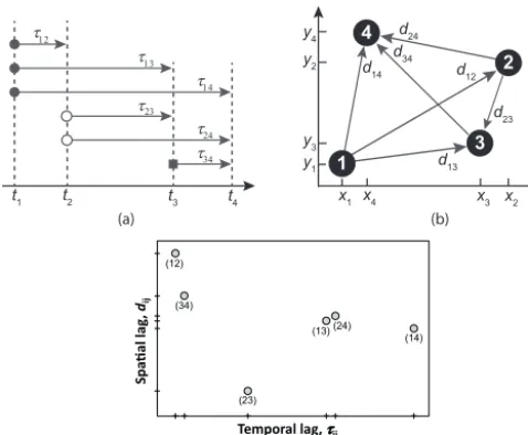
Figure 1.Illustration of our clustering analysis methodology.(a)A sequence of four point events occur at timest1,t2,t3,t4. The six temporal lagsτ12,τ13,τ14,τ23,τ24,τ34are shown.(b)The two-dimensional locations of the four point events are shown. The six spatial lags, d12, d13,d14,d23,d24,d34 are also shown.(c)The six spatial lags dij are shown as a function of the corresponding temporal lagsτij, whereiis the first event andjis the second event in time.
main shocks in both time and space. However, background seismicity (other main shocks) will also occur in the region and time interval in which the aftershocks occur. The back-ground seismicity will occur randomly in space and time, whereas the aftershocks of each background earthquake will be tightly clustered in space and time. It is important to sepa-rate the aftershocks from the background seismicity in order to study the statistics of the aftershocks. Zaliapin et al. (2008) demonstrated that plots of spatial lag vs. temporal lag clearly separated the two groups of earthquakes.
Here we consider the time and place of the touchdown of a tornado as a point event. Our studies will be concentrated on tornado outbreaks. An outbreak is a sequence of several to hundreds (Fuhrmann et al., 2014) of spatially correlated tornadoes that occur in a relatively short period of time, typi-cally a day, with generally fewer tornadoes at night as severe convection is inhibited. In contrast, earthquake aftershock se-quences are unrestricted in time by convective activity, and a severe earthquake of M=6 would typically generate thou-sands of aftershocks down toM=2 (e.g. Utsu, 1970) com-pared to a severe tornado outbreak involving just hundreds of tornadoes. Despite differences in process and scales between tornadoes and earthquakes, as discussed above, both tornado touchdowns and earthquake aftershocks can be considered as point events, and the spatial–temporal methodology devel-oped by Zaliapin et al. (2008) for seismicity is a very useful analysis for tornado outbreaks.
In this paper we will give several examples of tornado out-breaks, including maps of the tornado touchdown points as well as a clustering analysis of the dependence of spatial lag dij between the touchdowns of two tornadoes on the
tem-poral lagτij between the touchdown times of the same two
tornadoes. We consider each tornadoiand measure distance and times to each subsequent tornadojin the sequence. If the tornadoes occur randomly in space and time, the dependence of dij onτij will also be random. Alternatively, a tornado
outbreak could be a near-linear sequence of tornado touch-downs produced by a single supercell thunderstorm moving at a near-constant velocity. In this case, the dependence ofdij
onτij is approximately linear, and the slope is the velocity of
the convective cell.
To illustrate this clustering analysis methodology applied to tornadoes, we consider a sequence of four point events that occur at successive timest1,t2,t3,t4 and two-dimensional
locations (x1,y1), (x2,y2), (x3,y3), (x4,y4), as illustrated in
Fig. 1. The temporal lags (time differences) areτ12=t2−t1,
τ13=t3−t1,τ14=t4−t1,τ23=t3−t2,τ24=t4−t2andτ34=
t4−t3. The corresponding spatial lags (spatial separations)
ared12= [(x2−x1)2+(y2−y1)2]0.5andd13,d14,d23,d24
andd34determined in a similar way. The temporal lagsτ for
our four point events are illustrated in Fig. 1a and the spatial lagsd in Fig. 1b. The dependence of the spatial lagsd on the temporal lags τ are given in Fig. 1c. In this paper, we will show the dependence of spatial lags on temporal lags for pairs of tornado touchdowns.
The objective of this paper is to study the clustering statis-tics of tornado outbreaks. However, it must be recognized that the definition of a tornado outbreak is somewhat arbi-trary (Mercer et al., 2009). Ideally, the definition of a tor-nado outbreak would be the occurrence of multiple torna-does within a particular synoptic-scale weather system, but the spatial and temporal limits on the weather system are sub-ject to arbitrary distinction (Glickman, 2000). Galway (1977) classified tornado outbreaks into three types: (i) a local out-break with a radius less than 1000 miles (1609 km), (ii) a progressive outbreak moving from west to east in time and (iii) a line outbreak associated with a single moving super-cell thunderstorm. Unfortunately, the NOAA (2015) NWS– SPC database does not associate individual tornadoes with a specific tornado outbreak using any of these three (or other) classifications.
There is a strong diurnal variability in tornado occurrence associated with solar heating. For these reasons, Doswell et al. (2006) defined a tornado outbreak to include all torna-does in the continental USA in a convective day, i.e. the 24 h period from 12:00 UTC (Coordinated Universal Time) of a given day to 12:00 UTC of the following day, with 12:00 UTC (04:00 to 08:00 local time in the continental USA depending on month and location) corresponding to the ap-proximate time of the daily minimum in tornado occurrence. The Severe Weather Database that we use in our analyses list most tornadoes in Central Standard Time (CST), so we will consider tornadoes in a convective day as 06:00–06:00 CST. However, consistent with the studies of severe tornado out-breaks given by Malamud and Turcotte (2012), we will con-sider a severe tornado outbreak to include only those torna-does with path lengths L≥10 km. Elsner et al. (2015) de-veloped a method for separating distinct spatial clusters of tornado touchdowns during a convective day. Our methods differ in that we consider both space and time and are search-ing for near-linear features.
2 Clustering analysis of tornadoes
To illustrate our clustering analysis methodology for torna-does, we will first consider the intense tornado outbreaks in the central United States on 26 and 27 April 2011. The tor-nado outbreaks in the spring of 2011 have been discussed in detail by Doswell et al. (2012). They concluded that ideal conditions for severe tornado outbreaks occurred during the last 2 weeks of April 2011, and that the supercell thunder-storms responsible for the tornadoes were generated by a sequence of extratropical cyclones. In this paper, we focus our attention on the outbreaks that occurred on 26 and 27 April 2011. Although these outbreaks were certainly related to the same synoptic-scale weather pattern, we will treat the two outbreaks separately for our statistical studies. We will consider severe (L≥10 km) tornadoes on convective days: (i) 06:00 on 26 April to 06:00 CST on 27 April 2011 (i.e. a
0 50 100 150 200 250
To
rnado
pa
th
leng
th,
L
(km)
Time, t(h of day, CST)
06:00 12:00 18:00 00:00 06:00 12:00 18:00 00:00
06:00 12:00 18:00 00:00 00:00
26 April 2011 27 April 2011 28 April 2011
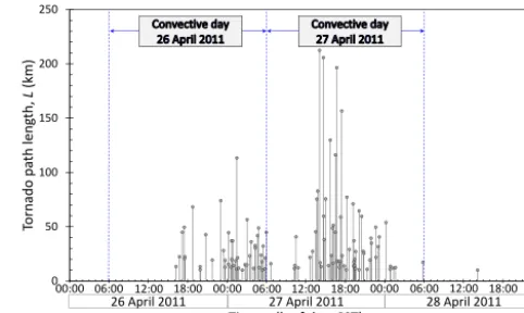
Figure 2.Tornado outbreak on 26–28 April 2011. Times of touch-down and path lengths of severe tornadoes (L≥10 km) that oc-curred on 26, 27 and 28 April 2011. There were 45 severe tornadoes on 26 April (convective day, 06:00 CST to 06:00 CST the following day) and 64 severe tornadoes on 27 April (convective day). Data were obtained from NOAA (2015).
convective day equivalent to 12:00 on 26 April to 12:00 UTC on 27 April 2011) and (ii) 06:00 on 27 April to 06:00 CST on 28 April 2011.
In Fig. 2 we give touchdown timest and path lengthsL for the 45 severe (L≥10 km) tornadoes that occurred on 26 April 2011 (convective day, 06:00 to 06:00 CST of the fol-lowing day) and for the 64 severe tornadoes that occurred on 27 April 2011 (convective day). In Malamud and Tur-cotte (2012), we suggested that a quantitative measure of the strength of a severe tornado outbreak is the total path length LD of all severe (L≥10 km) tornadoes in a convective day
in the continental USA. By this measure the strongest tor-nado outbreak during the 60-year period 1954–2013 was on 3 April 1974 (convective day) with 105 severe (L≥10 km) tornadoes and a total tornado path lengthLD=3852 km. For
the two outbreaks illustrated in Fig. 2, the outbreak on 26 April 2011 with 45 severe tornadoes had a total tornado path lengthLD=1239 km, the fifth strongest outbreak
dur-ing this same 60-year period, 1954–2013. The outbreak on 27 April 2011 with 64 severe tornadoes had a total path length LD=2815 km, the second strongest outbreak during this
pe-riod.
cut-31 32 33 34 35 36
96 95 94 93 92 91 90 89 88 87 86 85 84 83 82 81 80
To
uch
do
w
n
la
tit
ud
e (
○N)
Touchdown longitude (○W)
26 Apr 2011: 15:00–18:00 CST 26 Apr 2011: 18:00–21:00 CST 26 Apr 2011: 21:00–24:00 CST 27 Apr 2011: 00:00–03:00 CST 27 Apr 2011: 03:00–06:00 CST
A
B
(a) 26 April 2011 (tornado touchdown locations)
0 100 200 km
31 32 33 34 35 36 37 38 39 40 41 42 43 44
91 90 89 88 87 86 85 84 83 82 81 80 79 78 77 76 75
To
uch
do
w
n
la
tit
ud
e (
○N)
Touchdown longitude (○W) 27 Apr 2011: 06:00–09:00 CST
27 Apr 2011: 09:00–12:00 CST 27 Apr 2011: 12:00–15:00 CST 27 Apr 2011: 15:00–18:00 CST 27 Apr 2011: 18:00–21:00 CST 27 Apr 2011: 21:00–24:00 CST 28 Apr 2011: 00:00–03:00 CST 28 Apr 2011: 03:00–06:00 CST
(b) 27 April 2011 (tornado touchdown locations)
0 100 200 km
Figure 3.Tornado outbreak on 26–27 April 2011. Touchdown lo-cations of (a)45 severe (L≥ 10 km) tornadoes that occurred on 26 April 2011 (convective day, 06:00–06:00 CST) and(b) 64 se-vere (L≥10 km) tornadoes that occurred on 27 April 2011 (con-vective day). The touchdowns points for each tornado are given by colours and shapes (as given in the legend), representing successive 3 h intervals. The tornado path lengths for each tornado are given by thin black lines. In(a)the tornadoes outlined in the regions A and B will be discussed in a later section. Data were obtained from NOAA (2015).
off for a severe tornado) to 113.3 km (26 April 2011) and 212.4 km (27 April 2011). We will postpone a discussion of the regions A and B that are indicated on Fig. 3a until a later section. In Fig. 3a, although there tends to be a south-west to north-east trend to the 26 April 2011 touchdowns, the spa-tial distribution appears visually to be diffuse. In Fig. 3b, the south-west to north-east trend of the 27 April 2011 touch-downs is visually less diffuse than in Fig. 3a.
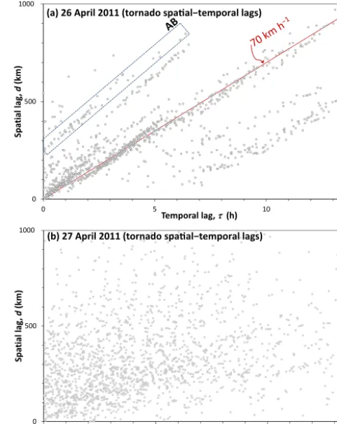
We now turn to our clustering analyses of the two tornado outbreaks on 26 and 27 April 2011. From the times of oc-currence given in Fig. 2 and the spatial locations of tornado touchdowns given in Fig. 3a and b, we obtain the tempo-ral and spatial lags using the method illustrated in Fig. 1. In Fig. 4a we give the spatial–temporal lag correlations of all pairs of the 45 severe (L≥10 km) tornado touchdowns that occurred on 26 April 2011 (convective day). The number of
0 500 1000
0 5 10
Spa
tial lag
,
d
(km)
Temporal lag, (h)
(b) 27 April 2011 (tornado spa al−temporal lags) 0
500 1000
0 5 10
Spa
tial lag
,
d
(km)
Temporal lag, (h)
(a) 26 April 2011 (tornado spa al−temporal lags)
Figure 4. Tornado outbreak on 26–27 April 2011. Spatial– temporal lag correlations between the touchdowns for(a)45 severe (L≥10 km) tornadoes that occurred on 26 April 2011 (convective day, 06:00–06:00 CST) and(b) 64 severe (L≥10 km) tornadoes that occurred on 27 April 2011 (convective day, 06:00–06:00 CST). The spatial lagdis plotted against the temporal lagτfor each of the (a)NP=990 pairs of tornado touchdowns and(b)NP=2016 pairs of tornado touchdowns. So that(a)and(b)have the same spatial– temporal limits, 147 (7 %) of the 2016 data points for(b)that have large spatial or temporal values are not included. The data points in Region AB in(a)are correlations between the spatial–temporal lags for the tornadoes in Region A and Region B in Fig. 3a.
pairs areNP=1+2+. . .+(NT−1), withNT the number
of tornadoes considered. WithNT=45 tornadoes, we have
NP=990 data points on the plot. There are quite clear
near-linear trends to thed (spatial lags) vs.τ (temporal lags) data given in Fig. 4a, with the spatial lags increasing with the tem-poral lags.
v=70 km h−1. A possible association is with the south-west to north-east movement of a single cell thunderstorm.
We next turn our attention to one of the near-linear trends in Fig. 4a that does not pass through the origin, indicated by the rectangular region AB. We return to Fig. 3a, where in Region A we outlined a spatial cluster of the touchdowns for three severe tornadoes that occurred on 26 April 2011 and, in Region B, a spatial cluster of the touchdowns for 14 se-vere tornadoes. In the rectangular region AB, given in Fig. 4a there are 51 data points of which 42 (82 %) represent all of the pairs of tornado touchdowns between the two regions A and B in Fig. 3a, with none of the data points in box AB as-sociated with pairs of tornadoes within Region A or pairs of tornadoes in Region B. We find that this explanation of corre-lations between tornadoes generated by two separate single cell thunderstorms (the spatial regions A and B in Fig. 3a) provides a similar explanation for the near-linear trends of spatial and temporal lags observed in Fig. 4a.
In Fig. 4b, we give the spatial lag vs. temporal lag for each of the pairs of the 64 severe (L≥10 km) tornado touchdowns that occurred on 27 April 2011 (convective day). In this case, there areNP=2016 pairs. Comparing Fig. 4b with Fig. 4a,
there are striking differences. Specifically, in Fig. 4b, there is no clear near-linear trend of the spatial–temporal lag data, whereas in Fig. 4a, this linear trend both through the origin and in other spatial–temporal lag regions of the plot is dom-inant. The near-random distribution of data points in Fig. 4b can be associated with the simultaneous generation of torna-does by several separately defined supercell thunderstorms. The resulting random generation of tornadoes both in space (the several supercells) and time (for each supercell) would lead to a near-random distribution of data points. The thun-derstorms on 26 April 2011 are much less likely to be super-cellular than those on 27 April 2011 (Knupp et al., 2013).
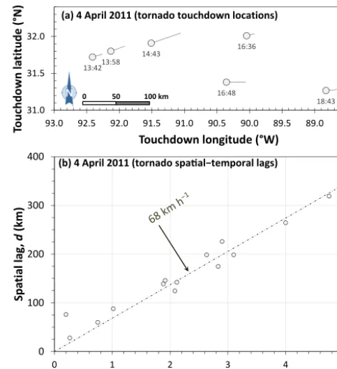
To further illustrate the relationship between tornadoes and storms, we apply our clustering analysis to severe torna-does that developed during a tornado outbreak that occurred in the south-east of the USA on 4 April 2011. During this out-break, an extensive squall line developed along and ahead of a cold front extending from Ohio in a south-westerly direc-tion to Mississippi and Louisiana (Corfidi et al., 2015). The environment proved suitable for the development of thun-derstorms within the largely linear convective band (Aon Benfield, 2011). The 4 April 2011 tornado outbreak is rec-ognized as a derecho event (Aon Benfield, 2011; NOAA, 2011; Corfidi et al., 2015), that is, a near-linear squall line dominated by straight-line high winds rather than cyclonic winds dominant in supercell thunderstorms. We consider six severe (L≥10 km) tornadoes that occurred between 13:42 and 18:43 CST. Three severe tornadoes on that day that were spatially distant (> 600 km from any of the six tornadoes) were not considered. The touchdown locations and tracks are given in Fig. 5a. In Fig. 5b, the spatial lag d is plotted against the temporal lagτ for each of these 15 pairs of tor-nado touchdown points, with a good linear correlation found.
13:4213:58
14:43 16:36
16:48
18:43 31.0
31.5 32.0
93.0 92.5 92.0 91.5 91.0 90.5 90.0 89.5 89.0 88.5
To
uchdown la
titude (°N)
Touchdown longitude (°W) 0 50 100 km
0 100 200 300 400
0 1 2 3 4 5
Spa
tial lag
,
d
(km)
Temporal lag, (h)
(a) 4 April 2011 (tornado touchdown locations)
(b) 4 April 2011 (tornado spa al−temporal lags)
Figure 5. Tornado outbreak on 4 April 2011. (a) Touchdown locations of six severe (L≥10 km) tornado that occurred on 4 April 2011 (convective day, 06:00 CST–06:00 CST) with touch-down times from 13:42 to 18:43 CST.(b)The spatial lagdis plotted against the temporal lagτfor each of the 15 pairs of tornado touch-down points. The straight-line fit to the data passing through the origin gives a velocityv=68.5 km h−1.
We compare the data values in Fig. 5b with a least-squares fit to a linear correlation passing through the origin, resulting in a supercell velocity ofv=68.5 km h−1 (Spearman rank correlation coefficient,r2=0.92).
One hypothesis for the 4 April 2011 tornado outbreak is that the tornadoes touched down randomly along the squall line. However, this hypothesis is not consistent with the data in Fig. 5b. Random spatial and random temporal touch-downs produce the random distribution of data points seen in Fig. 4b. The data in Fig. 5 require that the tornadoes are produced at a near-stationary point on the squall line as the squall line migrates at a near-uniform velocity.
A6 A9
B3
A12 E2
D1 E3
B17B18
D2 E6
D3 B20
G2
D4 H4
G5
D6
34.6 35.0 35.4 35.8 36.2
98.6 98.2 97.8 97.4 97.0 96.6 96.2 95.8
To
uchdown la
titude (°N)
Touchdown longitude (°W)
All storms (A,B,D,E,G,H) (18 tornadoes) Storm B (4 tornadoes)
Storm D (5 tornadoes) 0 50 100 km
0 100 200
0 1 2 3 4 5 6 7
Spa
tial lag
,
d
(km)
Temporal lag, (h)
All storms (A,B,D,E,G,H) (18 tornadoes) Storm B (4 tornadoes)
Storm D (5 tornadoes)
(a) 3 May 1999 (tornado touchdown locations)
(b) 3 May 1999 (tornado spa al−temporal lags)
Figure 6.Tornado outbreak on 3 May 1999 (convective day, 06:00– 06:00 CST).(a)Touchdown locations of 18 severe (L≥10 km) tor-nadoes, with storms A, B, D, E, G, H responsible for the tornadoes identified.(b)Spatial–temporal lag correlations between the touch-downs for (i) all 18 tornadoes given in(a), (ii) four tornadoes from Storm B, (iii) five tornadoes from Storm D. Also given are the best-fit lines for spatial–temporal lags for both Storms B and D. Data were obtained from NOAA (1999, 2015).
outbreak. The touchdown locations and tracks are given in Fig. 6a. Each of the tornadoes is associated with one of the six supercell thunderstorms designated A, B, D, E, G, H. The spatial and temporal lags have been obtained for all pairs of the 18 severe tornadoes using the method illustrated in Fig. 1. The results for the 153 spatial–temporal pairs are given in Fig. 6b. There are no clear linear patterns.
We will now focus our attention on the four severe torna-does associated with supercell B (shown in red in Fig. 6a) and the five tornadoes associated with supercell D (shown in blue in Fig. 6a). In Fig. 6b we designate spatial–temporal lags associated with supercell B (shown in red) and super-cell D (shown in blue). Clear linear patterns for the spatial– temporal lags associated with each of the two supercells are obtained. Also included are the best-fit lines for the spatial– temporal lags; for supercell B and D the velocities (slopes) are 43 and 38 km h−1respectively.
0 100 200 300 400 500
0 1 2 3 4 5 6
To
uch
down position,
x
(km)
Time of occurence, t(h)
80 km h‐1
(a)
0 100 200 300 400 500
0 1 2 3 4 5 6
Spa
tial lag
,
d
(km)
Temporal lag, (h)
80 km h‐1
(b)
Figure 7.Five model tornado touchdown points located randomly in time during a 6 h time window along a linear track.(a)The touch-down positionsx along the track are shown as a function of the random timest of occurrence. The model supercell thunderstorm responsible for the tornadoes moves along the track at a velocity
v=80 km h−1.(b)Spatial–temporal lag correlations between the 5 model tornadoes shown in Fig. 7a. The spatial lagd is plotted against the temporal lagτfor each of the 10 pairs of model tornado touchdown points. The data points again lie on a straight line with a slope of 80 km h−1.
through the origin are indicative of a progressive tornado out-break, possibly from a single supercell thunderstorm.
Confirmation of this behaviour has been obtained in our treatment of the 3 May 1999 outbreak. Severe tornadoes pre-viously associated with single supercell thunderstorms gen-erate spatial–temporal lag correlations that are well approx-imated by straight lines as illustrated in Fig. 6b. A similar linear correlation was shown for the six severe tornadoes we studied from the 4 April 2011 outbreak illustrated in Fig. 5b. We also suggest that the strong linear trends seen in the spatial–temporal correlation data for the 26 April 2011 out-break (Fig. 4a) may be associated with tornadoes generated by one or more single cell storms.
In order to further address the large difference in spatial–temporal correlations in the data illustrated in Fig. 4, we consider a second model, more complex than the one just given. In our second idealized model, we consider a quasi-linear vertical (north–south, y) “squall” line moving to the east at constant velocity v=80 km h−1 over an 800 km×800 km region and a 10 h period (for tornado touchdowns). Tornadic cells are distributed along the near-linear squall line with an approximate spacing 1y. Tornadoes are assumed to touch down at equally spaced time intervals (plus some noise εthat we introduce) 1t+ε. The ratio 1y/1t defines a characteristic velocity. Our hypothesis is that the non-dimensional velocity ratio B=(1y)/(v1t ) defines the behaviour of the system. If B is large (B> 1), quasi-linear behaviour is observed in the spatial–temporal lag domain. If B is small (B< 1), quasi-random behaviour is observed in the spatial–temporal lag domain. In Figs. 8 and 9, we give two model scenario examples. In Fig. 8a we consider four tornadic cells (each cell represented by a horizontal set of 10 circles, top to bottom) for which the vertical spacing between tornadic cells is1y≈(800 km)/4=200 km, and there are 10 tornado touchdowns from each cell so that 1t≈1 h with touch-down times indicated below each circle. The timing of the first tornado touchdown for each tornadic cell is chosen randomly within the first 1 h [(10 h)/(10 tornadoes)] plus some noiseεand spatially along the tornadic cell such that the first tornado touchdown occurs horizontally within the first 80 km (800 km 10 tornadoes−1). The non-dimensional parameter B=(1y)/(v1t )=(200 km)/[(800 km)/(10 tor-nadoes)=2.5. In Fig. 8b we consider 10 tornadic cells so that 1y≈(800 km)/10=80 km and four tornado touchdowns from each cell so that 1t≈2.5 h with the first tornado touchdown for each tornadic cell oc-curring randomly within the first 2.5 h [(10 h)/(4 tor-nadoes)] and horizontally within the first 200 km [(800 km)/(4 tornadoes)]. The non-dimensional param-eter B=(1y)/(v1t )=(80 km)/[(80 km h−1)(2.5 h)]=0.4. In Fig. 8 we give the tornado touchdown locations and times for both model scenarios 1 and 2, and in Fig. 9 the spatial– temporal lag results. For scenario 1 in Fig. 9a, withB=2.5, we obtain quasi-linear behaviour in the spatial–temporal lag
domain, which we consider further. The four tornadic lines from top to bottom in Fig. 8a are referred to as A (10 tor-nadoes alongy=725 km), B (y=475 km) C (y=300 km) and D (y=90 km). In Fig. 9a, the spatial–temporal lag do-main, the linear correlation passing through the origin results from lags within each of the four tornadic lines A, B, C and D. The next higher set of correlations in the spatial–temporal lag domain in Fig. 9a (starting at about d=200 km and τ=0 h) is a set of three lines adjacent to each other, which are the result of correlations between tornadic lines A and B, B and C and C and D. Similarly, the two sets of adjacent lines in Fig. 9a (starting at aboutd=400 km and τ =0 h) are the results of correlations between tornadic lines A and C and B and D. Finally, the single line in Fig. 9a (starting at aboutd=600 km andτ=0 h) is the result of correlation between the tornadic lines A and D in Fig. 8a. The model we consider is idealized, but we believe it illustrates conditions favourable for linear features (i.e. 26 April 2011) vs. more random features (i.e. 27 April 2011).
We now return to a discussion of the well-defined linear trends in the spatial–temporal correlation given in Fig. 4a. The first linear trend, extending from the origin with a slope corresponding tov=70 km h−1, can be explained as we ex-plained the similar linear trends in Figs. 5−7. For the second linear trend within the box AB of Fig. 4a, we determined that these points were the result of spatial–temporal correlations between the tornadoes in boxes A and B in Fig. 3a. Most of the data points (82 %) in box AB in Fig. 4a were the result of spatial–temporal lag correlations between boxes A and B in Fig. 3a. The approximately 300 km vertical offset distance at zero time lag in Fig. 4a between the origin and box AB is approximately the distance between the nearest touchdown locations between Region A and Region B in Fig. 3a. We at-tribute the curvature of secondary correlations in Fig. 9a to the initiation of the linear tracks in Fig. 8a at short time in-tervals. If the initiation of the tracks were offset for relatively large times, then straighter correlations would be expected.
We next introduce a measure of the combined spatial– temporal separation of pairs of tornado touchdowns, for which the spatial–temporal separationψis given by the fol-lowing:
ψ=τ+ d
vc
, (1)
12:23 13:27 14:19 15:20 16:18 17:28 18:28 19:25 20:23 21:23 12:30 13:32 14:32 15:32 16:32 17:24 18:34 19:34 20:24 21:31 12:04 13:05 14:07 15:03 16:07 17:04 18:06 19:03 20:02 21:05
12:51 13:53 14:53 15:56 16:57 17:50 18:48 19:51 20:52 21:53
0 200 400 600 800
0 200 400 600 800
y
(km)
x
(km)
(a) Scenario 1
12:50 15:23 17:47 20:19
12:53 15:21 17:52 20:28
12:31 14:57 17:25 20:05
13:06 15:36 18:00 20:35
13:10 15:45 18:04 20:42
13:17 15:42 18:14 20:49
12:48 15:22 17:53 20:18
14:17 16:41 19:15 21:47
12:07 14:43 17:07 19:33
13:05 15:34 18:00 20:34
0 200 400 600 800
0 200 400 600 800
y
(km)
x
(km)
(b) Scenario 2
Figure 8.Two model scenarios for 40 tornadoes in an 800 km×800 km region over a time period of 10 h.(a)Four parallel supercells moving at about 80 km h−1with 10 tornadoes each.(b)Ten parallel supercells moving at about 80 km h−1with four tornadoes each.
0 500 1000
0 5 10
Spa
tial
lag
,
d
(km)
Temporal lag, (h)
(a) Scenario 1
0 500 1000
0 5 10
Spa
tial
lag
,
d
(km)
Temporal lag, (h)
(b) Scenario 2
Figure 9.Spatial–temporal lag diagrams for the two model scenarios given in Fig. 8.
the normalized cumulative probability, defined as follows:
P (< ψ )=NC(< ψ )
NT
, (2)
withNC(<ψ ) the number of tornado touchdown pairs with
spatial–temporal separation values less than ψ andNT the
total number of pairs considered.
In Fig. 10 we plot the normalized cumulative probability P(<ψ )as a function of the spatial–temporal separationsψ. We consider the data for the two tornado outbreaks in the USA on 26 and 27 April 2011 (convective days) and utilize the values given in Fig. 3 for spatial–temporal separations ψ< 4 h. We have not considered data for the 4 April 2011 outbreak given in Fig. 5, because of the very small number of data points.
We see that the sets of normalized cumulative probabil-ity values for the two outbreaks given in Fig. 10 have a very different pattern, one linear and the other a power law. For the 26 April 2011, our data set consisted of 45 severe tor-nadoes resulting inNP=990 pairs of tornado touchdowns
of which 245 spatial–temporal separations are illustrated in Fig. 10. The least-squares best-fit linear correlation for the spatial–temporal separations for 26 April 2011, over the range 0.0 <ψ< 4.0 h, gives the following:
P (< ψ )=0.0671ψ−0.0241, (3) which is in excellent agreement with the data in the range 0.6 <ψ< 4.0 h. For the 27 April 2011 outbreak, our data set consisted of 64 severe tornadoes resulting inNP=2016 pairs
sep-26 April 2011(convective day):
P(<) = 0.0671− 0.0241, r² = 0.996
27 April 2011 (convective day):
P(<) = 0.0111.95, r² = 0.988
0.00 0.05 0.10 0.15 0.20 0.25
0 1 2 3 4
Normaliz
ed cumula
tiv
e pr
obability
, P(<
)
Spa al−temporal separa on(h)
Figure 10.Tornado outbreak on 26–27 April 2011. Normalized cu-mulative probabilityP(<ψ) of spatial–temporal separationsψ be-tween pairs of severe tornado (path lengthL≥10 km) touchdowns during tornado outbreaks in the USA on 26 and 27 April 2011 (con-vective days; see Figs. 2 and 3). Cumulative probabilities are given for spatial–temporal separations ψ < 4 h. The least-square best-fit line (blue dashed line) and power law (red dashed line) to the data are shown in this figure for 26 and 27 April 2011 respectively. Data were obtained from NOAA (2015).
arations are illustrated in Fig. 7. The least-squares best-fit power-law correlation for the spatial–temporal separations for 27 April 2011, over the range 0.0 <ψ< 4.0 h, gives the following:
P (< ψ )=0.011ψ1.95, (4)
which is in excellent agreement with the data and has an ex-ponent close to 2.
We now give an explanation for the linear and power-law correlations that we have found. If the tornado touch-downs occur randomly along a path for relatively small val-ues of spatial–temporal separations ψ, then a linear cor-relation of normalized cumulative probability P(<ψ ) with spatial–temporal separationψ is expected to be a good ap-proximation. In contrast, if the tornado touchdowns occur randomly in both space and time, then it is expected that P(<ψ )is proportional toψ2, i.e. the area of the segment of a circle of possible touchdown locations. The transition from linear to random behaviour indicated by the data in Fig. 10 is consistent with our previous qualitative discussion of the data given in Fig. 4.
3 Discussion
Unlike many other natural hazards, it is difficult to quantify strong tornadoes precisely. For hurricanes, there are exten-sive data on wind speeds and barometric pressures along the path of the storm. For floods, flood gauges provide a quan-titative measure of the flow rate in a river. For earthquakes,
seismographs give measures of shaking intensity. Quantify-ing volcanic eruptions and landslides is more difficult but volumes of material involved can be estimated. It is not pos-sible to reliably measure the wind speeds or pressure changes in tornadoes. The standard measure of tornado intensity used today is the Enhanced Fujita scale. This scale is based qual-itatively on the damage caused by a tornado. An alternative measure of tornado intensity is the tornado path lengthL.
Malamud and Turcotte (2012) showed that records of tor-nado path lengths from the 1990s to the present appear to be relatively complete for severe tornadoes (defined to beL≥10 km) in the United States. They also showed that the number-length scaling of severe tornado touchdowns is well approximated by a power-law distribution. Elsner et al. (2014) showed that the distribution of daily tornado counts in the United States is also well approximated by a power-law relationship. Malamud and Turcotte (2012) also studied the statistics of recent severe tornado outbreaks. They quantified the strength of a severe tornado outbreak to be the total tornado path lengthLD of the severe tornadoes
occur-ring duoccur-ring a convective day. They showed that the number-length scaling of severe tornado outbreaks is also well ap-proximated by a power-law distribution.
Another important aspect of tornado outbreaks is the dis-tribution of touchdown points in space and time. In terms of expectations for these data, there are two limiting cases.
i. Tornadoes occur randomly in space and time during a specified spatial region and time interval. In this case the touchdown points will be randomly distributed in space by interacting supercell thunderstorms.
ii. Tornadoes are generated by a single cell thunderstorm moving on a near-linear path at a constant velocity. In this case the touchdown points will approximately be on a linear path.
Actual tornado outbreaks will generally be a complex com-bination of these two limiting cases.
The statistics of the touchdown points of a tornado out-break can certainly be studied using a spatial map of the touchdown points. However, this does not directly incorpo-rate the time of the touchdowns. In this paper, we have con-sidered an alternative statistical measure for tornado touch-downs by applying a spatial–temporal clustering analysis originally developed by Zaliapin et al. (2008) for earth-quakes. The sequence of severe tornado touchdowns occur-ring duoccur-ring a convective day is considered to be a sequence of point events in space and time. All pairs of these point events are considered and a plot produced of the spatial lagd (i.e. spatial distance between the touchdown points for a pair of events) vs. the temporal lagτ(difference in touchdown times between the same pair of events).
convective day could be associated with tornadoes generated randomly along a linear squall line progressing at a near-constant velocity. In this case the tornado touchdowns oc-cur randomly both for space and time, and the cluster plot of d vs.τ would also be random. Alternatively, the tornadoes could be generated by a single cell thunderstorm moving in a near-linear path at a near-constant velocity. We have shown in Fig. 7 that in this case the points in ad vs.τ plot lie ap-proximately on a straight line through the origin, with the slope equal to the velocity of the thunderstorm. As a spe-cific example, we considered six severe tornado touchdowns associated with the 4 April 2011 derecho event in the south-eastern USA. The severe tornadoes could have been gener-ated randomly along the squall line. However, in Fig. 5b, we see that thedvs.τdata points lie approximately on a straight line through the origin with a slope of v=68 km h−1. This suggests that these six tornadoes were generated by a single large thunderstorm or several closely spaced thunderstorms moving at a velocity of about 68 km h−1.
To further illustrate the applicability of our clustering anal-ysis to severe tornado touchdowns, we considered the Great Plains tornado outbreak of 3 May 1999. Careful studies have associated individual tornadoes in the outbreak with spe-cific supercell thunderstorms as shown in Fig. 6b. When all 18 severe tornadoes are considered the data are quite ran-domly distributed. However, when two sets of tornadoes are considered that are associated with two supercell thunder-storms, clear linear patterns are obtained with slopes of 43 and 38 km h−1.
We also applied our clustering analysis to the intense tor-nado outbreaks in the central United States on 26 and 27 April 2011, with 45 and 64 severe tornadoes occurring re-spectively (convective days) and more than 300 fatalities. For each pair of tornadoes on the two separate days, the severe tornado touchdown spatial lags are given as a function of their temporal lags in Fig. 4. The observed patterns are very different. The results for 26 April 2011 (convective day) in Fig. 4a are dominated by a complex sequence of linear tracks that we have previously discussed. Knupp et al. (2013) sug-gest that this 26 April outbreak of tornadoes was associated with a quasi-linear convective squall line. The pattern seen in Fig. 4a has similarities to that seen in Fig. 5b but is clearly more complex. We suggest that on 26 April 2016 groups of these tornadoes were associated with one large thunderstorm or several closely spaced thunderstorms but there was a small number of groups that generated the complexity. This pattern is consistent with the movement of a discrete set of thunder-storms moving from the south-west to the north-east at veloc-ities near 70 km h−1. The observed pattern for 27 April 2011 (convective day) given in Fig. 4b is quite different. It is pre-dominantly random with virtually no embedded linear pat-terns. We suggest that this is due to a relatively large number of supercell thunderstorms generating tornadoes randomly in space and time.
In order to better understand the roles of supercell thun-derstorms in generating random and linear patterns in our spatial–temporal lag diagrams, we studied two model sce-narios for tornado generation. In the first model scenario (Fig. 8a), four supercell thunderstorms originating in a squall line each generated 10 tornadoes randomly. In the second model scenario (Fig. 8b), 10 supercell thunderstorms orig-inating in a squall line each generated four tornadoes ran-domly. The corresponding spatial–temporal lag diagrams for these two model scenarios are given in Fig. 9. The first scenario generated linear-type features; the second appeared random.
Although there are no physical processes directly in these two model scenarios, the statistical processes represent a va-riety of scales of processes that are important in tornado outbreaks. In general, the synoptic scale provides the back-ground that leads to convection over a broad area (e.g. Knupp et al., 2014). The spacing between storms and the timing of initiation depends upon relationships between the synoptic-scale and smaller-synoptic-scale features. Lilly (1979), Bluestein and Weisman (2000) and Lee et al. (2006) modelled the com-plexity of behaviour of storms that were initiated along lines; interaction included both constructive and destructive ones that can lead to the characteristic spacing associated with a particular event. Within a single supercell itself, the distance in time and space for repeated tornado genesis is a function of the storm motion (related to the large-scale environment in which the storm forms) and within-storm processes that lead to the distribution of precipitation and temperature lead-ing to the birth and death of rotation features in the storm (Burgess et al., 1982; Alderman et al., 1999). For a particu-lar tornado outbreak, the exact details depend upon the full range of atmospheric processes. Confidence is greatest in the understanding that certain large-scale environments are more likely to lead to outbreaks occurring, with details of individ-ual storm occurrence and withstorm features becoming in-creasingly less certain.
4 Data availability
NOAA (National Oceanic and Atmospheric Administration) Storm Prediction Centre (SPC), Tornado, Hail, and Wind Database, available at: www.spc.noaa.gov/wcm/.
Acknowledgements. The authors thank J. Elsner and one anony-mous referee for their helpful and constructive suggestions.
Edited by: R. Trigo
Reviewed by: J. Elsner, H. Brooks1, and one anonymous referee
References
Adlerman, E. J., Droegemeier, K. K., and Davies-Jones, R.: A numerical simulation of cyclic mesocyclogen-esis, J. Atmos. Sci., 56, 2045–2069, doi:10.1175/1520-0469(1999)056<2045:ANSOCM>2.0.CO;2, 1999.
Aon Benfield: United States April & May 2011 Severe Weather Outbreaks, Impact Forecasting, Aon Benfield (Chicago, USA) report, available at: http://www.aon.com/attachments/ reinsurance/201106_us_april_may_severe_weather_outbreaks_ recap.pdf (last access: 22 June 2016), 2011.
Bluestein, H. B. and Weisman, M. L.: The interaction of numerically simulated supercells initiated along lines, Mon. Weather Rev., 128, 3128–3149, doi:10.1175/1520-0493(2000)128<3128:TIONSS>2.0.CO;2, 2000.
Brooks, H. E.: On the relationship of tornado path length and width to intensity, Weather Forecast., 19, 310–319, doi:10.1175/1520-0434(2004)019<0310:OTROTP>2.0.CO;2, 2004.
Burgess, D. W., Wood, V. T., and Brown, R. A.: Mesocyclone evolu-tion statistics. 12th Conf. on Severe Local Storms, San Antonio, TX, Amer. Meteor. Soc., 422–424, 1982.
Corfidi, S. F., Coniglio, M. C., Cohen, A. E., and Mead, C. M.: A proposed revision to the definition of “derecho”, B. Am. Meteo-rol. Soc., 97, 935–949, doi:10.1175/BAMS-D-14-00254.1, 2015. Davies-Jones, R., Trapp, R. J., and Bluestein, H. B.: Tornadoes and tornadic storms, in: Severe Convective Storms, edited by: Doswell III, C. A., Meteorological Monographs, 167–221, Am. Meteorol. Soc., 2001.
Doswell III, C. A. and Burgess, D. W. Tornadoes and tornadic storms: A review of conceptual models, in: The Tornado: Its Structure, Dynamics, Prediction, and Hazards, edited by: Church, C., Burgess, D., Doswell III, C., and Davies-Jone, R., Geophys. Monogr., 79, 161–172, American Geophysical Union, Washington, D.C., 1993.
Doswell III, C. A., Edwards, R., Thompson, R. L., Hart, J. A., and Crosbie, K. C.: A simple and flexible method for rank-ing severe weather events. Weather Forecast., 21, 939–951, doi:10.1175/WAF959.1, 2006.
Doswell III, C. A., Brooks, H. E., and Dotzek, N.: On the imple-mentation of the enhanced Fujita scale in the USA, Atmos. Res., 93, 554–563, doi:10.1016/j.atmosres.2008.11.003, 2009.
1H. Brooks reviewed the discussion paper and was added as a
co-author during the revision.
Doswell III, C. A., Carbin, G. W., and Brooks, H. E.: The tornadoes of spring 2011 in the USA: An historical perspective, Weather, 67, 88–94, doi:10.1002/wea.1902, 2012.
Edwards, R., LaDue, J. G., Ferree, J. T., Scharfenberg, K., Maier, C., and Coulbourne, W. L.: Tornado intensity estimation: Past, present, and future, B. Am. Meteorol. Soc., 94, 641–653, doi:10.1175/BAMS-D-11-00006.1, 2013.
Elsner, J. B., Jagger, T. H., Widen, H. M., and Chavas, D. R.: Daily tornado frequency distributions in the United States, Environ. Res. Lett., 9, 024018, doi:10.1088/1748-9326/9/2/024018, 2014. Elsner, J. B., Elsner, S. C., and Jagger, T. H.: The increasing effi-ciency of tornado days in the United States, Clim. Dynam., 45, 651–659, doi:10.1007/s00382-014-2277-3, 2015.
Fuhrmann, C. M., Konrad, C. E., Kovach, M. M., McLeod, J. T., Schmitz, W. G., and Dixon, P. G.: Ranking of tornado outbreaks across the United States and their climatological characteris-tics, Weather Forecast., 29, 684–701, doi:10.1175/WAF-D-13-00128.1, 2014.
Galway, J. G.: Some climatological aspects of tornado out-breaks, Mon. Weather Rev., 105, 477–484, doi:10.1175/1520-0493(1977)105<0477:SCAOTO>2.0.CO;2, 1977.
Glickman, T. S. (Ed.): Glossary of Meteorology, 2nd Edn., Ameri-can Meteorological Society, 782 pp., 2000.
Knupp, K. R., Murphy, T. A., Coleman, T. A., Wade, R. A., Mullins, S. A., Schultz, C. J., Schultz, E. V., Carey, L., Sherrer, A., Mc-Caul Jr., E. W., Carcione, B., Latimer, S., Kula, A., Laws, K., Marsh, P. T., and Klockow, K.: Meteorological overview of the devastating 27 April 2011 tornado outbreak, B. Am. Meteorol. Soc., 95, 1041–1062, doi:10.1175/BAMS-D-11-00229.1, 2013. Lee, B. D., Jewett, B. F., and Wilhelmson, R. B.: The 19 April 1996
Illinois tornado outbreak. Part I: Cell evolution and supercell iso-lation, Weather Forecast., 21, 433–448, doi:10.1175/WAF944.1, 2006.
Lilly, D. K.: The dynamical structure and evolution of thunder-storms and squall lines, Annu. Rev. Earth Planet. Sc., 7, 117–161, 1979.
Malamud, B. D. and Turcotte, D. L.: Statistics of severe tornadoes and severe tornado outbreaks, Atmos. Chem. Phys., 12, 8459– 8473, doi:10.5194/acp-12-8459-2012, 2012.
Mercer, A. E., Shafer, C. M., Doswell III, C. A., Leslie, L. M., and Richman, M. B.: Objective classification of tornadic and nontor-nadic severe weather outbreaks, Mon. Weather Rev., 137, 4355– 4368, doi:10.1175/2009MWR2897.1, 2009.
NOAA (National Oceanic and Atmospheric Administration): Nor-mal Oklahoma National Weather Service Weather Forecast Of-fice, The Great Plains tornado outbreak of May 3–4, 1999, avail-able at: https://www.weather.gov/oun/events-19990503 (last ac-cess: 1 July 2016), 1999.
NOAA (National Oceanic and Atmospheric Administration): The Southeast US “Derecho” of April 4–5, available at: www.spc. noaa.gov/misc/AbtDerechos/casepages/apr042011page.htm (last access: 1 April 2016), 2011.
Utsu, T.: Aftershocks and earthquake statistics (1): Some parame-ters which characterize an afparame-tershock sequence and their interre-lations. J. of the Faculty of Science, Hokkaido University, Series 7 (Geophysics), 3, 129–195, 1970.