www.nat-hazards-earth-syst-sci.net/16/1897/2016/ doi:10.5194/nhess-16-1897-2016
© Author(s) 2016. CC Attribution 3.0 License.
Multi-objective optimization of typhoon inundation forecast models
with cross-site structures for a water-level gauging network by
integrating ARMAX with a genetic algorithm
Huei-Tau Ouyang
Department of Civil Engineering, National Ilan University, Yilan City, 26047, Taiwan
Correspondence to:Huei-Tau Ouyang ([email protected])
Received: 1 January 2016 – Published in Nat. Hazards Earth Syst. Sci. Discuss.: 23 February 2016 Revised: 12 July 2016 – Accepted: 19 July 2016 – Published: 16 August 2016
Abstract. The forecasting of inundation levels during ty-phoons requires that multiple objectives be taken into ac-count, including the forecasting capacity with regard to vari-ations in water level throughout the entire weather event, the accuracy that can be attained in forecasting peak water levels, and the time at which peak water levels are likely to occur. This paper proposed a means of forecasting inundation levels in real time using monitoring data from a water-level gauging network. ARMAX was used to construct water-level fore-cast models for each gauging station using input variables including cumulative rainfall and water-level data from other gauging stations in the network. Analysis of the correlation between cumulative rainfall and water-level data makes it possible to obtain the appropriate accumulation duration of rainfall and the time lags associated with each gauging sta-tion. Analyses on cross-site water levels as well as on cu-mulative rainfall enable the identification of associate sites pertaining to each gauging station that share high correla-tions with regard to water level and low mutual information with regard to cumulative rainfall. Water-level data from the identified associate sites are used as a second input variable for the water-level forecast model of the target site. Three in-dices were considered in the selection of an optimal model: the coefficient of efficiency (CE), error in the stage of peak water level (ESP), and relative time shift (RTS). A multi-objective genetic algorithm was employed to derive an op-timal Pareto set of models capable of performing well in the three objectives. A case study was conducted on the Xinnan area of Yilan County, Taiwan, in which optimal water-level forecast models were established for each of the four water-level gauging stations in the area. Test results demonstrate that the model best able to satisfy ESP exhibited significant
time shift, whereas the models best able to satisfy CE and RTS provide accurate forecasts of inundations when varia-tions in water level are less extreme.
1 Introduction
Typhoons are common weather events in subtropical regions of the Pacific, between July and October. Heavy rains carried in by typhoons often lead to the severe inundation of low-lying areas, which can damage property and even threaten the safety of human lives. Limitations in funding for construction of flood control systems pose limits to the protective capac-ity of structural measures for disaster mitigation. When the scale of a typhoon exceeds construction design limits, non-structural means are required to prevent disasters associated with typhoons. The real-time forecasting of changes in inun-dation depth in the hours after a typhoon is a crucial factor in the planning of relief operations.
siderable computing resources and can be very time con-suming, which makes it difficult to provide forecast infor-mation in real time for immediate disaster relief actions dur-ing typhoons. Black-box modeldur-ings are implemented in an entirely different manner. The process that occurs between rainfall and inundation is regarded as a black box, and no attempt is made to understand the underlying physical mech-anisms. Rather, the relationships between inputs and out-puts of the system are analyzed as a means of creating a black-box model. Although this approach is unable to ex-plain the physical phenomena, it provides an accurate repre-sentation of the relationship between inputs and outputs. Cal-culations can generally be completed more rapidly (Karlsson and Yakowitz, 1987), and information related to future varia-tions in water-level in inundated areas can be obtained in real time, which can be immensely helpful to decision making and disaster prevention.
A number of studies have applied black-box models to the problems of inundation or flooding. Karunanithi et al. (1994) proposed a cascade-correlation algorithm for the selection of neural network architectures and training algorithms and obtained encouraging results with regard to flow prediction. Thirumalaiah and Deo (1998) proposed the training of neu-ral networks using a selected sequence of previous flood observations at a specific location to enable real-time flood forecasting. Toth et al. (2000) compared the advantages and limitations of the auto-regressive moving average, artificial neural network (ANN), and non-parametric nearest-neighbor method in rainfall–runoff forecasting. They concluded that time series analysis is far more accurate than simple rain-fall predictions of a heuristic nature. Chang and Chen (2001) proposed a counter-propagation fuzzy-neural network capa-ble of automatically generating rules for use in clustering in-put data to enable streamflow prediction. Nayak et al. (2005) employed fuzzy computation in the development of a real-time flood forecasting model. They concluded that the recur-sive use of a one-step-ahead forecast model to predict flow using longer lead times produces results better than those achieved using independent fuzzy models for the forecast-ing of flow under various lead times. Chen et al. (2006) con-structed a flood forecast model using an adaptive neuro-fuzzy inference system (ANFIS). Their results demonstrated that ANFIS is superior to back-propagation neural network. Ro-manowicz et al. (2008) developed a data-based mechanis-tic methodology for the derivation of nonlinear dependence between water levels measured at gauging stations along a river. Kia et al. (2012) developed a flood model using vari-ous flood causative factors using ANN techniques and geo-graphic information system (GIS) for the modeling and sim-ulation of flood-prone areas in the southern parts of Peninsu-lar Malaysia. Pan et al. (2011) presented a real-time rainfall-inundation forecasting model using a hybrid neural network based on a synthetic database of inundation potential. Shiri et al. (2012) compared the performance of gene expression pro-gramming (GEP), ANFIS, and ANNs in the forecasting of
daily stream flow. They concluded that the GEP model out-performed the ANN and ANFIS models. Chen et al. (2012) utilized an ANN model and an ANFIS model to correct cal-culations in a two-dimensional hydrodynamic model used for the prediction of storm surge height during typhoon events. Najafzadeh and Zahii (2015) proposed the use of a neuro-fuzzy-based group method of data handling as an adaptive learning network for the prediction of flow discharge in straight compound channels.
In this study, we sought to develop a method for the fore-casting of inundation levels, based on data from a water-level gauging network during typhoons. We also performed a case study in which crucial model input variables were obtained by analyzing records from previous typhoons. Autoregres-sive moving average with exogenous inputs (ARMAX) was used to construct rainfall and water-level relationship mod-els of the gauging stations, and three indices were defined for the evaluation of model performance. A Pareto optimal model set was identified for the three indices using a multi-objective genetic algorithm (MOGA). Predicted water levels were compared with measured data to examine the perfor-mance of the optimal models subjected to each index.
This paper is organized as follows. The environmental background of the study area is introduced in Sect. 2. In Sect. 3, we explain ARMAX and the data analysis methods used to find suitable model input variables. We also intro-duce the indices used for the evaluation of the models. Sec-tion 4 presents the method used to identify the Pareto op-timal model set for the evaluation indices using a MOGA. Section 5 discusses the forecasting capability of the optimal models for each objective based on search results. Conclu-sions follow in Sect. 6.
2 Study area
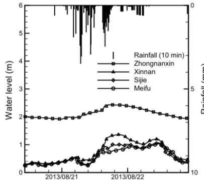
Yilan County (Fig. 1) is situated in the northeastern part of Taiwan. It has a subtropical monsoon climate and is famed for its rainy weather. With over 200 rain days per year, the annual average precipitation ranges between 2000 and 2500 mm. Yilan is bordered by mountains to the west and the ocean to the east. Typhoons are common in summer and autumn. Statistically, an average of two to three typhoons hit Taiwan each year, 45 % of which make landfall in Yilan County (Pan et al., 2014). Severe inundations quickly form in low-lying areas during typhoons. Among the inundation-prone regions, the area of Xinnan is one of the worst.
Table 1.Water-level gauging network in Xinnan area.
Gauging station Location Elevation above sea level (m) Longitude Latitude
Zhongnanxing 121.7877 24.7239 1.94
Xinnan 121.8012 24.7250 0.78
Sijie 121.8083 24.7234 0.13
Meifu 121.8156 24.7191 0.23
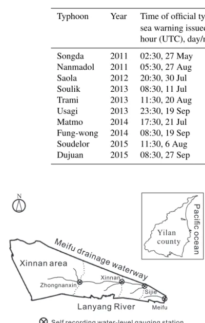
Table 2.Historical typhoon events recorded by SNTIX.
Typhoon Year Time of official typhoon Affecting Cumulative Maximum rainfall sea warning issued: period (h) rainfall (mm) intensity (mm h−1) hour (UTC), day/month
Songda 2011 02:30, 27 May 36 191.5 28.5
Nanmadol 2011 05:30, 27 Aug 99 159.5 26.5
Saola 2012 20:30, 30 Jul 90 506.0 35.5
Soulik 2013 08:30, 11 Jul 63 138.0 30.0
Trami 2013 11:30, 20 Aug 45 160.0 21.5
Usagi 2013 23:30, 19 Sep 63 158.0 24.0
Matmo 2014 17:30, 21 Jul 54 107.5 34.0
Fung-wong 2014 08:30, 19 Sep 72 79.5 37.5
Soudelor 2015 11:30, 6 Aug 69 462.5 86.0
Dujuan 2015 08:30, 27 Sep 57 226.0 41.5
Zhongnanxin
Xinnan
Sijie
Meifu Xinnan area
Meifu
drainage
waterway
Lanyang River
Yilan county
P
a
c
ifi
c
oc
e
a
n
N
Self recording water-level gauging station Drainage watercourse
Figure 1.Xinnan area in Yilan County, Taiwan.
out effectively, which soon leads to severe inundation. The safety and property of residents are in risk during typhoons, which underlines the need for effective disaster prevention measures.
In an attempt to better understand local inundation condi-tions during typhoons, the Water Resources Agency estab-lished the Surveillance Network for Typhoon Inundation in the Xinnan Area (SNTIX) in 2011. The network includes four gauging stations receiving water-level data on-site in the area and a data transmission system receiving precipita-tion observaprecipita-tion data from the QPESUMS (Quantitative Pre-cipitation Estimation and Segregation using Multiple Sensor;
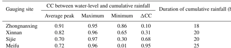
Gourley et al., 2002) of the Central Weather Bureau. Table 1 lists detailed information related to the gauging stations, the locations of which are marked in Fig. 1. SNTIX reports local inundation levels via radio transmission every 10 min dur-ing typhoons, while QPESUMS transmits 10 min rainfall in the area via internet connection at the same frequency. Fig-ure 2 presents the water levels recorded by SNTIX at gaug-ing stations and the QPESUMS rainfall data durgaug-ing Typhoon Trami in 2013. QPESUMS was developed jointly by the Cen-tral Weather Bureau and the National Severe Storm Labora-tory (NSSL) in 2002, with a view to improving the accu-racy of quantitative rainfall forecasts. QPESUMS comprises eight Doppler radar stations, each of which scans a radius of approximately 230 km. The system divides Taiwan into 441×56 grids, each covering 1.25×1.25 km2. Rainfall es-timation is achieved by obtaining readings from 406 rainfall gauges and 45 ground stations for adjustments. QPESUMS forecasts future rainfall patterns by predicting the movement paths of cloud cells. Data are provided for a wide range of applications, including typhoon rainfall forecasts (Lee et al., 2006), river flooding forecasts (Vieux et al., 2003), and land-slide forecasts (Chen et al., 2007).
Date
W
a
te
r
le
ve
l(
m
)
R
a
in
fa
ll
(mm)
2013/08/21 2013/08/22 0
1 2 3 4 5
6 0
5
10
Rainfall (10 min) Zhongnanxin Xinnan Sijie Meifu
Figure 2.Rainfall and water-level data recorded by SNTIX during typhoon Trami.
3 Model construction
To plan effective disaster prevention and relief operations during typhoons, it is crucial that one has the capacity to forecast inundation levels developing in the following hours. In the Xinnan area, inundation develops swiftly during ty-phoons, so forecasting must be quick and effective in or-der to provide sufficient lead time for decision making and operational planning. Thus, we adopted the ARMAX black-box model for the construction of water-level forecast mod-els for gauging stations. It should be noted that during ty-phoons, response plans rely more heavily on water levels than on runoff. We therefore based the forecast model on this study in the relationship between rainfall and water level rather than on the relationship between rainfall and runoff, as was common in many studies. Moreover, the rainfall and water-level data in this study were not processed in the con-ventional manner, in which the data are normalized by the maximum and minimum values before performing model re-gression, considering the fact that this information cannot be obtained while a typhoon is in progress. To enable real-time water-level forecasting during typhoons, we designed the level forecast model using raw rainfall and water-level data as inputs with the forecast water water-level of the next time step as the output.
3.1 ARMAX model
ARMAX (Box and Jenkins, 1976) is a linear black-box model that merges the AR model (Yule, 1927) and MA model (Slutzky, 1937) for time series analysis. It takes into account the influence of other external variables in the forecasting of
future changes in dynamic systems. The model is as follows:
A (q) y (t )= nu
X
i=1
Bi(q) ui(t−nki)+C (q) e(t ), (1)
wherey denotes the output of the system,ui stands for the
exogenous input for inputi,nuindicates the number of in-puts, nkiis the time lag for each input,eis the error term, and
A (q),Bi(q), andC (q)are the polynomial functions
com-posed of time shift operatorq.
In this study,y represents the water levels recorded at the gauging stations. To make full use of monitoring data from the surveillance network, each water-level model contains two exogenous inputs: rainfall datau1from QPESUMS and
water-level datau2 from an associate gauging station. The
structure of the model is determined by the number of terms in the four polynomial functionsA (q),B1(q),B2(q), and
C (q)and the time lags of the two exogenous inputs, nk1and
nk2. The coefficients of four polynomial functions can be
ob-tained by calibrating rainfall and water-level data. 3.2 Determination of input variables
In this study, we set the cumulative rainfall as the first input variable. After calculating the cumulative rainfall of various durations from 1 to 30 h, the results are subjected to corre-lation analysis using water-level data from the target site to derive the correlation coefficient (CC), which is defined as
CC(x,y)=cov(x, y) σxσy
=
Pn
i=1(xi−x)(yi−y) q
Pn
i=1(xi−x)2 q
Pn
i=1(yi−y)2 , (2)
where cov refers to the covariance between variablesxandy, σxandσyare the standard deviations ofxandy, respectively,
andndenotes the number of data points. CC ranges from−1 to 1, which indicate perfect negative correlation and perfect positive correlation betweenxandy, while a CC value of 0 indicates the complete absence of correlation.
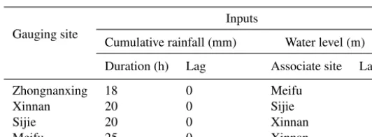
Table 3.Correlation coefficient (CC) between water-level and cumulative rainfall with average peak and the associated duration of cumulative rainfall.
Gauging site CC between water-level and cumulative rainfall Duration of cumulative rainfall (h)
Average peak Maximum Minimum 1CC
Zhongnanxing 0.91 0.95 0.86 0.10 18
Xinnan 0.82 0.96 0.65 0.31 20
Sijie 0.70 0.97 0.30 0.68 20
Meifu 0.72 0.96 0.01 0.95 25
rainfall corresponding to the peak average CC is longer in stations located further downward in the area. For instance, the duration of cumulative rainfall corresponding to the peak average CC at the Zhongnanxing station, which is at higher ground in the area, is 18 h, whereas the duration at the Meifu station, which is closest to the sea, is 25 h. We speculate that this might be associated with the time needed for water to ag-gregate and move downward. The table also presents a slight decrease in the peak average CC as the station falls closer to the sea as well as a greater difference between the maximum and minimum CC values. It is possible that this is because water levels at locations closer to the sea are influenced by ocean tides, which somewhat reduces its correlation with cu-mulative rainfall.
After identifying the duration of cumulative rainfall with the highest correlation for each gauging station, we analyzed the time lags between water levels and cumulative rainfall. We shifted back the cumulative rainfall data one time step at a time (each time step is 10 min) and calculated the CCs between water level and cumulative rainfall for each station. Figure 4a–d display the results of cross-correlation analysis for water levels and cumulative rainfall at each station. As can be seen, the peak average CC for each station occurred at zero lag, and the average CC decreases as the leg length-ened. This indicates that no time lag exists between water level and cumulative rainfall. Furthermore, the figures show that as the lag increased, not only the average but also the maximum and minimum CCs decreased, and the difference between the maximum and minimum CCs (1CC) gradually increased. This demonstrates that for all events the correla-tion between water level and cumulative rainfall during ty-phoons diminishes with the length of the lag.
To make full use of the water-level records from the gaug-ing stations, we identified an associate station for each exist-ing station and used the water levels from the associate sta-tion as a second input variable of the forecast models. Gen-erally speaking, the input and output of a model require a higher degree of correlation, while in between the input vari-ables a lower mutual information (MI) is expected (Bowden et al., 2005; Talei et al., 2010; Maier et al., 2010) in order to ensure that the information provided to the model from the
inputs are not redundant. MI is defined as MI(x,y)=1
2log(
|Cxx|
Cyy
|C| ), (3)
whereCis the covariance matrix defined as C=
Cxx Cxy
Cyx Cyy
, (4)
whereCxx andCyy are the variance of variables x andy,
respectively,Cxy andCyx are the covariance of variablesx
andy, and|C|is the absolute value of the determinant of the covariance matrix. An MI value equal to 0 indicates com-plete independence betweenxandy, while a higher MI value indicates stronger dependence betweenx andy (Fraser and Swinney, 1986; Moon et al., 1995).
To find an associate site with which the water-level data have a high CC with that of the target site while having a low MI with the identified cumulative rainfall of that specific site, we combined the two indices into
R=CC+(1−MI). (5)
The MI value presents the degree of dependence between the input variables; i.e., 1−MI reflects the degree of indepen-dence between input variables. The candidate site with the highest R value was designated as the associate site for a given target site. This approach in which MI is taken into ac-count in the selection of model inputs has been employed in previous studies (Talei et al., 2010; Elshorbagy et al., 2010; He et al., 2011).
Table 4.Selection of associate site for the second model input based onCCandMI.
Candidate site
Target site
CC between cross-site water levels MI between water-level input from candidate R(∗highest) site and cumulative rainfall input for target site
Zhongnanxing Xinnan Sijie Meifu Zhongnanxing Xinnan Sijie Meifu Zhongnanxing Xinnan Sijie Meifu
Zhongnanxing NA 0.81 0.76 0.70 NA 0.70 0.65 0.59 NA 1.12 1.11 1.11
Xinnan 0.81 NA 0.94 0.95 0.88 NA 0.72 0.66 0.94 NA 1.22∗ 1.29∗
Sijie 0.76 0.94 NA 0.95 0.88 0.87 NA 0.66 0.88 1.08 NA 1.29
Meifu 0.70 0.95 0.95 NA 0.68 0.81 0.73 NA 1.02∗ 1.14∗ 1.22 NA
Selected associate site Meifu Meifu Xinnan Xinnan
Table 5.Input variables for the water-level forecast models.
Gauging site
Inputs
Cumulative rainfall (mm) Water level (m)
Duration (h) Lag Associate site Lag
Zhongnanxing 18 0 Meifu
Xinnan 20 0 Sijie
Sijie 20 0 Xinnan
Meifu 25 0 Xinnan
to its slightly higherRvalue (to the third digit). The same sit-uation applies for Meifu station where both Xinnan and Sijie have practically identicalRvalues, and Xinnan was selected as the associate station for Meifu.
To elucidate the meaning of the time lag prior to variations in water-level data from target sites and their associate sites, we followed the previous analysis method in shifting water-level data from the associate sites one time step at a time. We then calculated the CCs between the water-level data from the target site and the associate site until we reached 30 time steps. The results in Fig. 5 show that the event-averaged CCs are all highest at zero lag. As the lag increases, the aver-age, maximum, and minimum CCs of each station decrease, and the difference between the maximum and minimum CCs gradually increases. This is a clear indication that no time lag exists between variations in water level measured at tar-get sites and at their associate sites. It is noted that, as shown in Fig. 5d, the mean CC for Meifu seems to be stationary for small time lags. The location of Meifu station is at the outlet of the area where it is close to the sea, as seen in Fig. 1. The water level at this site is likely to be influenced by factors other than rainfall and water level at the associate site (for example, tidal level of the sea). As a result, the cross-CC of Meifu to the associate site is the lowest compared to that of the other sites, as seen in Fig. 5d compared to Fig. 5a–c. This rather less connection of the cross-site water levels might re-sult in the somewhat stationary CC for small time lags. Still, as shown in Fig. 5d, while the mean CC seems to be station-ary for small time lags, the gradually expanding deviation between the maximum and minimum CCs of all the events
suggests a zero lag between the water levels at Meifu and its associate site.
The above data analysis makes it possible to determine the input variables of the water-level models for each station as well as their time lags, as shown in Table 5. The first input variable is cumulative rainfall, and the duration of cumulative rainfall in the various stations are not the same; however, all of the time lags are 0. The second input variable is water-level data from the associate site for which the time lags are also 0.
3.3 Model evaluation
The performance of each model was evaluated using the three indices below.
1. Nash–Sutcliffe coefficient of efficiency (CE) was pro-posed by Nash and Sutcliffe (1970) to assess the fore-casting capacity of hydrological models. It is defined as
CE=1− n
P
t=1
yobs(t )−yest(t )2
n
P
t=1
yobs(t )−yobs
2
, (6)
where yobs andyestdenote the observed and estimated
(a)
(b)
(c)
(d)
0 0.2 0.4 0.6 0.8 1
0 5 10 15 20 25 30
CC
Accumulation duration (h)
0 0.2 0.4 0.6 0.8 1
0 5 10 15 20 25 30
CC
Accumulation duration (h)
-0.2 0 0.2 0.4 0.6 0.8 1
0 5 10 15 20 25 30
CC
Accumulation duration (h)
-0.2 0 0.2 0.4 0.6 0.8 1
0 5 10 15 20 25 30
CC
Accumulation duration (h)
Figure 3.Correlations between water-level and cumulative rainfall over various durations:(a)Zhongnanxing station;(b)Xinnan sta-tion;(c)Sijie station;(d)Meifu station.
to 1 means that the water-level forecasts more closely match the observation data.
(a)
(b)
(c)
(d)
0 0.2 0.4 0.6 0.8 1
0 5 10 15 20 25 30
CC
Lag
0 0.2 0.4 0.6 0.8 1
0 5 10 15 20 25 30
CC
Lag
0 0.2 0.4 0.6 0.8 1
0 5 10 15 20 25 30
CC
Lag
0 0.2 0.4 0.6 0.8 1
0 5 10 15 20 25
CC
Lag
Figure 4.Cross-correlations between water level and cumulative rainfall with various time lags (10 min per lag):(a)Zhongnanxing station;(b)Xinnan station;(c)Sijie station;(d)Meifu station (cor-relation coefficient less than -0.2 is not shown).
2. Error in the stage of peak water-level (ESP) is calculated by
ESP=
yp,est−yp,obs
dp,obs
(a)
(b)
(c)
(d) 0
0.2 0.4 0.6 0.8 1
0 2 4 6 8 10 12 14 16 18 20 22 24 26 28 30
CC
Lag
0 0.2 0.4 0.6 0.8 1
0 2 4 6 8 10 12 14 16 18 20 22 24 26 28 30
CC
Lag
0 0.2 0.4 0.6 0.8 1
0 2 4 6 8 10 12 14 16 18 20 22 24 26 28 30
CC
Lag
0 0.2 0.4 0.6 0.8 1
0 2 4 6 8 10 12 14 16 18 20 22 24 26 28 30
CC
Lag
Figure 5.Cross-correlations of between-site water levels with var-ious time lags (10 min per lag):(a)Zhongnanxing station;(b) Xin-nan station;(c)Sijie station;(d)Meifu station.
whereyp,obsandyp,estdenote the peak observed and
es-timated water levels, respectively, anddp,obsis the peak
observed water depth. ESP represents the error between the peak observed water level and the forecast results of the model. A smaller ESP value means that the es-timated peak water levels more closely match the ob-served values.
3. Relative time shift (RTS): previous researches have shown that using historical data to forecast future changes often results in time shift errors between the forecast and measured hydrographs (Dawson and Wilby, 1999; Jain et al., 2004; de Vos and Rientjes, 2005). To evaluate the time shift error of forecast water levels, we shifted the forecast water-level hydrograph back by 1 to 18 time steps and then calculated the CE values. The time step corresponding to the highest CE value is the time shift error (δ) of the water-level model. This method was also adopted by de Vos and Rientjes (2005) and Talei et al. (2010). The RTS of the models in this study was defined as
RTS= δ
Lt
, (8)
whereδdenotes the time shift error of the model, andLt
is the prediction lead time of the model. A smaller RTS refers to a smaller time shift error between the forecast and observed water levels.
The determination of the prediction lead time depends on the required action time for relief operations during typhoons, such as evacuating people from the flooded area. In practice, it would be better to have at least 3 h ahead to warrant a smooth operation. Thus,Lt is set to
be 3 h for discussion in the present study. However, it should be noted that the proposed methodology is ap-plicable to any prediction lead time.
3.4 Cross validation
Cross validation (Geisser, 1993) was adopted for model cali-bration and typhoon event validation. For each model with a designated model structure (i.e., the number of terms for each of the four polynomialsA (q),B1(q),B2(q), andC (q)), a
single typhoon event was first selected for model validation and all the other nine events were used to calibrate the set of the model parameters (i.e., the coefficients of the four poly-nomials). The procedure was repeated by selecting another event for validation and all the other events for calibration. Each time the CE, ESP, and RTS scores from the validation case were computed and recorded. In turn, all of the typhoon events were validated, and the performance of this model structure was then represented by the averaged CE, ESP, and RTS over all the validation cases. This procedure was inte-grated with a MOGA introduced in the following to search for the optimal models that perform well in all the three in-dices for each gauging station.
4 Multi-objective optimization
wa-ter levels), and RTS (to dewa-termine the time at which a peak water level occurs), each provide crucial element to disas-ter prevention operations during typhoons and must therefore be considered simultaneously. Unfortunately, it is difficult to weigh the importance of each element. Thus, we employed multi-objective optimization to search for models capable of performing well in all three indices.
4.1 Objective functions and Design variables
The design goals included a larger CE and smaller ESP and RTS. Thus, we defined the objective function as follows:
Objective 1: minimize(1−CE), (9)
Objective 2: minimizeESP, (10)
Objective 3: minimizeRTS, (11)
where CE, ESP, and RTS denote the typhoon-event averages of the three indices.
As mentioned previously, the structure of the ARMAX model is determined by the polynomial functions A (q), B1(q),B2(q), andC (q)and the time lags of the two
exoge-nous inputs, nk1and nk2. The time lags can be derived from
previous data analysis. The analysis of time lag between cu-mulative rainfall and water levels at the associate site shows that the time lags between the two inputs and the output of the model are both 0. QPESUMS is able to provide forecasts on rainfall in the following time step; therefore, we set nk1to
0 in order to incorporate the rainfall predictions provided by QPESUMS within the models. Because we have only real-time monitoring values (rather than forecast values) for the water level at associate sites, we set nk2to 1. Thus, the
struc-ture of the model is determined by the remaining number of terms in the polynomial functions. Thus, we set the de-sign variables as the number of terms in the four polynomial functions, which are integers and limited the range of each design variable to between 1 and 10 in order to preserve the simplicity of the model.
4.2 Multi-objective genetic algorithm
A lack of continuous relationships between the structure of the model and the objective function makes it impossible to obtain the optimal value of this problem using a gradient-based method. Based on the characteristics of the problem, we employed a genetic algorithm (GA) as a tool for opti-mization due to the fact that GAs do not require the Hessian matrix of the objective function to derive the optimal solution for each design variable. Furthermore, the fact that GAs can search for global optimums (Goldberg, 1989) makes this an extremely suitable approach to the identification of an ideal model.
GAs are based on Darwin’s theory of natural selection. Since Holland (1973) developed a sound mathematical foun-dation based on this principle, GAs have been widely ap-plied in a variety of fields to solve problems that could not
otherwise be solved using conventional methods. In GAs, the individuals in a group are viewed as possible solutions to the problem under discussion. The individuals are rated according to their performance as they pertain to the ob-jective functions and constraints. Superior performance in-creases the chance of passing on genes to the next gener-ation. Through this process, the overall performance of the population gradually evolves and improves. After evolving for several generations, individuals with optimal genes (i.e., those that dominate the population) are adopted as the opti-mal solutions to the problem. GAs conduct optimization by assessing the performance of individuals in the population, which makes them ideally suited to solving problems with multiple objectives.
In MOGA, the first generation of models for each gaug-ing sites were produced by randomly specifygaug-ing the number of terms of the four polynomials andC (q), for each of the models. The performance of each model was evaluated by the three indices, obtained by the cross validation procedure introduced in Sect. 3.4. MOGA then produced the next gen-eration of models based on the performance of each individ-ual model. The procedure iterated until a stopping criterion was reached. Through this process, the whole generation of models gradually evolved, and a Pareto model set containing models that perform well in all three indices was gradually generated. In the present study, the population size in MOGA was set at 50 for each gauging site and the Pareto fraction at 0.35. The maximum number of evolutionary generations was 200, and the MOGA was set to terminate after the results stalled for more than 20 generations.
5 Results and discussion
The result of the MOGA is a Pareto optimal set. All of the models in this set are un-dominated, which means that at least one of their three indices (CE, ESP, and RTS) is not sur-passed by that of any other model. We selected the models with the best performance in all three indices from the Pareto optimal set, the results of which are as shown in Table 6. We listed three models for each gauging station and named them according to their location. For example, the models for Zhongnanxing station are Z1, Z2, and Z3. Among the three model types, model type 1 achieved the highest average CE, model type 2 achieved the lowest average ESP, and model type 3 achieved the lowest average RTS. The table lists four integer design variables for each model, indicating the num-ber of terms inA (q),B1(q),B2(q), andC (q). The table
also displays the scores of each model type on the three in-dices, wherein the score marked with an asterisk achieved the optimal value for that index.
Table 6.Models selected from the Pareto optimal model set using the best scores for each of the three objectives (∗best score).
Gauging site Model Objective Design variables CE ESP RTS
Zhongnanxing
Z1 max CE [9 9 4 8] 0.82∗ 0.14 0.42
Z2 min ESP [1 4 1 1] 0.73 0.03∗ 0.84
Z3 min RTS [10 10 8 6] 0.69 0.19 0.36∗
Xinnan
X1 max CE [10 4 6 3] 0.82∗ 0.06 0.38
X2 min ESP [1 2 2 3] 0.67 0.03∗ 0.99
X3 min RTS [5 5 4 3] 0.72 0.20 0.17∗
Sijie
S1 max CE [8 3 2 1] 0.66∗ 0.12 0.68
S2 min ESP [1 1 1 2] 0.50 0.04∗ 0.99
S3 min RTS [3 6 7 6] 0.10 0.26 0.33∗
Meifu
M1 max CE [8 8 6 8] 0.65∗ 0.21 0.57
M2 min ESP [1 1 5 3] 0.55 0.02∗ 0.97
M3 min RTS [9 5 7 5] 0.33 0.22 0.23∗
Date/time
W
a
te
r
le
v
e
l
(m
)
2012-08-02 2012-08-03 2
2.4 2.8 3.2
Data Z1 Z2 Z3
Date/time
W
a
te
r
le
v
e
l
(m
)
2012-08-02 2012-08-03 0.8
1.2 1.6 2.0
2.4 Data
S1 S2 S3
Date/time
W
a
te
r
le
v
e
l
(m
)
2012-08-02 2012-08-03 0.8
1.2 1.6 2.0 2.4 2.8
Data X1 X2 X3
Date/time
W
a
te
r
le
v
e
l
(m
)
2012-08-02 2012-08-03 0.8
1.2 1.6 2.0
2.4 Data
M1 M2 M3
(b) (d)
(a) (c)
Figure 6.Comparison of model predictions (3 h lead time) and measured data at(a)Zhongnanxing station;(b)Xinnan station;(c)Sijie station;(d)Meifu station.
show that the forecast water levels from the three models of the Zhongnanxing station (furthest from the sea) are roughly identical to the observed water levels, indicating that the fore-cast results are very accurate. No significant differences were observed among the forecast results of the three model types. The forecast results of the other three gauging stations in Fig. 6b, c, and d by the three types of models present different characteristics. Model type 2 (X2, S2, and M2) shows good performance in predicting peak water levels while exhibiting
particu-(a)
(b)
(c) 0
0.2 0.4 0.6 0.8 1
Z1 Z2 Z3 X1 X2 X3 S1 S2 S3 M1 M2 M3
CE
Model
0 0.2 0.4 0.6 0.8 1
Z1 Z2 Z3 X1 X2 X3 S1 S2 S3 M1 M2 M3
ESP
Model
0 0.2 0.4 0.6 0.8 1
Z1 Z2 Z3 X1 X2 X3 S1 S2 S3 M1 M2 M3
RTS
Model
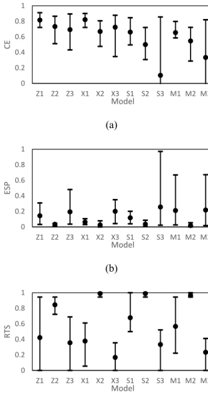
Figure 7.Comparison of model performance:(a)CE;(b)ESP;(c)
RTS.
larly apparent at the Sijie station in Fig. 6c and at the Meifu station in Fig. 6d, where water levels rose swiftly. However, the time shift errors presented by model types 1 and 3 are still smaller than 3 h. Considering that the lead time used in these model forecasts was 3 h, any time shift error of less than 3 h means that the results retain reference value for disaster pre-vention operations during typhoons. It is worth noting that, as shown in Fig. 6, the predicted hydrographs exhibit cer-tain fluctuation compared to the data. The reason for this is that the input of the models includes rainfall data recorded with a frequency of 10 min. As seen in Fig. 2, the rainfall data record appears to be fluctuating through the event. As a result, the hydrographs predicted by the models also dis-play certain fluctuations. However, the trend of the predic-tions still matches the observapredic-tions.
Figure 7a–c present the variation of CE, ESP, and RTS, respectively, among the models. As shown in Fig. 7a,
com-pared to the type 2 and type 3 models, model type 1 (Z1, X1, S1, and M1) exhibit higher mean CEs as well as smaller deviations between the max and the min. Among the four type 1 models, models Z1 and X1 achieve higher mean CE than models S1 and M1. The reason for this might be that the locations of Sijie station and Meifu station are more closer to the sea and the water levels at these sites might be influ-enced by other factors (such as tidal levels) not accounted for in the models. Figure 7b shows the variation of ESP among the models. It is clearly seen that type 2 models (Z2, X2, S2, and M2) display mean ESP values much lower than the other two types of models. The deviations of ESP for type 2 models are also much smaller compared to those of the other types of models. This demonstrates the good performance of type 2 models on peak water-level prediction. As seen in Fig. 7b, type 3 models (Z3, X3, S3, and M3) appear to dis-play poorer performance on peak water-level prediction, in-dicated by higher mean ESP as well as larger deviations. It is noted that, while type 2 models exhibit very low ESP on peak water prediction, they also suffer from severe time shift errors, as signified by the rather high RTS of these models shown in Fig. 7c. In contrast, type 3 models (Z3, X3, S3, and M3) exhibit much lower mean RTS than the type 2 models. In comparing the RTS performance of type 1 and type 3 models, it appears that model Z3 performs slightly better than Z1 at Zhongnanxing station, while at the other stations, the type 3 models achieve rather better RTS scores than type 1 models. In summary, type 1 models achieve the best score on CE with moderate performance on ESP and RTS. Type 2 and type 3 models display somewhat opposite characteristics. Type 2 models exhibit good performance on predicting the peak water level but also show rather severe time shift errors. In contrast, type 3 models achieve good scores on RTS but perform poorly on ESP.
6 Conclusions
the Pareto model set. Comparisons with measured water lev-els show that the modlev-els emphasizing ESP (model type 2) resulted in accurate prediction on the peak water levels but also show noticeable time lag. The models emphasizing CE (model type 1) and RTS (model type 3) provided an accu-rate indication of variations in water levels with no lag while water levels were dropping, yet a slight time lag when wa-ter levels were rising. Comparisons on the variations of per-formance indices among the models indicate that, in general, type 1 models present the best performance on CE with mod-est ESP and RTS. Type 2 models achieve very good perfor-mance on ESP but suffer from time shift errors. In contrast, type 3 models display good performance on RTS, though they are somewhat poorer on ESP. The results show that the proposed methodology is capable of deriving optimal mod-els each showing good performance on the three indices. All three types of models together provide thorough information in a real-time manner and are expected to be of help for dis-aster prevention operations during typhoons.
7 Data availability
The data set is available at: http://fhy.wra.gov.tw/fhy/Alert/ Water.
Acknowledgements. This research was supported by the Ministry of Science and Technology in Taiwan under grant no. MOST 105-2625-M-197-001. Support from the Water Resources Agency in Taiwan is also gratefully acknowledged.
Edited by: S. Tinti
Reviewed by: two anonymous referees
References
Bowden, G. J., Dandy, G. C., and Maier, H. R.: Input determination for neural network models in water resources applications. Part 1 – background and methodology, J. Hydrol., 301, 75–92, 2005. Box, G. E. and Jenkins, G. M.: Time series analysis: forecasting and
control, revised ed., Holden-Day, 569–570, 1976.
Chang, F. J. and Chen, Y. C.: A counterpropagation fuzzy-neural network modeling approach to real time streamflow prediction, J. Hydrol., 245, 153–164, 2001.
Chen, C. Y., Lin, L. Y., Yu, F. C., Lee, C. S., Tseng, C. C., Wang, A. H., and Cheung, K. W: Improving debris flow monitoring in Tai-wan by using high-resolution rainfall products from QPESUMS, Nat. Hazards, 40, 447–461, 2007.
Chen, S. H., Lin, Y. H., Chang, L. C., and Chang, F. J.: The strat-egy of building a flood forecast model by neuro-fuzzy network, Hydrol. Process., 20, 1525–1540, 2006.
Chen, W.-B., Liu, W.-C., and Hsu, M.-H.: Predicting typhoon-induced storm surge tide with a two-dimensional hydrody-namic model and artificial neural network model, Nat. Hazards Earth Syst. Sci., 12, 3799–3809, doi:10.5194/nhess-12-3799-2012, 2012.
Dawson, C. W. and Wilby, R.: An artificial neural network approach to rainfall-runoff modelling, Hydrol. Sci. J., 43, 47–66, 1998. de Vos, N. J. and Rientjes, T. H. M.: Constraints of artificial neural
networks for rainfall-runoff modelling: trade-offs in hydrological state representation and model evaluation, Hydrol. Earth Syst. Sci., 9, 111–126, doi:10.5194/hess-9-111-2005, 2005.
Elshorbagy, A., Corzo, G., Srinivasulu, S., and Solomatine, D. P.: Experimental investigation of the predictive capabilities of data driven modeling techniques in hydrology – Part 1: Con-cepts and methodology, Hydrol. Earth Syst. Sci., 14, 1931–1941, doi:10.5194/hess-14-1931-2010, 2010.
Fraser, A. M. and Swinney, H. L.: Independent coordinates for strange attractors from mutual information, Phys. Rev.-A, 33, 1134, doi:10.1103/PhysRevA.33.1134, 1986.
Geisser, S.: Predictive Inference, New York, NY, Chapman and Hall, 32–33, 1993.
Goldberg, D. E.: Genetic Algorithms in Search, Optimization, and Machine Learning, Addison Wesley, 7–10, 1989.
Gourley, J. J., Maddox, R. A., Howard, K. W., and Burgess, D. W.: An exploratory multisensor technique for quantitative estimation of stratiform rainfall, J. Hydrometeorol., 3, 166–180, 2002. He, J., Valeo, C., Chu, A., and Neumann, N. F.: Prediction of
event-based stormwater runoff quantity and quality by ANNs devel-oped using PMI-based input selection, J. Hydrol., 400, 10–23, 2011.
Holland, J. H.: Genetic algorithms and the optimal allocation of tri-als, SIAM J. Comp., 2, 88–105, 1973.
Jain, A., Sudheer, K. P., and Srinivasulu, S.: Identification of phys-ical processes inherent in artificial neural network rainfall runoff models, Hydrol. Process., 18, 571–581, 2004.
Karlsson, M. and Yakowitz, S.: Rainfall-runoff forecasting meth-ods, old and new. Stoch. Hydrol. Hydraul., 1, 303–318, 1987. Karunanithi, N., Grenney, W. J., Whitley, D., and Bovee, K.: Neural
networks for river flow prediction, J. Comput. Civil Eng., 8, 201– 220, 1994.
Kia, M. B., Pirasteh, S., Pradhan, B., Mahmud, A. R., Sulaiman, W. N. A., and Moradi, A.: An artificial neural network model for flood simulation using GIS: Johor River Basin, Malaysia, Envi-ron. Earth Sci., 67, 251–264, 2012.
Lee, C. S., Huang, L. R., Shen, H. S., and Wang, S. T.: A climatol-ogy model for forecasting typhoon rainfall in Taiwan, Nat. Haz-ards, 37, 87–105, 2006.
Maier, H. R., Jain, A., Dandy, G. C., and Sudheer, K. P.: Methods used for the development of neural networks for the prediction of water resource variables in river systems: current status and future directions, Environ. Model. Softw., 25, 891–909, 2010. Moon, Y. I., Rajagopalan, B., and Lall, U.: Estimation of mutual
information using kernel density estimators, Phys. Rev. E, 52, 2318–2321, 1995.
Najafzadeh, M. and Zahiri, A.: Neuro-Fuzzy GMDH-Based Evolutionary Algorithms to Predict Flow Discharge in Straight Compound Channels, J. Hydrol. Eng., 20, 04015035, doi:10.1061/(ASCE)HE.1943-5584.0001185, 2015.
Nash, J. and Sutcliffe, J. V.: River flow forecasting through concep-tual models part I – A discussion of principles, J. Hydrol., 10, 282–290, 1970.
Pan, T.-Y., Lai, J.-S., Chang, T.-J., Chang, H.-K., Chang, K.-C., and Tan, Y.-C.: Hybrid neural networks in rainfall-inundation forecasting based on a synthetic potential inundation database, Nat. Hazards Earth Syst. Sci., 11, 771–787, doi:10.5194/nhess-11-771-2011, 2011.
Pan, T. Y., Chang, L. Y., Lai, J. S., Chang, H. K., Lee, C. S., and Tan, Y. C.: Coupling typhoon rainfall forecasting with overland-flow modeling for early warning of inundation, Nat. Hazards, 70, 1763–1793, 2014.
Romanowicz, R. J., Young, P. C., Beven, K. J., and Pappenberger, F.: A data based mechanistic approach to nonlinear flood routing and adaptive flood level forecasting, Adv. Water Resour., 31, 1048– 1056, 2008.
Shiri, J., Ki¸si, Ö., Makarynskyy, O., Shiri, A. A., and Nikoofar, B.: Forecasting daily stream flows using artificial intelligence ap-proaches, J. Hydraul. Eng., 18, 204–214, 2012.
Slutzky, E.: The summation of random causes as the source of cyclic processes, Econometrica, 105–146, 1937.
Talei, A., Chua, L. H. C., and Wong, T. S.: Evaluation of rainfall and discharge inputs used by Adaptive Network-based Fuzzy Infer-ence Systems (ANFIS) in rainfall–runoff modeling, J. Hydrol., 391, 248–262, 2010.
Thirumalaiah, K. and Deo, M. C.: Real-time flood forecasting using neural networks, Comp. Aid. Civil. Infrastruct. Eng., 13, 101– 111, 1998.
Toth, E., Brath, A., and Montanari, A.: Comparison of short-term rainfall prediction models for real-time flood forecasting, J. Hy-drol., 239, 132–147, 2000.
Vieux, B. E., Vieux, J. E., Chiarong, C., and Howard, K. W.: Oper-ational deployment of a physics-based distributed rainfall-runoff model for flood forecasting in Taiwan, IAHS-AISH publication, 251–257, 2003.