Analysis and Modeling of Mobile Traffic Using Real Traces

Analysis and Modeling of Mobile Traffic

Using Real Traces

Hoang Duy Trinh

_{, Nicola Bui}

_{, Joerg Widmer}

_{, Lorenza Giupponi}

_{, Paolo Dini}

†_{CCIS, Northeastern University, Boston, MA, United States} ‡_{IMDEA Networks Institute, Leganes, Madrid, Spain}

Abstract—The analysis of real mobile traffic traces is

helpful to understand usage patterns of cellular networks. In particular, mobile data may be used for network op-timization and management in terms of radio resources, network planning, energy saving, for instance. However, real network data from the operators is often difficult to be accessed, due to legal and privacy issues. In this paper, we overcome the lack of network information using a LTE sniffer capable of decoding the unencrypted LTE control channel and we present a temporal and spatial analysis of the recorded traces. Moreover, we present a methodology to derive a stochastic characterization for the daily variation of the LTE traffic. The proposed model is based on a discrete-time Markov chain and is compared with the real traces. Results show that, with a limited number of states, our model presents a high level of accuracy in terms of first and second order statistics.

I. INTRODUCTION

Understanding the utilization of the actual network resources is fundamental for building solid models that can be used to design efficient mobile networks. With the advent of new 5G paradigms and the tremendous increase of the Internet usage, there is the need for finding efficient radio resource management and net-work planning solutions that will exploit and extend the actual resources in an energy aware fashion, in order to provide an ubiquitous system to all the users. [1].

In this context, information about the users’ traffic profiles and on the network usage patterns becomes essential during the phases of planning and of de-ployment of the network. This translates into a more efficient allocation of the resources and can help miti-gate the effects of the increasing costs incurred by the network operators to tackle the expected upsurge of the Internet demands.

At the same time, for research and academic com-munities, it is very challenging to get access to real data extracted from mobile network: mobile operators rarely release full datasets of the mobile traffic due to problems concerning, for example, the subscribers privacy. Typically, the available datasets are a mere aggregation of traffic usage over a too wide time-scale, which cannot be used for practical research imple-mentations [2]. Moreover, practically no information about the usage of the radio resources can be found

on the Internet. Therefore, the approach of this work is experimental and makes use of hardware and software that consist of a simple and reliable sniffer presented in [3]. This device captures and validates the information from the LTE Downlink Control Channel. This data is unencrypted and can therefore readily be used for analysis.

In most of the related papers, due to the absence of a broadly-acknowledged model, the adopted mobile traffic profiles are not necessarily based on realistic data and fail in offering an accurate model for the network usage. In [4], the temporal and spatial anal-ysis is given using a large dataset released by the operators. The authors present a pattern classification based on both 3G and 4G networks data, using the total amount of traffic as a metric. They also reveal the correlation among data traffic, urban ecology and human behaviours.

With respect to the related works, the contribution of this paper is threefold. First, it focuses on the analysis of data specifically obtained from an LTE network. At the time of writing, the penetration of LTE is limited in most of the European major countries (average less than 70%) [5] and, in the next few years, it is expected to coexist with the next-generation stan-dard. Therefore, a better understanding of the actual network usage may be beneficial also to foresee the interactions with the upcoming 5G systems. Second, considering the difficulties in accessing data from real networks, we rely on a sniffer and we collect raw communication traces exchanged by the users and the associated eNodeB, which means that we have access not only to aggregate base station statistics but also to more valuable information derived from the radio protocols, such as the resource block allocation and the link adaptation mechanism of the system. To the best of our knowledge there are no other works in the literature, which explored LTE data in such a detail. Third, we derive a stochastic Markov model, which allows to properly characterize the traffic patterns in a real network. The results of this work are intended to be used in complex network optimizations, and are general enough to be applied in algorithms that concern the LTE networks and consider a time-varying traffic load.

This paper is organized as follows: in Section II, we present the dataset and how the traffic traces are recorded using the tool presented in [3]. In section III we analyze the dataset giving both temporal and spatial characterization of the captured traffic. Section IV introduces the discrete-time Markov model for mobile traffic. Section V presents numerical results and discusses on the choices of the parameters for the stochastic model. Section VI summarizes the conclu-sions.

II. DATA COLLECTION

We derive our analytical model from an extensive dataset [6] of LTE scheduling information, which we collected in four locations of a European metropolitan city in July 2016. In particular, the dataset has been collected using OWL [3], an online decoder of the LTE control channel, which uses a Software Defined Radio (SDR) to send the raw LTE signal to a PC running the decoding software. This open-source software is capable of reliably logging the LTE [7] downlink con-trol information (DCI) broadcast by base stations. In fact, LTE uses an unencrypted control channel to assign network resources to users for both downlink and uplink communications. Resources are assigned to de-vices through their radio network temporary identifiers (RNTIs), every millisecond, specifying the number of resource blocks (RBs) and the modulation and coding scheme (MCS) to be used. This makes our dataset both anonymous, because it is impossible to obtain users’ unique identifiers, and accurate, because we can sepa-rate the dataset into high-resolution traces belonging to individual communications. Therefore, our datasets are

useful to obtain both aggregated information on a given cell and to extract trace-based statistic distributions.

III. DATAANALYSIS

Our analysis aims at describing the main characteris-tics of the LTE traffic by analyzing the number of con-nected users and, both, temporal and spatial variations of the collected traces. The results that we show refer to the downlink communication between the eNodeB and the user equipments. The traffic is normalized with respect to the peak traffic that occurred in the examined period. Without loss of generality, the same analysis can be extended to the uplink direction.

A. Temporal behavior

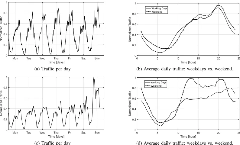
Fig. 1 shows the downlink aggregated throughput of two eNodeBs averaged over the 30 days of monitoring. We can distinguish the traffic per week in Fig. 1 a) and c) and the daily traffic in Fig. 1 b) and d).

A strong relation between mobile traffic and con-nected users is recognized. We observe the same daily pattern repetition: high traffic is shown during the hours of the day (when population is active), whereas less intensive traffic is experienced during nights (when people sleep). Traffic intensity is similar in working days and during weekends. A different behavior is detected in one particular cell, where a higher traffic is normally experienced on Sunday (Fig. 1 c) and d)). The reason behind this higher activity, is the presence of a local market open every Sunday in the same area where the eNB is located. As for the connected users, the minimum traffic is around 5.30 am for all the cells; a more prominent peak can be seen around at 8

Mon Tue Wed Thu Fri Sat Sun

Time [days] 0

0.2 0.4 0.6 0.8 1

Normalized Traffic

(a) Traffic per day.

0 5 10 15 20 25

Time [hour]

0 0.2 0.4 0.6 0.8 1

Normalized Traffic

Working Days Weekend

(b) Average daily traffic: weekdays vs. weekend.

Mon Tue Wed Thu Fri Sat Sun

Time [days] 0

0.2 0.4 0.6 0.8 1

Normalized Traffic

(c) Traffic per day.

0 5 10 15 20 25

Time [hour]

0 0.2 0.4 0.6 0.8 1

Normalized Traffic

Working Days Weekend

(d) Average daily traffic: weekdays vs. weekend.

pm. The maximum ratio between the peaks observed in the measurements is 13.3. The absolute values of the traffic are different and depend on the location of the area where the eNodeB is deployed. Fig. 2 shows the normalized average daily traffic distribution of the observed cells. Also in this case, the daily average traffic profiles are similar in shape for all the cells, especially during low load period.

As a proof of representiveness of our measurements, we compare the extracted information from the col-lected data with the traffic model presented in the EU ICT FP7 EARTH [8]. The data used in this project are provided by a network operator. We observe that, considering a daily average, the two traffic shapes are compatible and very similar (see Fig. 2). This comparison does not account for the absolute values of the traffic, which are dependant on the location of the specific base station, but it shows, on average, how the traffic demand is distributed over 24 hours. A different coefficient for the traffic magnitude can be calculated for each eNodeB based on the active population of that zone.

0 5 10 15 20 25

Hour in a day [h]

0 0.2 0.4 0.6 0.8 1

Normalized traffic cell 1

cell 2 cell 3 cell 4 EARTH

Fig. 2: Normalized daily traffic of different LTE cells and EARTH model.

Next, we show some example statistics for the traffic intensity of the four observed cells. Fig. 3 and 4 show the probability density function (pdf) and the cumula-tive distribution function (cdf) by applying the Kernel Smoothing algorithm on the empirical data traces. We have computed the pdfs and cdfs for different periods of one day (slots of 1 hour duration) and we have also evaluated their variation during the day. The figure shows only 6 slots for the sake of simplicity. The numbers report the start/end hour of the day of the respective slot.

We notice that night and early morning are the periods with lower traffic intensity (slot 0-1 and slot 4-5 have curves on the left side of the graph). After that and till slot 20-21, the traffic is increasing (the curves are more on the right side of thexaxis). Moreover, we can identify that the curves for slot 8-9 and slot 12-13 are similar, which indicates that the traffic in those hours is almost at the same level.

0 0.1 0.2 0.3 0.4 0.5 0.6 Normalized traffic

0 5 10 15 20 25 30

PDF

slot: 0-1 slot: 4-5 slot: 8-9 slot: 12-13 slot: 16-17 slot: 20-21

Fig. 3: PDF of the eNodeB traffic for six 1 hour-duration time-slots of a day.

0 0.1 0.2 0.3 0.4 0.5 0.6 0.7 Normalized traffic

0 0.1 0.2 0.3 0.4 0.5 0.6 0.7 0.8 0.9 1

CDF

slot: 0-1 slot: 4-5 slot: 8-9 slot: 12-13 slot: 16-17 slot: 20-21

Fig. 4: CDF of the eNodeB traffic for six 1 hour-duration time-slots of a day.

Fig. 5: Connected users per cell.

Fig. 6: Connected users per cell - comparison.

5 10 15 20 25 MCS

0 0.2 0.4 0.6 0.8 1

Aggregated Traffic

cell 1 cell 2 cell 3 cell 4

(a) Total aggregated traffic

5 10 15 20 25

MCS 0

0.2 0.4 0.6 0.8 1

Average Traffic per Comm.

cell 1 cell 2 cell 3 cell 4

(b) Average traffic per communication

Fig. 7: Traffic associated to different MCS (aggregated vs. average).

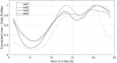
it is deployed in the centre of the city with a high population density and activity. However, normalizing the curves with respect to the daily maximum number of users, the same pattern is identified for all the cells (Fig. 6). The identified pattern follows a very similar behavior of the traffic profile. This confirms the correlation between the number of users and their generated traffic with the daily human activity.

B. Spatial behavior

We are able to estimate the quality of the channel experienced by the users during the communication with the eNodeB, based on the Modulation and Coding Scheme (MCS) assigned. One of the 28 possible MCS indexes is allocated by the eNodeB as a function of the Channel Quality Indicator (CQI) sent by the UE. The CQI depends on the SINR experienced by the user, which, among other factors, generally decreases with the distance between the eNodeB and the UE. In [9] a mapping between SINR values and different CQIs is provided. As a result of that, and based on the information on the assigned MCS, we estimate a spatial distribution of the user and combine it with the served traffic, in order to obtain a traffic distribution in space for each eNodeB.

Considering all the communications occurred in the recording period, Fig. 7a shows the aggregated amount of traffic for each assigned MCS index: the top three indexes are9, 10and11and this is confirmed for all the analyzed base stations. On the other hand, we see different profiles (Fig. 7b) when we consider only the average traffic per communication. This is due to the fact that the MCS indexes assigned by the eNodeB among the users are not uniformly distributed. For cell 1, except for the highest 3 MCS indexes, the users that experience a better quality of the channel also produce larger amount of traffic on average. However, a different behavior is noticed for cell 3: here, the largest communications correspond to a MCS index between

10and15.

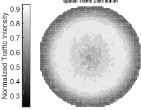
In Fig. 8, we analyze more than 10 millions com-munication traces between the eNodeB and the users. This map shows the spatial distribution of the users’ communications and the relative amount of traffic. Considering a cell in the center of the plot, the dis-tance between the users and the eNodeB is distributed according to the average MCS experienced during the communication. The exact angular position of the user is unknown and it is picked from a uniform distri-bution. The total amount of traffic produced during the communication gives the magnitude, represented by the different traffic intensities in the figure. The contour lines in the map group the areas with similar traffic distribution and highlight those that produce the larger amount of traffic. The groups shown in the figure demonstrates that the central region of a cell is usually the most dense and produce most of the traffic.

Spatial Traffic Distribution

0.3 0.4 0.5 0.6 0.7 0.8 0.9

Normalized Traffic Intensity

Fig. 8: Spatial traffic distribution of more than 10 million traces for a single eNodeB.

IV. DISCRETE-TIMEMARKOVTRAFFICMODEL

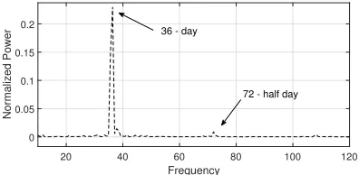
The proposed model aims at profiling the traffic pattern of a cell during a day. The daily time-scale has been selected based on the study of the frequency domain shown in Fig. 9, which reports a strong peri-odicity of the traffic during the 24 hours.

20 40 60 80 100 120 Frequency

0 0.05 0.1 0.15 0.2

Normalized Power

36 - day

72 - half day

Fig. 9: Periodogram of a 36 days-long traffic trace.

states. Formally, we consider a traffic intensity in bit per second during a given hour of the day, which can be in any of the statesxs∈ S={0,1, ..., Ns−1}. Every time step, the system evolves from a statexs(tk)to the next statexs(tk+1)∈ S according to the probabilities

puv(k) = P rob[xs(tk+1) = v|xs(tk) = u], with

u, v ∈ S, which is not null only if tk+1 = (tk+ 1)

modNt, beingNt the number of time slots in a day. To calculate the one-step transition probabilities from empirical data, we use Algorithm 1: for each step, the algorithm computes the transition probability matrix by counting how many times the cell traffic moves from a state to another. We obtain the correspondent probability matrix by normalizing each row.

Algorithm 1Transition Probability Matrix Calculation

1: procedure MARKOVMATRIX(data, Nt, Ns)

2: qData←quantizedatainNs levels

3: fortk in[0, ..., Nt−1]do

4: forx1in[0, ..., Ns−1]do

5: forx2 in[0, ..., Ns−1]do

6: Mx1,x2,tk ← count # transitions

xs1→x2 inqData(tk)

7: normalize rows ofM

8: returnM

V. NUMERICALRESULTS

In this section, we show some results on the stochas-tic Markov model for the daily traffic intensity. To evaluate our model, we split the dataset of a given cell into a training set and a validation set. The training set comprises 75% of the recording days and it is used to obtain the model through the presented algorithm. The validation set is used to have a numerical comparison with the traffic generated with the model.

Fig. 10 shows the error due to the selection of the number of states Ns and the number of slots

Nt. We apply a uniform quantization strategy that achieves accurate results, as demonstrated next. The error is calculated with respect to the validation trace as the average absolute daily difference, given by the following equation:

Err =

1

Ns NXs₋1

i=0

|xsim−xval| (1) We notice that an increase inNsandNtcorresponds to a decrease of the error. In particular, withNs ≥6 states andNt≥24time-slots, the error is small enough to produce a good approximation of the mobile traffic.

0 5 10 15 20 25 30 35 40 Nt

0.05 0.1 0.15 0.2 0.25 0.3 0.35 0.4

Average Daily Percentage Error

N_s = 2 N_s = 4 N_s = 6 N_s = 8 N_s = 10

Fig. 10: Error experienced changing the number of statesNs and the number of time-slotsNt.

Fig. 11 shows a 10-days synthetic traffic trace versus the validation dataset and their daily average, using

Ns= 10andNt= 24. We can see that, considering a sufficient number of days, the model is able to estimate with high accuracy the daily traffic pattern (Fig. 12).

0 2 4 6 8 10

Time [days] 0

0.1 0.2 0.3 0.4 0.5 0.6

Normalzed traffic

Original data Simulated data

Fig. 11: Simulated Traffic vs Original Data withNt=

24andNs= 10- 10 days.

0 5 10 15 20 25

Time [h] 0

0.1 0.2 0.3 0.4

Normalzed traffic

Original data Simulated data

Fig. 12: Simulated Traffic vs Original Data withNt=

24andNs= 10- Daily time scale.

traffic model. It shows the cdf of the synthetic traces applying the Kernel-Smoothing algorithm with the cdf of the traces from the validation set. We observe that the two curves almost overlap. Kolmogorov-Smirnov test is passed with a confidence of1%.

0 1 2 3 4 5

Traffic Rate [Mb/s] 0

0.2 0.4 0.6 0.8 1

CDF

Simulated Original

Fig. 13: CDFs of the synthetic traffic trace vs empirical traces.

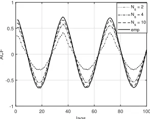
Finally, our Markov modelling approach is sufficient to accurately represent second-order statistic. Fig. 14 shows the autocorrelation function (ACF) for different values ofNs. With only 2-states (Ns= 2) the model is able to capture the periodicity of the traffic profiles and classify it in high or low load periods. However, major accuracy requires higher values ofNs. With Ns= 10 the model already performs satisfactorily. The good fit of the autocorrelation function confirms that, for a sufficient value of Ns, a further level complexity is unnecessary in the characterization.

0 20 40 60 80 100

lags -1

-0.5 0 0.5 1

ACF

N_s = 2 N_s = 4 N_s = 10 emp

Fig. 14: Autocorrelation function for the simulated traces and the empirical data for different values of

Ns.

VI. CONCLUSIONS

In this paper we have analyzed real mobile traffic traces with a tool, which is able to collect LTE down-link control channel in a reliable way. Through the collected data, we have obtained temporal and spatial characterization of the traffic of a mobile network. In addition, we have used this information to derive a stochastic characterization of the traffic using a discrete-time Markov chain. The numeric results prove

that the presented model represents a good fit for the empirical dataset: first and second order statistics show that the accuracy is sufficiently high with a limited number of states already.

ACKNOWLEDGEMENT

The research leading to this work has received funding from the Spanish Ministry of Economy and Competitiveness under grant TEC2014-60491-R (5GNORM) and from the European Union Horizon 2020 research and innovation programme under the Marie Skodowska-Curie grant agreement No 675891 (SCAVENGE).

REFERENCES

[1] I. Chih-Lin, C. Rowell, S. Han, Z. Xu, G. Li, and Z. Pan,

“To-ward green and soft: a 5g perspective,”IEEE Communications

Magazine, vol. 52, no. 2, pp. 66–73, 2014.

[2] V. D. Blondel, M. Esch, C. Chan, F. Cl´erot, P. Deville, E. Huens, F. Morlot, Z. Smoreda, and C. Ziemlicki, “Data for

develop-ment: the d4d challenge on mobile phone data,”arXiv preprint

arXiv:1210.0137, 2012.

[3] N. Bui and J. Widmer, “Owl: a reliable online watcher for lte

control channel measurements,”ACM All Things Cellular, 2016.

[4] F. Xu, Y. Li, H. Wang, P. Zhang, and D. Jin, “Understanding mobile traffic patterns of large scale cellular towers in urban

environment,”IEEE/ACM Transactions on Networking, 2016.

[5] OpenSignal.com, “https://opensignal.com/reports/,” 2017. [6] N. Bui and J. Widmer, “Data-driven Evaluation of Anticipatory

Networking Optimization on LTE Networks,” in submitted to

IEEE Transactions on Mobile Computing, 2017.

[7] ETSI, “E-UTRA; Physical channel and modulation,”3GPP TS,

vol. 36.211, p. V13, 2016.

[8] G. Auer, O. Blume, V. Giannini, I. Godor, M. Imran, Y. Jading,

E. Katranaras, M. Olsson, D. Sabella, P. Skillermark, et al.,

“Earth deliverable d2. 3: Energy efficiency analysis of the ref-erence systems, areas of improvements and target breakdown,” 2013.

[9] M. T. Kawser, N. I. B. Hamid, M. N. Hasan, M. S. Alam, and M. M. Rahman, “Downlink snr to cqi mapping for different

multipleantenna techniques in lte,” International Journal of

Information and Electronics Engineering, vol. 2, no. 5, p. 757,