Static Learning Particle Swarm Optimization with
Enhanced Exploration and Exploitation using
Adaptive Swarm Size
Aditya Panda1 ([email protected]), Srijan Ghoshal1([email protected]), Amit Konar1([email protected]), Bonny Banerjee2([email protected]), Atulya K Nagar3([email protected])
1
Dept. ETCE,Jadavpur University,Kolkata 70032,India,2 Electrical and Computer Engineering Department,University of Memphis,3815, Central Ave, Memphis, TN 38152, USA,3 Liverpool Hope University, Hope Park, Liverpool, L16 9JD. UK.
Abstract: In this paper, a novel Static Learning (SL) strategy
to adaptively vary swarm size has been proposed and integrated with Particle Swarm Optimization algorithm. Besides, the whole population has been divided into two sub swarms, where particles of different sub swarms interact within their neighbourhood and the existence of better particle is determined by evaluating its survival probability. Proper resource based particle replacement scheme and a linear chaotic term has also been included to ensure preservation of diversity of the swarm. In addition, the PSO algorithm is divided into two phases, with relevant algorithmic modification for each phase. The first phase is assigned to focus solely on better exploration of the search space. The second phase focuses on better utilization of the explored information. The proposed Static Learning Particle
Swarm Optimization with Enhanced Exploration and
Exploitation using Adaptive Swarm Size (SLPSO) algorithm is tested on a set of shifted and rotated benchmark problems and compared with six other recent state-of-the-art PSO algorithms. The proposed (SLPSO) algorithm demonstrates superior performance over other PSO variants.
Keywords: Static learning, exploration, exploitation, particle swarm optimizer.
I. INTRODUCTION
Since its inception, complexity of real parameter optimization problem has increased manifold. Researchers over the last decadehave improvised evolutionary algorithms to address these complex problems. These efforts includes Particle Swarm Optimization (PSO)[1], Differential Evolution (DE)[2], Ant Colony Optimization(ACO)[3], Artificial Bee-Colony(ABC)[4] etc. But Particle Swarm Optimization has attracted the attention of researchers as it outperforms other evolutionary algorithms in terms of simplicity and requirement of less number of parameters. However, a few drawbacks against PSO are that, it suffers from premature convergence around local maximadue to quick loss of diversity, stagnation of particle and oscillation around a local optimum.
Optimization through evolutionary algorithm solely depends on better exploration and exploitation of the search space. Even though there is difference in objective of these two phases, still most of the improved PSO reports, envisagesimplementation of the same algorithm for both the phases. In [5], Lynn et al. attempted to address this issue by
bifurcating the swarm into two parts with respectively assigned jobs for each sub swarm. Chen and Zhao in Ladder-type PSO (LPSO) [6] proposed periodical population renewal mechanism by dividing the swarm into equal periods called ladder. Increment or reduction in population size is designed by estimating diversity at the end of each ladder. Population size within each ladder is kept fixed. Leong et. al. in [7]have considered particles from non-dominated set to have higher probability of generating new particles that will improve the convergence toward the Pareto front. Random number of particles from the non-dominated set is selected as parent particle. The number of particles to be generated from each parent particle is selected by evaluating an adaptive probability. Tan et. al. [8] also considered adaptive swarm size to adjust the swarmsize- based on an approximate tradeoff of the hyper-area already discovered by the swarm and taking experience from the dominant particles or leader particles. These efforts,though include adaptive swarm size, but the same algorithm has been used for both exploration and exploitation stage.
In this paper, we have tried to mitigate the gap by employing two different improved algorithms for two phases. The swarm completely focuses on exploration in the first phase and at the end of this phase, each optimum contains at least one particle. Exploration being over, the swarm switches to next phase to exploit the explored information. A novel static learning strategy based on multi variable regression, has been proposed, which helps the particle to learn from the explored knowledge in first phase and adaptively vary its swarm size. In the exploration phase, proper diversity enhancement has been ensured by particle replacement scheme and with addition of linear chaos.
II. STANDARD PSO, A BRIEF OVERVIEW:
Inspired by bird flocking and fish swarming, Kennedy and Eberhart in 1995 [1] introduced a population based stochastic search algorithm, Particle Swarm Optimization (PSO), aimed at obtaining optimal solution for complex non-linear optimization problems. In PSO, particles are taken to be pseudo entities having position and velocity. The position of each particle is a potential solution to a given optimization problem. Originally, PSO was designed for real-valued optimization problems. Later it was extended for binary and linear optimization problems, too. The first version of PSO, called gbesttopology, considered the personal and the global best experiences of the particles to determine their next positions. The gbest algorithm has a faster convergence but is more susceptible to getting trapped into local optima. However, Kennedy in [9] reported lbest PSO, where the best position of a particle in the neighborhood is considered instead of the entire population. lbest topology with small neighborhood performs better on complex multimodal surfaces, while PSO with a large neighborhood is preferred for optimization of unimodal functions. Different topological neighborhoods have emerged, over the years, which are basically connected graphstructures. Among them, ring neighbourhood is the most popular. In this paper, for each particle, the sub swarm to which it belongs to is taken as its neighborhood.
PSO algorithm emulates thenatural model of social and cognitive co-operation, where each particle’s trajectories are guided by its personal best experience as well global best experience. For a N particle swarm, the velocity of ithparticle, where i ∈{1,2, . . }is given by Kennedy and Eberhart[1] as
⃗( + 1) = ⃗( ) + ∗ 1 ∗ _ ⃗( )− ⃗( ) + ∗
2 ∗ _ ⃗( )− ⃗( ) , (1) The position update expression is given by,
⃗= ⃗+ ⃗ (2)
where, ⃗(t), ⃗(t) are the velocity and position of the ith particle of the swarm at tth iteration. _ ⃗( ) and _ ⃗ global best and personal best positions for the ith particle for tth iteration, respectively. and are acceleration coefficients and 1 and 2 are random numbers 1, 2 ∈[0,1]. In [10] balance between global and local topology has been done, with introduction of inertia weight ω in the velocity update expression, represented as,
⃗( + 1) = ∗ ⃗( ) + ∗ 1 ∗ _ ⃗( )− ⃗( ) +
∗ 2 ∗ _ ⃗( )− ⃗( ) (3)
In 1999, analyzing swarm dynamics of PSO, Clerc and Kennedy [11][12], further proposed another parameter, constriction coefficient , to restrict the velocity of particles,represented by the following expression,
← ∗[ ∗ ⃗+ ∗ 1 ∗ _ ⃗ − ⃗ + ∗
2 ∗ _ ⃗ − ⃗ ], (4)
Where χ is the constriction coefficient represented by the following expression,
=
| | , where = c1+ c2and > 4
Recent algorithmic improvements in PSO include the Fully Informed Particle Swarms (FIPS) [15], suggested by Mendes et al., where a particle gets knowledge from its own neighbourhood as well as other neighbourhood. In Comprehensive Learning Particle Swarm Optimization (CLPSO) [14] Liang et al. used a comprehensive learning strategy where each particle can learn from its own personal best as well as other particle’s other dimension’s personal best experiences. In [16], Suganthan et al. reported Dynamic Multi Swarm Particle Swarm Optimization (DMSPSO) where the swarm was decomposed into multiple sub swarms where each sub swarm learns from its own sub swarm as well as other sub swarms. Zhang et al. suggested Orthogonal Learning Particle Swarm Optimization (OLPSO) [17], where the Orthogonal Learning strategy (OL) was integrated with PSO.
.
IIITHE PROPOSED SLPSOALGORITHM
Standard PSO utilizes the same algorithm for exploration and exploitation without any proper demarcation. The proposed SLPSO algorithm has been separated into two phases. The first phase is exclusively for exploration of the solution space, while in the second phase more focus is given on better exploitation of the knowledge already explored about the search space. Specific algorithmic modifications have been done to uniquely assign the job of exploration to one phase and the job of exploitation to another phase.
A. The exploration phase
One of the major requirements in the first of optimization is, exploring the search space maintaining diversity in the swarm, to prevent premature trapping around local optima. In the proposed SLPSO algorithm, at the beginning, half of the swarm is randomly assigned to subgroup A and the next half of the swarm to subgroup B. Information sharing has been restricted to introduce competition between the two sub swarms. Accordingly, each of the sub swarms, in this phase is updated by influence from its personal best experience as well as the leader of its own sub swarm. For ithparticle belonging to kth sub swarm, the update expression can be given as,
⃗( + 1) = ∗ ⃗( ) + ∗ 1 ∗ _ ⃗( )− ⃗( ) + ∗ 2 ∗ _ ⃗( )− ⃗( ) (5)
where _ ⃗( ) is the leader or best position explored by kth sub swarm in titerations.
After a refreshing gap of m iterations, Euclidian distance between each pair of particle is evaluated. To restrict the premature convergence, a ϵ neighbourhood is defined around each particle. When two or more particles come within the same ϵ neighbourhood, then for each particle, “Survival Probability”, Pis evaluated as,
=
∑ , whereN isthesizeofthesubswarm
Among all the particle within the same neighbourhood, the particle with the highest “Survival Probability” from each subgroup survives and to protect diversity, rest of the particles are deleted, as they represent repaetation of same information. Since the local best particle from both sub swarms are kept, it ensures that the local optimum is not completely lost from the swarm. The selection of the used expression for survival probability can be well justified from nature’s principle of ‘survival of the fittest’. Since for an optimization problem, ‘fitness’ is the most significant resourse, while multiple particles fightes for the same resourse, the fittest particles ultimately wins the conflict i.e. it is assigned higher chance to survive. In addition, as denominator aggregates the sub swarm finesses, not the whole swarm fitness, reported strategy selects better representative from each sub swarm only.
Now after deletion of particles, the swarm size will be reduced, which is not expected in the exploration stage. Therefore, to increase the population size to its original size, we add particles using a novel ‘Position Reflection’ strategy. When a particle belonging to asub swarm is deleted, the created particle is added to the other sub swarm. This replicates natural models of competition for finding resource, the unfit sub swarm gets weakened and the fit sub swarm strengthened.The replacement using position reflection strategy primarily focuses on exploration of unexplored areas to increase diversity of the swarm. For each deleted particle a temporary location is generated by rule specified by the expression stated below,
x ⃗= 2∗ x ⃗ − μ ⃗ ⃗ (7)
Two random particles are selected from the swarm as parent elements and µ is a random number, µ ∈ [0,1].
Fig. I. Position reflection rule
B. Effect of chaos
Chaos is a state of disorder that introduces some sort of uncertainty in the system and as a result of it, the behaviour of the particle deviates from its deterministic nature specified by conventional iterative equation. In the proposed SLPSO algoirithm, chaos represented as ∆⃗=∑ ∗ (0,1) , has been added velocity of the particle to increase the non deterministic behaviour in swarm trajectory. When a particle gets trapped in a local optimum, the chaos term may help to come out of the trap and eventually prevent premature convergence. The velocity update expression can be modified as,
⃗( + 1) = ⃗( ) + ∗ 1 ∗ ⃗( )− ⃗( ) + ∗ 2 ∗ ⃗( )− ⃗( ) +∑ ∗ (0,1) (8)
where is jth dimension unit vector and is jth dimension of velocity for ith particle.
C. Switching from exploration phase to exploitation Phase
The primary focus for exploration phase was to searching for optima while maintaining diversity. When the diversity is greater than certain threshold value ( ) then we conclude that the swarm has gained sufficient information about the search space and the algorithm switches to exploitation phase. Further if due to random initialization, if at the very beginning D≥ is satisfied then too we run exploration phase for a few steps to gain sufficient information for the search space from which the algorithm can learn in exploitation phase.Diversity of the swarm is evaluated at the end of an integral multiple of refreshing gap, by using the following formula
Diversity(D) = ∑ ⃗ ⃗
∑ ( ⃗ ⃗)
where,⃗ =( ⃗ ⃗)
(9)
where ‖ ⃗ ‖ denotes the eucledian norm for ⃗. The denominator defines the maximum allowable deviation for any particle and the numerator defines its deviation from the
central position, i.e. ⃗ =( ⃗ ⃗),evidently 0≤ ≤1.
D. The exploitation phase
In this phase, the swarm exploits the information already explored in first phase. After the exploration phase, the swarm is more or less scattered only around the potential optima on the solution space. Now the swarm should converge to one peak solution. Hence, the swarm size is adjusted according to the dependency on relevant parameters and we try to model the dependencies based on the following propositions.
Proposition 1: The sub swarm, which contains better fitness values, should be encouraged to expand in strength as it may possess potential solutions. Therefore, average fitness can be considered as a control parameter for sub swarm size.
=
( ) = ( )(10)
Proposition 2: In the exploitation sub phase, convergence of the swarm around potential optimum is desired. Hence, the sub swarm with more compact particles has better chances of converging around potential solution. Therefore, if the second order moment of the position of all the particles about the sub swarm best position in a particular sub swarm is more, it is more dispersed, which is detrimental to convergence. So, second order moment of position can be treated as one of the parameters in the exploitation phase.
− = ( ℎ
ℎ ℎ
Fig. II: State I & state II in the second proposition of exploitation phase
Proposition 3: Considering multi swarm algorithm, all the sub swarms mustmerge to one central maximum and hence the sub swarm, furthest from other potential sub swarms should decrease in size. Mathematically, we can consider second order moment of the mean position of all the particles about fittest sub swarm’smean position in the optimization space thus it becomes an important parameter for exploitation phase.
− = ( ℎ
ℎ ℎ
)= ( ) (12)
Fig. III: State I & state II in the third proposition of exploitation phase
The mean position of kth sub swarm is calculated as, ⃗=
∑ ⃗
, and distance from fittestsub swarmis calculated as,
= ⃗ − ⃗ (13)
Combining all of the three propositions (considering identity relation i.e. f(x) =x), we construct expression for rate of change of swarm size for exploitation phase with respect to iterations as, for j sub swarm (j=A or j=B),
= − − (14) where x is taken as average itnees value,y denotes standard deviation with respect to the position of the particle in a swarm and z represents 2nd order moment of distance of other sub swarms from the sub swarm under consideration. In
discrete domain, we have, = ( ) ( )
( ) =∆ ,which implies, ∆ ( + 1) = ( )− ( )− ( ). If ∆ >0 we propose the addition of particles to encourage convergence by intense fine search in and around each particle. Three parent particles are randomly selected from the swarm as,
⃗ = ⃗ ⃗ ⃗ (15)
where, a and b are random numbers a,b ∈[0,1], c=3-(a+b); On the other hand if ∆ <0 to protect swarm fitness values we delete the poorest ∆ number of particles. Here the flow information is not restricted and particles share from each other’s information too.
E. Estimation of the parameters α, β and λ through static
learning strategy:
In Exploration phase, we have varied the size of the two sub swarms according to fitness achieved by them. After each refreshing gap of a few iterations,sizes of respective sub swarms have changed and we calculate the values ofx,y , z. These data setsX = {x , x , … x },Y = {y , y , … y }, Z = {z , z , … z }are utilized to estimate the parameters using regression on multiple data sequences. The process is briefly described below.
∆ = − −
∆ = − −
…….
∆ = − −
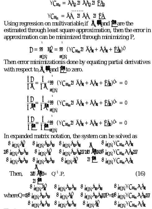
Using regression on multivariable,if , and are the estimated through least square approximation, then the error in approximation can be minimized through minimizing P,
= = (∆ − + + )
Then error minimizationis done by equating partial derivatives with respect to, , and , to zero.
= (∆ − + + ) = 0
= (∆ − + + ) = 0
= (∆ − + + ) = 0
In expanded matrix notation, the system can be solved as
∑ ∑ ∑
∑ ∑ ∑
∑ ∑ ∑
. − −
=
∑ ∆ ∗
∑ ∆ ∗
∑ ∆ ∗
Then, − −
= Q-1 .P, (16)
whereQ=
∑ ∑ ∑
∑ ∑ ∑
∑ ∑ ∑
,P=
∑ ∆ ∗
∑ ∆ ∗
∑ ∆ ∗
F. The Pseudo code for the proposed algorithm:
Algorithm: High-level pseudo-code of the proposed SLPSO algorithm
Input: Swarm size N, No of dimensions D, Maximum allowed generations for the optimization MAX_IT, Refreshing Gap m. Output: final global best vector
Begin:
1. Randomly initialize positions and velocity for each particle 2. Randomly divide the particles into two sub swarm 3. while (t<=MAX_IT) do
// exploration
4. while Diversity≤ do
5. for i← 1 to N do
6. for j← 1 to D do
7. if i∈
8. Vi← ω*Vi + c1*rand(0,1)*(swarm_best - xi)+ c1*rand(0,1)*(personal best - xi)+∆=∑ 1 ∗ (0,1)
9. elseif i∈
10. Vi← ω*Vi + c1*rand(0,1)*(swarm_best - xi)+ c1*rand(0,1)*(personal best - xi)+∆=∑ 1 ∗ (0,1)
11. endif
12. Xi← Vi+ Xi
13. endfor
14. update personal best,swarm_best and swarm_best
15. if t ==integral multiple of m do
//prevent premature convergence
16. for i← 1 to N do
17. for j← (i+1) to N do
18. if − <∈ do
19. for all particles within the same neighborhood, evaluate
=
∑ ,whereNAisthestrengthofthesubswarminwhichi
thparticlefalls
20. delete all the particles except the particle highest P
21. add particles corresponding to each deleted particle according to expression (7)and assign them to the other sub group
22. endif
23. endfor
24. endfor
25. endif
endfor t← t +1
26. endwhile
27. //exploitation
28. estimate the least square approximation of the α,βand λ parameters
29. estimate the ∆ ∆
30. if ∆ >0
31. add particles according to expression (15)
32. elseif ∆ <0
33. delete weakest ∆ particles from sub swarm A
34. endif
35. if ∆ >0
36. add particles according to expression (15)
37. elseif ∆ <0
38. delete ∆ particles from sub swarm B
39. endif
40. for i← 1 to N
41. for j← 1 to D do
42. if i∈
43. Vi← ω*Vi + c*rand(0,1)*(swarm_best - xi)+ c*rand(0,1)*(personalbest - xi)
44. elseif i∈
45. Vi← ω*Vi + c*rand(0,1)*(swarm_best - xi)+ c*rand(0,1)*(personalbest - xi)
46. endif
47. endfor
48. Xi← Vi+ Xi
49. endfor
t← t +1
IV Experimental Results
A. Experimental setup:
Results are tested and compiled on 25 benchmark function in IEEE Congress on Evolutionary Computations 2005 (CEC 2005) test bed as suggested by suganthan et. al.[13]. All the benchmark functions are listed below with their respectivefunction types.
TABLE I. THE CEC2005BENCHMARK FUNCTION
Function No.
Function name Function
type F1 Shifted Sphere Function
Unimodal Function F2 Shifted Schwefel’s Problem 1.2
F3 Shifted Rotated High Conditioned Elliptic Function
F4 Shifted Schwefel’s Problem 1.2 with Noise in Fitness
F5 Schwefel’s Problem 2.6 with Global Optimum on Bounds
F6 Shifted Rosenbrock’s Function
Multimodal Function F7 Shifted Rotated Griewank’s Function without
Bounds
F8 Shifted Rotated Ackley’s Function with Global Optimum on Bounds
F9 Shifted Rastrigin’s Function F10 Shifted Rotated Rastrigin’s Function F11 Shifted Rotated Weierstrass Function F12 Schwefel’s Problem 2.13
F13 Expanded Extended Griewank’s plus Rosenbrock’s Function (F8F2) F14 Shifted Rotated Expanded Scaffer’s F6 F15 Hybrid Composition Function
Hybrid Composition Function Hybrid Composition Function F16 Rotated Hybrid Composition Function
F17 Rotated Hybrid Composition Function with Noise in Fitness
F18 Rotated Hybrid Composition Function F19 Rotated Hybrid Composition Function with a
Narrow Basin for the Global Optimum
F20 Rotated Hybrid Composition Function with the Global Optimum on the
Bounds
F21 Rotated Hybrid Composition Function F22 Rotated Hybrid Composition Function with
High Condition Number Matrix F23 Non-Continuous Rotated Hybrid
Composition Function
F24 Rotated Hybrid Composition Function F25 Rotated Hybrid Composition Function
without Bounds
B. Parameter selection
The size of the proposed ϵ neighbourhood is decreased linearly throughout the iterations. This is done in accordance with accommodate more particles around each optima near the termination of the algorithm to allow finer search.
ϵmax=0.01* ⃗ − ⃗ (17)
and ϵ= ϵmax- ϵmax*
_ (18)where t is the current iteration. Threshold diversity is taken to be
0.9. Refreshing gap m is taken constant at 7 iterations. Inertia weight, ω is taken to be fixed at ω=0.729 and C1=
C2=1.494. MAX_FE is taken in accordance with the IEEE
CEC 2005 guidelines as 10,000*D and for the 10 Dimensional function, it is taken as 1 Lakh FEs. Initial swarm size or population size is taken to be 50. Codes were implemented in Matlab R2011a release, and executed on intel i5 3.00 GHz CPU and 4GB RAM on Microsoft Windows 7 operating system. Each function is run for 15 independent runs and the result is therefore averaged.
C. Compared algorithms:
Proposed SLPSO algorithm is compared with 5 other state-of-the-art algorithms,PSO[1], FIPS[11], DMSPSO[12], CLPSO[10], OLPSO[13]. And the results are compiled and compared. Parameters for compared algorithms are taken same as reported by respective authors in the original literatures.
V Experimental Results and Discussions
A. Results:
Proposed Algorithm is compared with five otherPSO algorithmsand result is tabulated below.
TABLE II. RESULTS AND COMPARISON WITH PSO, FIPS AND DMSPSO
Algo Func
SLPSO PSO FIPS DMSPSO
F1 Mean Std. Rank 0.00E+00 0.00E+00 3.5 0.00E+000. 00E+00 3.5 0.00E+00 0.00E+00 3.5 0.00E+00 0.00E+00 3.5 F2 Mean
Std. Rank 0.00E+00 0.00E+00 3 0.00E+00 0.00E+00 3 0.00E+00 0.00E+00 3 5.17E-08 0.00E+00 6 F3 Mean
Std. Rank 1.02E+05 4.68E+04 3 1.60E+05 1.10E+05 4 2.24E+05 1.22E+05 5 6.53E+04 1.36E+04 2 F4 Mean
Std. Rank 0.00E+00 0.00E+00 2.5 0.00E+00 0.00E+00 2.5 0.00E+00 0.00E+00 2.5 1.34E+01 1.20E+00 6 F5 Mean
Std. Rank 1.01E+03 2.23E+02 4 1.04E+03 2.07E+02 5 1.32E+02 1.11E+02 1 2.36E+02 4.31E+01 2 F6 Mean
Std. Rank 1.79E-03 1.02E-06 1 3.47E+01 7.76E+01 5 4.70E+01 1.23E+01 6 1.34E+00 9.05E-02 3 F7 Mean
Std. Rank 7.14E-02 1.26E-05 1 2.32E+01 8.41E-01 6 2.31E+00 1.31E+00 5 1.24E-01 7.02E-08 2 F8 Mean
Std. Rank 2.02E+01 2.12E-01 1.5 2.19E+02 9.01E-02 5 2.08E+01 8.00E-02 3 1.35E+02 4.26E+01 6 F9 Mean
Std. Rank 1.23E+00 2.12E-01 3 3.55E+00 2.54E+00 4 2.34E-01 5.72E-01 1 1.25E+01 2.04E+00 5 F10 Mean
Std. Rank 1.33E+01 1.26E+00 2 2.44E+01 5.21E+00 5 1.43E+01 6.40E+00 3 1.47E+01 1.29E+00 4 F11 Mean
Std. Rank 1.64E+00 2.51E-01 2 3.36E+00 1.42E+00 3 4.55E+00 1.61E+00 5 1.04E+00 8.41E-01 1 F12 Mean
F13 Mean Std. Rank 4.94E-01 2.11E-01 2 1.72E+00 1.43E-01 6 1.17E+00 2.64E-01 4 1.24E+00 4.38E-01 5 F14 Mean
Std. Rank 2.69E+00 1.20E-01 1 3.86E+00 4.10E-01 5 2.93E+00 3.41E-01 2 1.26E+01 3.59E-01 6 F15 Mean
Std. Rank 3.34E+01 1.02E+01 1.5 3.34E+02 1.76E+02 6 2.08E+02 1.76E+02 4 3.34E+01 2.36E+001. 5 F16 Mean
Std. Rank 1.08E+02 4.23E+01 1 1.29E+02 1.64E+01 5 1.12E+02 9.91E+00 2 1.18E+02 2.59E+00 3 F17 Mean
Std. Rank 8.02E+02 2.28E+01 5 7.10E+02 2.53E+02 4 8.06E+02 1.34E+02 6 5.46E+02 2.32E+01 1 F18 Mean
Std. Rank 1.21E+02 1.32E+01 1 1.42E+02 6.81E+01 4 1.24E+02 1.46E+01 2 3.74E+02 8.56E+00 6 F19 Mean
Std. Rank 6.12E+02 1.23E+01 1 8.99E+02 2.45E+02 6 7.59E+02 1.69E+02 5 6.56E+02 4.32E+01 3 F20 Mean
Std. Rank 6.02E+02 1.32E+02 1 7.16E+02 2.66E+02 5 7.01E+02 1.35E+02 3 8.35E+02 1.28E+02 4 F21 Mean
Std. Rank 5.01E+02 4.64E+02 1 1.04E+03 2.83E+02 6 7.65E+02 2.84E+02 5 6.62E+02 2.32E+01 4 F22 Mean
Std. Rank 7.01E+02 2.23E+01 1 8.64E+02 9.30E+01 5 7.98E+02 6.13E+01 4 7.86E+02 4.23E+01 3.5 F23 Mean
Std. Rank 6.12E+02 3.66E+02 2 1.12E+03 1.43E+02 6 8.57E+02 2.66E+02 5 7.18E+02 1.27E+02 4 F24 Mean
Std. Rank 2.00E+02 1.34E-02 2 3.77E+02 1.56E+02 6 2.80E+02 3.90E+00 5 2.45E+02 1.46E+01 4 F25 Mean
Std. Rank 2.00E+02 1.04E-06 1.5 3.77E+02 1.75E+02 5 3.80E+02 2.33E+00 6 3.16E+02 2.86E+01 4 Avg. Rank. 1.86 1 4.68 6 3.92 5 3.78 4
TABLE III. RESULTS AND COMPARISON WITH CLPSO AND OLPSO
Algo Func
SLPSO CLPSO OLPSO
F1 Mean Std. Rank 0.00E+00 0.00E+00 3.5 0.00E+00 0.00E+00 3.5 0.00E+00 0.00E+00 3.5 F2 Mean
Std. Rank 0.00E+00 0.00E+00 3 1.86E-02 2.24E-02 5 0.00E+00 0.00E+00 3 F3 Mean
Std. Rank 1.02E+05 4.68E+04 3 3.94E+05 2.21E+05 6 6.36E+04 3.81E+04 1 F4 Mean
Std. Rank 0.00E+000 .00E+00 2.5 5.20E+00 1.12E+01 5 2.15E+00 2.96E+02 4 F5 Mean
Std. Rank 1.01E+03 2.23E+02 4 5.32E+03 1.23E+01 6 4.96E+02 3.61E+02 3 F6 Mean
Std. Rank 1.79E-03 1.02E-06 1 8.62E-01 1.63E+00 2 1.18E+01 2.20E+00 4 F7 Mean
Std. Rank 7.14E-02 1.26E-05 1 2.13E-01 1.41E-01 3 2.56E-01 1.84E+004
F8 Mean Std. Rank 2.02E+01 2.12E-01 1.5 2.14E+01 5.00E-02 4 2.02E+01 1.10E-01 1.5
F9 Mean Std. Rank 1.23E+00 2.12E-01 3 0.00E+000. 00E+00 2 1.76E+00 1.47E+00 5 F10 Mean
Std. Rank 1.33E+01 1.26E+00 2 9.24E+00 2.97E+00 1 3.00E+01 1.09E+01 6 F11 Mean
Std. Rank 1.64E+00 2.51E-01 2 4.53E+00 5.81E-01 4 5.91E+00 1.91E+00 6 F12 Mean
Std. Rank 1.30E+01 1.02E-02 1 7.22E+01 5.20E+01 4 5.70E+01 7.52E+05 3 F13 Mean
Std. Rank 4.94E-01 2.11E-01 2 2.73E-01 6.23E-01 1 6.61E-01 2.04E-01 3 F14 Mean
Std. Rank 2.69E+00 1.20E-01 1 3.00E+00 2.63E-01 3 3.20E+00 3.23E-01 4 F15 Mean
Std. Rank 3.34E+01 1.02E+01 1.5 4.81E+01 1.76E+01 3 2.15E+02 2.04E+02 5 F16 Mean
Std. Rank 1.08E+02 4.23E+01 1 1.20E+02 9.92E+00 4 1.91E+02 3.91E+01 6 F17 Mean
Std. Rank 8.02E+02 2.28E+01 5 6.85E+02 1.87E+02 2 7.01E+02 8.67E+013
F18 Mean Std. Rank 1.21E+02 1.32E+01 1 1.25E+02 1.29E+01 3 1.95E+02 4.47E+01 5 F19 Mean
Std. Rank 6.12E+02 1.23E+01 1 6.54E+02 1.88E+02 2 6.95E+02 9.26E+01 4 F20 Mean
Std. Rank 6.02E+02 1.32E+02 1 7.46E+02 1.62E+02 6 6.86E+02 1.12E+02 2 F21 Mean
Std. Rank 5.01E+02 4.64E+02 1 5.52E+02 1.40E+02 3 5.51E+02 1.93E+022
F22 Mean Std. Rank 7.01E+02 2.23E+01 1 7.27E+02 1.42E+02 2 7.86E+02 1.30E+02 3.5 F23 Mean
Std. Rank 6.12E+02 3.66E+02 2 5.58E+02 7.16E+01 1 6.77E+02 2.63E+02 3 F24 Mean
Std. Rank 2.00E+02 1.34E-02 2 2.00E+02 1.63E+01 2 2.00E+02 2.36E+02 2 F25 Mean
Std. Rank 2.00E+02 1.04E-06 1.5 2.00E+02 2.59E-09 1.5 2.37E+02 4.37E+01 3 Avg. Rank. 1.86 1 3.16 2 3.60 3
The ranks are shown in the following diagram:
Fig. IV: Rank comparison of different PSO algorithms
1.86 4.68 3.92 3.78 3.16 3.6 0 2 4 6
SLPSO PSO FIPS DMSPSO CLPSO OLPSO
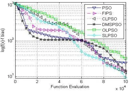
Fig. V: Convergence plot for F10
B. Discussion:
In this paper, a novel modification of PSO was suggested and compared on the IEEE CEC 2005 testbed function. Very few literatures on PSO, has attempted to adaptively vary swarm size. In this article we have modeled the swarm size as a dependent parameter on the particular optimization search space. It was observed that SLPSO algorithm suggests very promising results for unimodal, multimodal, rotated and hybrid composition functions. However the algorithm fails for F17 which is ‘Hybrid composition Function withNoise’. Hence it can be concluded the proposed algorithm does not perform satisfactory with noisy functions. The failure may be due to the fact that, in case of noisy search space 2nd and 3rd degree dependencies in equation (14) need to be considered for clustering in the rough data space. The function does not perform satisfactory on F3, Shifted Rotated High Conditioned Elliptic Function. Also as dimensionality of the optimization increases, performance proposed algorithm decreases, which was observed to improve further if higher degree of dependency is considered in equation (14), as stated earlier. However as “No Free Lunch” theorem states that there cannot be any single optimization algorithm for all sets of optimization problems. Hence we conclude that the reported algorithm outperforms existing PSO algorithms in unimodal, multi modal, hybrid composition functions.
V Conclusion
In this paper the swarm size has been kept adaptive to the function space with specialized models for exploration and exploitation, and this suggested an improved results. The swarm size variation dependency was taken to be linear function of control parameters but it is matter of further research to investigate the degree dependency. For noisy and ill conditioned functions higher degree of dependencies must be used.
VI Acknowledgement
Dr. Bonny Banerjee was supported by NSF grant IIS-1231620
VIIReferences
[1] Eberhart R. C. and Kennedy J., “A new optimizer using particle swarm theory”, in Proc. 6th Int. Symp. Micromachine Human Sci. (MHS), Piscataway, NJ, 1995, pp. 39–43.
[2] Price K. et. al., “Differential Evolution: A Practical Approach to Global Optimization.” Berlin, Germany: Springer-Verlag, 2005. [3] Dorigo M, et. al. "Ant colony optimization." In Encyclopedia of
machine learning, pp. 36-39. Springer US, 2010.
[4] Karaboga, D, and Basturk B. "A powerful and efficient algorithm for numerical function optimization: artificial bee colony (ABC) algorithm." Journal of global optimization 39, no. 3 (2007): 459-471. [5] Lynn, N. and Suganthan P. N., "Heterogeneous comprehensive
learning particle swarm optimization with enhanced exploration and exploitation." Swarm and Evolutionary Computation 24 (2015): 11-24.
[6] Chen DeBao, and ChunXia Zhao. "Particle swarm optimization with adaptive population size and its application." Applied Soft
Computing 9.1 (2009): 39-48.
[7] Leong, Wen-Fung, and Gary G. Yen. "PSO-based multiobjective optimization with dynamic population size and adaptive local archives." Systems, Man, and Cybernetics, Part B: Cybernetics, IEEE
Transactions on 38.5 (2008): 1270-1293.
[8] Tan, K. C., T. H. Lee, and E. F. Khor. "Evolutionary algorithms with dynamic population size and local exploration for multiobjective optimization, vol. 5." (2001): 565-599.
[9] Kennedy J., “The particle swarm: Social adaptation of knowledge,” in
Proc. IEEE Int. Conf. Evol. Comput., Apr. 1997, pp. 303–308.
[10] Shi, Y., and Eberhart R. C. "A modified particle swarm optimizer." Evolutionary Computation Proceedings, 1998. IEEE World Congress on Computational Intelligence., The 1998 IEEE International Conference on. IEEE, 1998.
[11] Clerc, M. "The swarm and the queen: towards a deterministic and adaptive particle swarm optimization." Evolutionary Computation, 1999. CEC 99. Proceedings of the 1999 Congress on. Vol. 3. IEEE, 1999.
[12] Kennedy J., and Blackwell T., "Particle swarm optimization." Swarm intelligence 1.1 (2007): 33-57.
[13] Suganthan, Ponnuthurai N., et al. "Problem definitions and evaluation criteria for the CEC 2005 special session on real-parameter optimization." KanGAL report 2005005 (2005): 2005.
[14] Liang, Jing J., et al. "Comprehensive learning particle swarm optimizer for global optimization of multimodal functions." Evolutionary Computation, IEEE Transactions on 10.3 (2006): 281-295.
[15] Mendes, R, Kennedy J., and José N. "The fully informed particle swarm simpler, maybe better." Evolutionary Computation, IEEE
Transactions on 8.3 (2004): 204-210..
[16] Liang J. J. and Suganthan P. N., Dynamic multi-swarm particle swarm optimizer. in Proc. of IEEE Swarm Intelligence Symposium, 2005, pp. 124–129.