Determining The Optimal Values
Of Exponential Smoothing
Constants – Does Solver Really Work?
Handanhal V. Ravinder, Montclair State University, USAABSTRACT
A key issue in exponential smoothing is the choice of the values of the smoothing constants used. One approach that is becoming increasingly popular in introductory management science and operations management textbooks is the use of Solver, an Excel-based non-linear optimizer, to identify values of the smoothing constants that minimize a measure of forecast error like Mean Absolute Deviation (MAD) or Mean Squared Error (MSE). We point out some difficulties with this approach and suggest an easy fix. We examine the impact of initial forecasts on the smoothing constants and the idea of optimizing the initial forecast along with the smoothing constants. We make recommendations on the use of Solver in the context of the teaching of forecasting and suggest that there is a better method than Solver to identify the appropriate smoothing constants. Keywords: Exponential Smoothing; Smoothing Constants; Forecast Error; Non-Linear Optimization; Solver
INTRODUCTION
xponential smoothing is one of the most popular forecasting techniques. It is easy to understand and easy to use. Popular forecasting software products include it in their offerings. All graduate and undergraduate business students are taught exponential smoothing at least once in an operations management or management science course. Gardner (1985, 2006) provides a detailed review of exponential smoothing.
Exponential smoothing techniques are usually discussed in the context of three situations characterized by increasing complexity.
Simple Exponential Smoothing
Here, demand is level with only random variations around some average. The forecast Ft+1 for the
upcoming period is the estimate of average level Lt at the end of period t.
(1)
where α, the smoothing constant, is between 0 and 1. We can interpret the new forecast as the old forecast adjusted by some fraction of the forecast error. Equivalently, we can view the new estimate of level as a weighted average of Dt (the most recent information on average level) and Ft (our previous estimate of that level).
Lt (and Ft+1) can be written recursively in terms of all previous demand as:
(2)
Thus, Ft+1is a weighted average of all previous demand with the weight on Di given by α(1-α)t-i where t is the period
Exponential Smoothing with Trend Adjustment (Holt’s Model)
In this case, the time series exhibits a trend; in addition to the level component, the trend (slope) has to be estimated.
The forecast, including trend for the upcoming period t+1, is given by
(3)
Here, is the estimate of level made at the end of period t and is given by
(4)
is the estimate of trend at the end of period t and is given by
(5)
β is also a smoothing constant between 0 and 1 and plays a role very similar to that of α. Exponential Smoothing with Trend and Seasonality (Winter’s Model)
Here, the forecast for the upcoming period, t+1, is the sum of estimates of level and trend adjusted by a seasonality index for t+1. The level and trend relationships are much the same as in Holt’s model, except that level calculations are now based on deseasonalized demand in period t and estimate of level for period t. The seasonality index for the period just ended is revised on the basis of the observed demand and the most recent level estimate and used when the season comes around next time.
Winter’s model is rarely covered in introductory treatments of forecasting. As such, we will not discuss it in this paper. The issues we want to explore can be addressed quite adequately with simple exponential smoothing and Holt’s model.
THE SMOOTHING CONSTANTS
The smoothing constants determine the sensitivity of forecasts to changes in demand. Large values of α make forecasts more responsive to more recent levels, whereas smaller values have a damping effect. Large values of β have a similar effect, emphasizing recent trend over older estimates of trend.
Most textbooks provide general recommendations on the magnitude of the smoothing constants. For example, both Schroeder, Rungtusanatham, & Goldstein (2013) and Jacobs & Chase (2013) suggest values of α between 0.1 and 0.3. Heizer & Render (2011) and Stevenson (2012) advocate a wider range: 0.05 to 0.50. Chopra & Meindl (2013) prescribe α values no larger than 0.20.
As textbooks have integrated spreadsheets into their discussions and increasingly relied on EXCEL to deliver quantitative approaches and techniques, the selection of the smoothing constants has been turned into an optimization problem. The decision variables are the constants and the objective to be minimized is the summary error function. Conveniently, this optimization can be performed using Solver - EXCEL’s optimizer. This approach is exemplified in recent textbooks like Chopra & Meindl (2013, Page 195, Chapter 7) and Balakrishnan, Render, & Stair (2013, Page 490, Chapter 11 ).
In addition to the problem of selecting the smoothing constant(s), there is also the issue of a starting forecast F1. In introductory textbooks, it is common to assume that the forecast for period 1 is equal to D1,the
demand for period 1. But F1 could also be made a decision variable and optimized along with the smoothing
constants to minimize an error function.
The purpose of this paper is to examine from a teaching perspective this “Solver approach” to the determination of smoothing constants and initial forecast. Is it reliable and transparent enough to use in a classroom? There have been well-documented shortcomings in EXCEL’s implementation of various statistical and quantitative procedures, including nonlinear optimization through Solver. McCullough & Heiser (2008) performed tests on Excel and recommended that “… no statistical procedure be used unless Microsoft demonstrates that the procedure in question has been correctly programmed…” They performed tests on Solver and found that for many of their problems, Solver did not find the correct solution. They explicitly recommended that Solver not be used for solving non-linear least squares problems. Since then, there have been new releases of Excel and Solver and it is possible that Solver’s shortcomings have been rectified and it is now safe to use. This paper will go some way toward resolving this issue.
Other researchers have looked at the problems of solving non-linear optimization problems with Solver. Troxell (2002), for example, considers the impact of poor scaling and suggests ways of setting Solver options to get around the issue.
We believe that the integration of spreadsheets into the teaching of operations management and management science is, pedagogically, a good development. Through the investigation described in this paper, we hope to provide clearer guidance on the use of spreadsheet-based optimization in the context of the teaching of exponential smoothing.
APPROACH
For the purpose of this paper, we solved several end-of-chapter problems from Heizer & Render (2011), Chopra & Meindl (2013), and Balakrishnan, Render, & Stair (2013) involving simple exponential smoothing and exponential smoothing with trend (Holt’s method). Problem size ranged from four periods of historic data to 44 periods. The median number of periods of data was 9. All problems involved making one-period forecasts. Once a set of forecasts was made with a value of α (and β if necessary), both MAD and MSE were calculated. Solver was used to identify the values of α and β that minimized MAD and MSE for each problem.
Solver will solve linear and non-linear optimization problems once their objectives and constraints are implemented in a spreadsheet. Solver provides for the specification of the objective (minimize, maximize, or make equal to some value), the decision variables (the changing variable cells), and constraints (including integer and binary). It provides three “Solving Methods” – GRG Nonlinear, Simplex LP, and Evolutionary. Solver’s guidelines for these different options are: 1) select the GRG Nonlinear engine for Solver Problems that are smooth nonlinear, 2) select the LP Simplex engine for linear Solver problems, and 3) select the Evolutionary engine for Solver problems that are non-smooth. The default method is GRG Nonlinear.
For each problem, we performed the following steps:
1. Set the starting value of α (and β, where relevant) to 0.
3. Use the exponential smoothing formula to calculate forecasts for all the (past) periods for which demand data are available.
4. Calculate forecast error and then MAD and MSE excluding period 1. 5. Invoke Solver.
6. In the Set Objective field, specify the cell that contains the value of the MAD/MSE and click the Minimize button.
7. In the By Changing Variable Cells field enter the cells that contain the smoothing constants. 8. Constrain the smoothing constants to be between 0 and 1.
9. Leave the Solving Method at its default - GRG Nonlinear. 10. Click Solve to get the optimal values of the smoothing constants
11. Tabulate values of MAD and MSE for different values of α (and β) using EXCEL’s Data Table (under Data/What-If Analysis). This allows us to confirm Solver’s answers, and for simple exponential smoothing, actually graph the error functions.
Steps 1-10 represent the standard set of instructions to students by textbooks that adopt the Solver approach.
RESULTS
Simple Exponential Smoothing
Twenty-one end-of-chapter exercises were solved for the optimal value of α using Solver. Detailed results are presented in Appendix 1. Table 1 summarizes the results of these optimizations by MAD and MSE. The numbers in the table represent the number of problems out of a total of 21.
Table 1: Solver Results for Optimal α
Solver Reported Optimal α
Error Measure
MAD MSE
α = 0 4 4
α = 1 5 8
0 < α < 1 12 9
Total 21 21
The striking result is the number of problems for which Solver reported an optimal α value of 0 or 1. When Solver minimized MAD, there were 9 (out of 21) problems for which the optimal value of α was either 0 or 1. Similarly, when Solver minimized MSE, there were 12 problems for which optimal α was 0 or 1.
Mindful of questions about the correctness of Solver’s solutions, we tabulated (using Excel’s Data Table feature) values of MAD and MSE for various values of α. This allowed us to determine the correct optimal value of α and compare it with Solver’s answer. Table 2 summarizes the number of correct and incorrect answers for the two summary error measures.
Table 2: Correctness of Solver’s Optimal α
Solver α MAD MSE
Correct 18 18
Incorrect 3 3
Total 21 21
Why were some of Solver’s solutions incorrect? To try to understand these results, we examined the graphs of MAD and MSE as a function of α for each of these 21 problems.
Solver also identified optimal α correctly where the error function was smoothly convex. This happened in 7 of 21 cases with MAD and 7 of 21 cases with MSE.
However, the cases where the optimal α value reported by Solver was incorrect happened in the kinds of situations described below and are illustrative of the difficulties Solver can encounter.
As shown in Figure 1, Solver reported an optimal α of 0, whereas from the graph, it is obvious that the optimal value is 1.0.
The reason for this is the starting value of α = 0 that we assumed. From α=0 up to α=0.046 MAD increases and then starts decreasing. Starting from α=0, Solver sees the objective function worsening as α increases. Hence, α = 0 is reported as the optimal value.
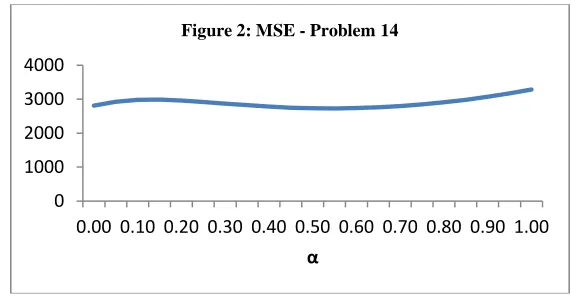
Figure 2 is another case.
The true minimum of MSE occurs at α = 0.54. However, Solver reports the optimal α as 0. Once again, the problem is with the starting value of α = 0. The initial rise in the MSE fools Solver into thinking that the optimal is at α = 0.
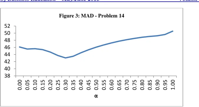
Figure 3 is a final example where the starting value of α results in an incorrect value of optimal α being returned.
0 0.5 1 1.5 2 2.5 3 3.5
0.00 0.10 0.20 0.30 0.40 0.50 0.60 0.70 0.80 0.90 1.00 α
Figure 1: MAD - Problem 4
0 1000 2000 3000 4000
0.00 0.10 0.20 0.30 0.40 0.50 0.60 0.70 0.80 0.90 1.00 α
The optimal value returned is α = 0.06, whereas the true optimal value is α = 0.32. Starting from 0, Solver reports the first minimum it encounters as the true minimum MAD and the corresponding α as the optimal value.
These examples show that Solver is sensitive to the starting value of α. With the default GRG Nonlinear solving method, Solver will return a local minimum if one is encountered within a few iterations of the starting value. This was not at all obvious in earlier versions of Solver. Even in the Excel 2010 version of Solver, we have to read the fine print in the Solver Results pane to understand what is being reported. Despite the message that all constraints and optimality conditions are satisfied, what we are getting is a local optimal solution (see Figure 4).
Figure 4: Solver Results Pane
The obvious way of dealing with the issue of starting value is by picking different starting values. If this had to be done manually, it would be tedious. Fortunately, Solver provides a Multistart option. This is accessed by clicking on the Options button, and then from the GRG Nonlinear tab, checking the Use Multistart box. Now when Solver returns the optimal solution it will report: “Solver converged in probability to a global solution.” In all 21 problems, using the Multistart option with the GRG-Nonlinear engine gave us the correct values of α that minimized MAD/MSE.
38 40 42 44 46 48 50 52
0.00 0.05 0.1
0
0.15 0.20 0.25 0.30 0.35 0.40 0.45 0.50 0.55 0.60 0.65 0.70 0.75 0.80 0.8
5
0.90 0.95 1.00 α
Figure 3: MAD - Problem 14
Solver found a solution. All constraints and optimality conditions are satisfied.
Another option is to use Solver’s Evolutionary engine - one of the three solving methods that Solver now provides in standard Excel. This method is based on genetic algorithms and Solver recommends it for non-smooth functions (expressions that include functions like IF, COUNTIF, MAX, MIN, etc.). There is no guarantee that an optimal solution will be found, but this should not be a difficulty in the simple one or two variable optimization problem we are dealing with here. For each of the textbook-type problems examined in this paper, the Evolutionary engine correctly identified the optimal values of the smoothing constants. However, it does take much longer than GRG-Nonlinear with the Multistart option to report its final solution. This makes it the less desirable approach.
Exponential Smoothing with Trend Adjustment (Holt’s Method)
We solved 11 problems involving exponential smoothing with trend (Holt’s Method) from the same three sources. We created two-dimensional data tables that allowed us to identify the optimal combination of (α, β). Detailed results are presented in Appendix 2.
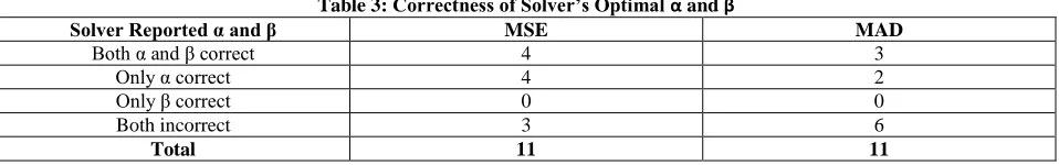
The results were similar to what we saw in the case of simple exponential smoothing. With starting values of both constants set to zero, Solver (Nonlinear Engine without the Multistart option) reported optimal values of α that were correct for 8 of the 11 problems (with an MSE objective) and for only 5 of the 11 problems (with a MAD objective). Similar figures for β were much poorer: 4 out of 11 (MSE objective) and 3 out of 11 (MAD objective). Table 3 summarizes this situation.
Table 3: Correctness of Solver’s Optimal α and β
Solver Reported α and β MSE MAD
Both α and β correct 4 3
Only α correct 4 2
Only β correct 0 0
Both incorrect 3 6
Total 11 11
Overall, Solver’s performance was worse than with simple exponential smoothing and the reason for the poor performance is the same as before – sensitivity to starting values and the tendency to stop the search at a local minimum.
Using Multistart with the Nonlinear Engine allowed Solver to return the correct optimal values of α and β in all cases. This was confirmed using the tabulations of MSE and MAD in the data tables.
Once again, there is a large number of problems with 0 and 1 as optimal values for α and β. For example, when we minimize MSE, 8 of the 11 problems have at least one of α or β at an extreme value (0 or 1). We see similar numbers with MAD.
OPTIMIZING STARTING FORECASTS
Researchers like Bermudez, Segura, & Vercher (2006) have suggested that in addition to the smoothing constants, the starting forecast should also be selected to minimize some error function like MAD or MSE. Textbooks like Chopra & Meindl (2013) have discussed this suggestion in their coverage. We implemented this for each of our 21 simple exponential smoothing textbook problems as well as the 11 exponential smoothing with trend problems. The results for simple exponential smoothing (detailed in Appendix 3) were very similar to the earlier ones, with over 50% of the problems having α = 0 or α = 1 solutions. But the number of problems with optimal α = 0 more than doubled. With two decision variables, Solver slowed down considerably with solution times for some problems in minutes rather than seconds.
regardless of whether MAD or MSE was being minimized. However, when the initial level and trend were also optimized, 9 of the 11 problems had optimal α = 0 (Appendix 4).
DISCUSSION
The results have important implications for the use of Solver in finding the optimal values of smoothing constants in exponential smoothing. As our examples demonstrate, naïve use of Solver to address this problem can lead to results that can be wrong. Solver’s Nonlinear engine only looks for local optima and can be misled by the starting value in problems where the error function is non-convex, discontinuous, or has local minima. It is not possible a priori to determine what kind of function one is dealing with and when Solver will be wrong. Fortunately, Solver itself provides a convenient solution through the Multistart option. Forecasting researchers have been aware of the nonlinearity of the MSE and MAD functions and the possibility of local minima, and recommended the use of multiple starting values (see, for example, Bermudez, Segura, & Vercher (2006)). But textbooks that discuss the optimization approach have ignored these issues. They should revise their treatment to include the Multistart recommendation.
Once we chose the Multistart option, we found no deficiencies in Solver, except that it was slow. We compared Solver’s answers with actual values of MAD and MSE for different values of α and β and were able to confirm that Solver had indeed found the right optimal values. It is likely that the shortcomings of Solver discussed in McCullough & Heiser (2008) have been addressed. However, Microsoft should clearly highlight what Solver means when it claims to have found a solution.
While the Solver approach can be made to work, we believe it is best used when students have already had some exposure to non-linear programming. Concepts like gradients, starting values, local optima, and scaling will then make much more sense. Typical business curricula do not include non-linear programming. The optimization approach using Solver becomes a black-box; students are asked to use some options and ignore others without knowing why.
With business students, a much more transparent approach to finding optimal smoothing constants is to tabulate MAD or MSE for different values of the constants using Excel’s Data Table feature. This way students know exactly what they are doing – creating a table. This is what we did in this paper to get the correct answers to our test problems (to our knowledge, there are no documented issues with the Data Table feature). The obvious drawback is that the approach is limited to two dimensions. We would not be able to find the best value of a third smoothing constant or of the starting forecast. However, Winter’s model is rarely covered in introductory discussions of forecasting and Solver, given its slowness with three or more variables, is not our recommended approach to finding a starting forecast.
Aside from the correctness of Solver’s solutions, our results highlight a more basic issue - the number of problems for which the optimal values of α and β are 0 or 1.
These extreme values of optimal α and β need discussion. A value of α=1 implies that this period’s demand is next month’s forecast (or level estimate) – the so-called naïve forecasting method. A value of α = 0 implies that the demand in a given period is irrelevant to the forecast for the next period: Ft+1 = Ft for all t. In other
words, the initial forecast is the forecast for all subsequent periods. This can happen if the initial forecast is close to the average of the series. If the data has no trend, MSE is minimized if each forecast is close to the average of the data. This is achieved by making minimal changes to the initial forecast; i.e., making α small or even 0. Larger values of α will be necessary if the initial forecast is not comparable with the data. By favoring actual demand larger α will bring future forecasts into line with the data. The same logic holds good with MAD.
The issue of β can also be explained. If β is 0, the initial trend component, T0, is the trend component for
all periods; it is never revised. This might be the case if T0 is a good estimate based, for example, on a linear
regression. If β is 1, trend is estimated as the difference between the two most recent demands.
(6)
and equation (5) as:
(7)
Thus, the actual value of β is irrelevant and the initial trend estimate is the estimate for every period thereafter. When α is 0, both the initial level and trend components are retained for every period and never revised. When we used Solver to optimize L0 and T0, we got optimal α value of 0 for 9 of the 11 problems. Optimization
gave us initial values that modeled the data well enough to never need any revision through the smoothing constants.
Most of the textbook problems we examined had only a few periods of past data – typically 9 periods. It is difficult to see a trend, let alone changes in this trend, with such a small number of periods. It is relatively easy to find initial forecasts that are compatible with the entire data. This is perhaps the reason for the large number of α= 0 solutions when the initial forecast is optimized. However, with a larger number of periods of past data, the likelihood is high that the trend in the data will change making the initial forecast incompatible with at least some portion of the data. This will require smoothing constants that will assign significant weight to both the data and the forecast. Thus, optimal values of α and β that are 0 or 1 should arise less frequently.
While it is a good idea to determine the initial forecast also through optimization along with the smoothing constants, the deterioration in Solver’s solution times makes it impractical in a classroom setting. A better idea is to use an initial forecast that is close to the demand values of the initial periods or to estimate it through a technique such as regression. Regression can also be used to determine starting values for trend.
The extreme values of α and β that result from optimization conflict with the recommendation of most introductory textbooks to keep smoothing constants small, no more than 0.50. The basis for this recommendation, theoretical or empirical, is not clear. Gardner (1985), in his review of exponential smoothing, concludes “… there is no evidence to support such a restricted range of parameters.” He adds, “it is dangerous to guess at values of the smoothing parameters. The parameters should be estimated from the data.”
In any case, it cannot be assumed that the underlying demand generation process will stay the same in the future. It seems prudent to continuously monitor forecasts using MAD, MSE, MAPE, or some other measures of forecast error and use values of α and β that keep these measures within acceptable limits.
In summary, the results of this paper show:
Solver, in its default mode using the Nonlinear Engine, might provide incorrect optimal smoothing constants. This can happen when there is a local optimum near the starting solution.
Solver, with the Multistart option, provides a convenient and reliable way of determining the optimal values of the smoothing constants used in exponential smoothing. Textbooks that present the optimization approach to the smoothing constants should emphasize the Multistart option.
Some background in basic non-linear programming would make students better users of Solver.
Often the optimal values of the smoothing constants are outside the range of values traditionally recommended by business textbooks. For the purposes of selecting smoothing constants to start a set of new forecasts, we believe that the traditional guidelines should be ignored.
These results are true whether we minimize MAD or MSE and whether we assume a starting forecast or determine optimal values of the starting forecast from the data along with the smoothing constants.
In principle, optimization is a good way of determining initial forecasts. However with more decision variables to be optimized, Solver becomes so unpredictable and slow that it is not appropriate for use in the classroom. It is better to find a starting forecast through averaging or regression.
FURTHER RESEARCH
An obvious area for further research is to extend this investigation to forecasting situations involving data sets that are larger than the textbook problems that we used in this paper. This would allow us to confirm the hypothesis that with a larger number of past periods of data, we would see fewer instances where the optimal smoothing constants are 0 or 1.
Further, for the sake of completeness, we should also look at time series with seasonality and the optimization of the smoothing constants in Winter’s model using Solver.
ACKNOWLEDGEMENT
This paper has benefited enormously from the comments of Professors Ram Misra and Mark Berenson both of the Department of Information and Operations Management at the School of Business, Montclair State University. My heartfelt thanks to them.
AUTHOR INFORMATION
Handanhal Ravinder has been an associate professor in the Information and Operations Management department in the School of Business at Montclair State University since Fall 2012. Prior to that, he spent 12 years in the healthcare industry in various market research and business analytics positions. Dr. Ravinder received his Ph.D. from the University of Texas at Austin and taught for many years at the University of New Mexico. His research interests are in operations management, healthcare supply chain, and decision analysis. He has published in Management Science, Decision Analysis, and Journal of Behavioral Decision Making, among others. E-mail: [email protected]
REFERENCES
1. Balakrishnan, N., Render, B., & Stair, R. (2013). Managerial Decision Modeling with Spreadsheets, 3rd Edition, Prentice Hall.
2. Bermudez, J.D., Segura, J.V., & Velcher, E. (2006). Improving Demand Forecasting Accuracy Using Nonlinear Programming Software. Journal of the Operational Research Society, 57, 94-100.
3. Chopra, S. & Meindl, P. (2013). Supply Chain Management: Strategy, Planning, and Operation, 5th Edition, Prentice Hall, Page 195, Chapter 7.
4. Gardner, E.S. (1985). Exponential Smoothing – The State of the Art. Journal of Forecasting, 4, 1-28. 5. Gardner, E.S. (2006). Exponential Smoothing – The State of the Art – Part II, International Journal of
Forecasting, 22, 637-666.
6. Harvey, A.C. (1984). A Unified View of Statistical Forecasting Procedures. Journal of Forecasting, 3, 245-275.
7. Heizer, J. & Render, B. (2011). Operations Management, 10th Edition, Prentice Hall. Page 113, Chapter 4.
8. Jacobs, F. R. & Chase, R.B. (2013). Operations and Supply Chain Management: The Core, 3rd Edition, McGraw-Hill Higher Education, Page 59, Chapter 3.
9. McCullough, B.D. & Heiser, D.A. (2008). On The Accuracy of Statistical Procedures in Microsoft Excel 2007. Computational Statistics and Data Analysis, 52, 4570-4578.
10. Paul, S.K. (2011). Determination of Exponential Smoothing Constant to Minimize Mean Square Error and Mean Absolute Deviation. Global Journal of Research in Engineering, Vol 11, Issue 3, Version 1.0. 11. Schroeder, R., Rungtusanatham, M. J., & Goldstein, S. (2013). Operations Management in the Supply
Chain: Decisions and Cases, 6th Edition, McGraw-Hill Higher Education, Page 261, Chapter 11. 12. Stevenson, W. (2012). Operations Management, 11th Edition, McGraw-Hill Higher Education, Page 87,
Chapter 3.
APPENDIX 1: SOLVER OPTIMAL
α
– SIMPLE EXPONENTIAL SMOOTHINGStarting forecast F1 = Period 1 demand, D1
Reported α: Nonlinear Engine (without Multistart option) Actual α from Data table computation; confirmed with Multistart
Function Type Solver α Actual α Correct? Function Type Solver α Actual α Correct?
1 6 Decreasing 1.00 1.00 Yes Mostly Convex 0.30 0.30 Yes
2 11 Convex 0.31 0.31 Yes Convex 0.13 0.13 Yes
3 5 Convex 0.54 0.54 Yes Convex 0.49 0.49 Yes
4 12 Decreasing 1.00 1.00 Yes Concave 0.00 1.00 No
5 12 Mixed 0.09 1.00 No Mostly Convex 0.77 0.77 Yes
6 11 Decreasing 1.00 1.00 Yes Convex 0.69 0.69 Yes
7 4 Decreasing 1.00 1.00 Yes Decreasing 1.00 1.00 Yes
8 5 Decreasing 1.00 1.00 Yes Decreasing 1.00 1.00 Yes
9 5 Decreasing 1.00 1.00 Yes Decreasing 1.00 1.00 Yes
10 4 Increasing 0.00 0.00 Yes Increasing 0.00 0.00 Yes
11 24 Convex 0.34 0.34 Yes Mostly Convex 0.21 0.21 Yes
12 44 Decreasing 1.00 1.00 Yes Decreasing 1.00 1.00 Yes
13 12 Increasing 0.34 0.34 Yes Increasing 0.30 0.30 Yes
14 10 Mostly Convex 0.00 0.54 No Mostly Convex 0.06 0.32 No
15 12 Mostly Convex 0.00 0.31 No Mostly Convex 0.00 0.58 No
16 16 Convex 0.71 0.71 Yes Convex 0.63 0.63 Yes
17 9 Convex 0.45 0.45 Yes Convex 0.69 0.69 Yes
18 10 Increasing 0.00 0.00 Yes Increasing 0.00 0.00 Yes
19 12 Convex 0.14 0.14 Yes Convex 0.26 0.26 Yes
20 5 Decreasing 1.00 1.00 Yes Decreasing 1.00 1.00 Yes
21 12 Convex 0.43 0.43 Yes Convex 0.41 0.41 Yes
MSE MAD
APPENDIX 2: SOLVER OPTIMAL
α
ANDβ
– EXPONENTIAL SMOOTHING WITH TREND ADJUSTMENT (HOLT’S MODEL)Level estimate L0 = Period 1 demand D1. Trend adjustment T0 = 0. F1 = L0 + T0
Reported α, β: Nonlinear Engine (without Multistart option)
Actual α and β from data table computation; confirmed with Multistart
Reported
Actual Correct? Reported
Actual Correct?
alpha
0.00
0.000
Yes
0.00
0.000
Yes
beta
0.00
0.225
no
0.00
0.612
no
alpha
0.00
0.255
no
0.00
0.274
no
beta
0.00
1.000
no
0.00
1.000
no
alpha
0.00
0.310
no
0.00
0.202
no
beta
0.00
0.166
no
0.00
0.258
no
alpha
0.00
0.70
no
0.00
0.67
no
beta
0.00
0.44
no
0.00
0.45
no
alpha
0.00
0.00
Yes
0.00
0.00
Yes
beta
0.00
0.30
no
0.00
0.00
Yes
alpha
0.00
0.00
Yes
0.00
0.00
Yes
beta
0.00
0.03
no
0.00
0.20
no
alpha
0.55
0.55
Yes
0.45
0.45
Yes
beta
0.08
0.08
Yes
0.00
0.00
Yes
alpha
0.00
0.00
Yes
0.00
0.19
no
beta
0.00
0.05
no
0.00
0.88
no
alpha
0.06
0.06
Yes
0.79
0.05
no
beta
1.00
1.00
Yes
0.00
1.00
no
alpha
0.76
0.76
Yes
1.00
0.76
no
beta
1.00
1.00
Yes
0.51
1.00
no
alpha
0.11
0.11
Yes
0.13
0.13
Yes
beta
1.00
1.00
Yes
1.00
1.00
Yes
9
10
11
6
9
24
44
12
16
9
10
12
5
12
4
5
6
7
8
MSE
MAD
1
2
3
APPENDIX 3: COMPARISON OF OPTIMAL
α
FROM SOLVER – INITIAL FORECAST ASSUMED VERSUS INITIAL FORECAST OPTIMIZEDMSE
MAD
MSE
MAD
1
1.00
0.30
0.00
0.00
2
0.305
0.133
0.00
0.00
3
0.54
0.49
1.00
1.00
4
1.00
1.00
1.00
1.00
5
1.00
0.77
0.93
0.92
6
1.00
0.69
0.92
0.88
7
1.00
1.00
0.00
0.00
8
1.00
1.00
0.74
0.67
9
1.00
1.00
0.81
0.70
10
0.00
0.00
0.00
0.00
11
0.34
0.21
0.27
0.27
12
1.00
1.00
1.00
1.00
13
0.00
0.00
0.00
0.00
14
0.54
0.32
0.56
0.33
15
0.31
0.58
0.36
0.46
16
0.71
0.63
0.71
0.65
17
0.45
0.69
0.00
0.67
18
0.00
0.00
0.00
0.00
19
0.14
0.26
0.00
0.00
20
1.00
1.00
0.82
0.68
21
0.43
0.41
0.00
0.00
Assumed Initial
Forecast
Optimized Initial
Forecast
Problem #
Assumed Initial Forecast:
F
1= D
1Optimized Initial Forecast: Solver
determines F
1in addition to α such
that MAD/MSE is minimized.
With optimized initial forecast, we
see many more cases of optimal α =
0. The initial forecast is good enough
to make further adjustment
APPENDIX 4: EXPONENTIAL SMOOTHING WITH TREND (HOLT’S MODEL) COMPARISON OF OPTIMAL
α
ANDβ
FROM SOLVER – INITIAL L0 AND T0 ASSUMED VERSUS INITIAL L0 AND T0OPTIMIZED