Load Frequency And Voltage Control Of Multi-Area Smart Grid

(1)

Load Frequency And Voltage Control Of

Multi-Area Smart Grid

Krishna Rayalu, K.Saiteja

Abstract: Practical power system is a multi-area system interlinking several areas. These days demand for electrical load is growing tremendously. Conventional grids on their own are not able to meet the load demands which are increasing day by day because as there is a limitation on generation by reserves like coal, water etc. Frequency problems may arise due to this limitation on generation. Load Frequency Controllers which already exist may not possibly solve this frequency problem. This resulted in Smart Grids with renewable generation like wind, solar etc. and Plug in Hybrid Electric Vehicle (PHEV) which can supply the increased load demand from different energy sources. Smart grids are a reality which needs to be backed up by good controllers. In view of practical power system model a four-area interconnected system is considered. Load Frequency Controller (LFC) and Automatic Voltage Regulator (AVR) are the two major parts of power systems which maintain real and reactive power balances under steady state operation. In practical power system scenario these LFC and AVR are interconnected. Hence we consider the interlinking of LFC and AVR for the simulation study of a four area power system. Accordingly in this paper an attempt is made to find the best suited controllers for LFC and AVR of interlinked multi-area system with V2G control of PHEV.

Keywords: Load Frequency Control, Automatic Generation Control, Automatic Voltage Regulator, Smart Grid, Plug in Hybrid Electric Vehicle, Vehicle-to-Grid Control, Battery State-Of- Charge, PID Controller, Active Disturbance Rejection Controller

————————————————————

1. INTRODUCTION

The global energy shortage has directly obstructed the economic, social, developing nations and environments by Green House Gases and by receiving carbon credits. The growing demand for power across the globe is being forecasted and projected to be exponential. Lack of quality with out-of-date network infrastructure, climate change, increasing fuel costs, has resulted in ineffective and progressively unstable electric system. With the growing challenge of electrical power, Quality of service and continuity of supply has been the maximum importance for all major power utility sectors across the world. Smart Grid is predominantly proposed as the major growth in connecting communication and information technologies to enhance grid reliability, and to enable incorporation of various smart grid resources such as renewable energy, electric storage (Battery storage, Vehicle-to-Grid (V2G) storage,… etc.) and electric transportation. Power system may be consisting of single generator or it may have interconnected areas consisting of many generators. The latter is the normal power system. Interconnected System is a big electrical network which is divided into groups known as control areas and each control area corresponds to the portion of the grid owned by a single utility. Lines joining different control areas are known as tie-lines. With the expansion of non-conventional energy coming from resources as wind and sun, there is huge increase in the number of distributed generations. These non-conventional energy sources are of random nature, specifically wind energy, the energy storage systems of decent number needed greatly to make such resources dependable. The power network assembly turns out to be more complex with the connection of energy storage system and distributed generation to the grid.

The power system which is stressed becomes more difficult to control. The non-conventional generation and load are of varying nature. The real and reactive powers demanded by the different loads are to be delivered by an electric power system. The delivered power must be continuous and also come across certain minimum necessities concerning the supply quality such as, invariable rated voltage, invariable rated frequency and a high reliability. A slight change in the mechanical input of the generator will affect the system frequency while changes in the generator excitation system will disturb the system voltage. Thus it is appropriate to divide the power system control into two separate sections one is the megawatt frequency control and the other is the megaVAr voltage control. The active power control of the generator output, in response to the variations in the system frequency to maintain planned system frequency and tie-line power transfer is named as Load Frequency Control. Thus Load Frequency Control (LFC) has gained importance in an interconnected system. The system frequency maintenance and the active power control are done by LFC control loop. The reactive power balance control of the system is treated separately and excitation control of the generator units concerns about to maintain the scheduled voltage of the system named as Voltage Control. The reactive power and the magnitude of voltage are controlled by the Automatic Voltage Regulator (AVR) loop. The generator reactive power is organized by the control of generator excitation using AVR. The objective of AVR is to maintain the terminal voltage of the generator constant at nominal value during normal operating conditions at different load levels. The excitation system of AVR control loop employs terminal voltage error to change the field voltage to control the generator terminal voltage. To reduce the global climate change and to enhance the energy security, new technologies that reduce the CO2

emissions have been investigated for some years. The interest in battery electric vehicles (BEVs) and plug-in hybrid electric vehicles (PHEVs) has increased due to their ability to reduce the CO2 pollution, low-cost charging, and

reduced petroleum usages. The dynamic response of multiple PHEVs having battery storage is fast and is expected to compensate unbalance in the real power of the system when there is inadequate LFC capacity. The _____________________________

 M.S. Krishna Rayalu, Electrical & Electronics Engineering Dept., V R Siddhartha Engineering College, Vijayawada, India 520007 [email protected]

(2)

875 dynamic response of PHEV is quicker than the dynamic

response of turbine and governor of the thermal generator. Hence PHEV is responsible for damping the peak value of frequency oscillation quickly. Consequently the elimination of the steady state error of frequency fluctuation is carried out by the turbine and governor of thermal generator. The benefits of using PHEV for regulation will vary based on the type and the location of the PHEV. Compared with traditional hybrid electric vehicles (HEVs), BEVs/PHEVs have an enlarged battery pack and an intelligent converter. Using a plug, BEVs/PHEVs can charge the battery using electricity from an electric power grid, which is called as ―grid-to-vehicle‖ (G2V) operation. Similarly discharge of these vehicles to an electric power grid, during the parking hours, is referred to as ―vehicle-to-grid‖ (V2G) operation. The V2G control, based on the average battery State Of Charge (SOC) deviation control, is applied to compensate the LFC capacity in the power system. [7] concentrates on the autonomous distributed V2G control considering the charging request and battery condition for reducing the fluctuations of frequency and tie-line power flow in the two-area interconnected power system. The battery SOC is controlled by the SOC balance method. The parameter values in the power system model vary depending on the system. The power flow conditions of the system also change frequently. Main aim of the control technique is to generate and deliver power in an interconnected system economically and reliably while maintaining the voltage and frequency within prescribed tolerance limits. Hence dealing with the uncertainties of the plant dynamics to choose a controller for LFC and AVR problems is an essential factor. LFC has to be unaffected by unknown external disturbances and internal disturbance such as system model and parameter. PID controller is the most established controller in industry. It is activated based on error and easy to implement. Both transient and steady state performances will be improved by using PID controller. Now ADRC, a robust controller, is being used to resolve problems like transient and steady state performances improvement. Active Disturbance Rejection Controller (ADRC) is a combination of an extended state observer (ESO) and a feedback controller. ESO is a dynamical system with n+1states. ESO is used to observe the n states of the system and the generalized disturbance. The extended state in ESO is used to estimate the total action of the uncertain models and the system disturbances and then is applied to compensate the disturbances. A state feedback control loop tracks error between the real output and a reference signal for the plant. ADRC has been applied in many fields such as aviation, aerospace, electric power system and chemical industries because of its perfect control properties such as fast response of the system, small overshoot, wide adaptation and small undershoot. The objective of this paper is to maintain the frequency and voltage within acceptable limits under internal and external disturbance or both by having the best suited controllers for interlinked LFC and AVR of the considered four-area smart grid power system. Simulation studies are carried out for this system with PID and ADRC controllers to select the best controller.

2. SYSTEM MODELING

A linear model of Power System is developed on the lines of [1]. Automatic Generation Control (AGC) includes primary and secondary control loops with secondary loop controlled by ADRC/PID controllers so that both transient and steady state performances are improved to zero steady state error resulting in rated frequency. Here we employ Tie-line Bias Control (TBC) to keep frequency at nominal value, maintain tie-line flow at scheduled value and each area has to absorb its own load changes. Also TBC makes Area Control Error (ACE) = 0.

∑

Ki – Area bias factor

Area bias Ki determines the amount of interaction during a disturbance in the neighboring areas. For satisfactory performance, Ki = Bi, frequency bias factors. For a two-area

system

ACE1 = ΔP12 + B1Δω1

ACE2 = ΔP21 + B2Δω2

Where ΔP12 and ΔP21 – changes in scheduled

interchanges.

2.1 AGC Including Excitation System

The study of coupling effect extends the linearized AGC system to include excitation system. The small change in real power is the product of synchronizing power coefficient Ps and the change in power angle Δδ. If the small effect of

voltage upon real power is included, then the following linearized equation is obtained:

ΔPe=Ps Δδ+k2E’

where k2 is the change in electrical power for a small

change in the stator emf E’. Also including the small effect of rotor angle upon the generator terminal voltage

ΔVt= k5 Δδ+ k6E’

where k5 is the change in terminal voltage for a small

change in rotor angle at constant E’, k6 is the change in

terminal voltage for a small change in E’ at constant rotor angle. Finally modifying the generator field transfer function to include the effect of rotor angle, the stator emf E’ is expressed as

E’ =

For a stable system Ps, k2, k4 and k6 are positive, but k5 may

be negative. Typical values of the coupling constants are k2=0.2, k4=1.4, k5=-0.1 and the voltage coefficient k6 is 0.5.

(3)

Fig.1 Linear model of the two-area smart interconnected power system

Fig.2 Four-area interconnected power system

2.2 Simulink Models of Considered Four Area System

Fig. 2a Simulink diagram of four-area system LFC with interlinking of AVR

Fig. 2b Subsystem model of V2G control of PHEV

Fig. 2c Simulink diagram of AVR subsystem for area 1

The Simulink diagram of considered four area system with interlinking AVR with LFC control is given in the Fig. 2a. The V2G control model which is given in the subsystem is shown in Fig. 2b. The AVR subsystem model considered four areas is shown in Fig.2c. Here the controllers used are either PID or ADRC based upon the case.

3. V2G POWER CONTROL

[7]

Frequency fluctuation detected from the home outlet is used to observe the unbalance between the supply and load demand of the power grid. Hence with the help of droop characteristics i.e. V2G power against the frequency fluctuation (∆f) there is control of V2G power (PV2G). The

characteristics between V2G power against the frequency fluctuation shown in Fig. 3

Fig. 3 V2G Power Control

Based on the characteristics between V2G power against the frequency fluctuation the V2G power output equations are given as below

{

(3.1)

where KV2G is gain of V2G. By considering the tradeoff

between the outcome of V2G and the variation of range in battery SOC the gain of V2G that is KV2G is tuned. Pmax is

the maximum power of V2G defined by the home outlet of 200V/25A.

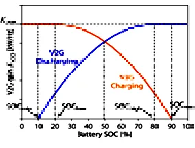
3.1 State Of Charge (SOC) Deviation Control

(4)

877 implemented in order to avoid overcharge (over discharge).

In the period of long lasting V2G cycles, the SOC is suggested to be either completely full or empty since mean value of the frequency variation is not zero all the time and due to this there is a chance of battery failure. Taking all these features into account, a balance control is installed as the following equation on the basis that the estimation of SOC is precise which can be realized as below:

{ (

) } (3.2) where Kmax is utmost gain of V2G. SOCmin, SOClow, SOChigh,

SOCmax and n are the minimum SOC of battery, low SOC of

battery, high SOC of battery, maximum SOC of battery and design parameter correspondingly.

Fig. 4 SOC Balance Control

From the SOC balance control shown in Fig. 4, the SOC of battery can be controlled. Based on (3.1) and (3.2), PV2G

can be organized by tuning the gain of V2G (KV2G) against

the frequency variations. KV2G can be adjusted by the SOC

deviation control within the specified SOC range. Here, the initial SOC and target SOC in area 1, 3 are set at 20% and 90% respectively. Also, in area 2, 4 the initial SOC and target SOC are set at 50% and 50%, respectively.

4. CONTROLLERS

PID and ADRC controllers are employed as secondary controllers for the Load Frequency and Voltage Control problem.

4.1 PID controller

The majority of control systems in the world operate on the traditional Proportional-Integral-Derivative (PID) controller. The qualities of PID controller like having simple structure, easy understanding about functionality and applicability which makes the use of PID controller easy and hence the 95 percent applications of control process in industries make use of PID controller. It is activated based on error and easy to implement. PID controller is used for a wide range of applications like drive motors, automotives, control of planes, etc. Steady and consistent performance is provided for the majority of the systems if the tuning of the PID controller proper. If PID controller is tuned properly it provides robust and reliable performance for most of system. There are numerous tuning methods are available in those Ziegler-Nichols (ZN) technique is very influential. Both transient and steady state performances will be improved by using PID controller. The effect of proportional parameter (KP), integral parameter (KI), derivative

parameter (KD) of the PID controller on the closed loop step

response is as mentioned in the Table 1

Table 1: Effect of PID parameters

Proper selection KP, KI and KD is the tuning of PID

controller. There are numerous tuning methods are available for tuning of PID controller. In this paper MATLAB tuning technique is used for tuning PID controller.

4.1.1 MATLAB Tuning Technique [10]

A transfer function of the PID controller in continuous s-domain is described as follows

)

where is proportional gain, is the integration coefficient and is the derivative coefficient. is the integral action time and is derivative action time. In this controller has three different adjustments ( ) which interact with each other. A methodology for tuning PID controller is given below using Simulink.

Step 1: First we set the gain parameter KP with KD and KI

values set to zero. KP value is selected by using trial and

error method which results a stable oscillatory performance. High KP value gives in decrease of rise time with some

steady state error but highly oscillatory in performance. For single input system we generally employ the high KP value

.In multi input system high KP value it is observed that to

difficult to damp out the oscillations. Hence in multi input select a KP value near to critical damping.

Step 2: Now by using derivative control we can reduce the oscillations which are present in step 1 by providing proper damping which results in reduced settling time and overshoot. By varying KD with KP found in step1 this can be

achieved. Now we have fixed KP and KD Still KI=0.

Step 3: From step 1 and step 2 we have taken care about transient performance. Now we concentrate on steady state performance. If still steady state error exists in system response we have to reduce it to zero by varying the KI with

KP and KD fixed in step 2.Then select the KI value which

results in zero steady state error in minimum time. By this complete the tuning of a PID controller. In some cases PI/PD controller is enough. In that case step 2/step 3 may not be required.

The tuned values of PID controller for the simulation study carried out are given in the Tables 4 and 5.

4.2 ADRC Controller [11-13]

Plant which is of universal form with finite zeros represented by a transfer function of minimum phase is given as below:

, (4.1)

(5)

are the the transfer function coefficients. After performing the longhand division of equation (4.1), the plant is remodeled as given below:

sn-m Y(s)= b0U(s) + D(s) (4.2)

where b0 = bm+1/an+1. D(s) includes both internal and

external disturbances. After remodeling of the considered nth-order system, it has two principal parameters namely plant order (= n-m) and the high frequency gain b0 which

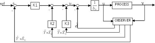
are important parameters for the ADRC design. An Extended State Observer (ESO) is used to nullify the effect of generalized disturbance d(t) by treating the disturbance d(t) as an additional state. Here we employ Bandwidth Parameterization technique by placing poles of observer /controller at single location. The heart of ADRC is ESO. In order ESO to work appropriately, observer dynamics must be quick. The required observer gains are calculated for the location of common pole. is observer bandwidth. In order to locate all the eigenvalues of the ESO at according to Bandwidth Parameterization, the vector element values are selected as

( )

To make the tuning process simple, all the controller closed-loop poles are set to , bandwidth of the

controller. Accordingly the controller gains are selected as (₎

As bandwidth of the controller ωc increases, the output

speed tracking of system controlled with ADRC will increase. In other words the error tracking, overshoot of the output and output settling time will be reduced. Generally, ωc varies from 3~10. Control loop structure of a third order

process with ADRC is given in Fig.5

Fig. 5 Control loop structure of a third order process with ADRC

4.2.1 Design of ADRC gains for LFC ADRC for LFC of area 1:

The transfer function of primary loop of area 1 is

Here n=3, m=0, n-m=3, = 1, =1; b0 = / =1

ADRC for LFC of area 2:

Here n=3, m=0, n-m=3, = 1, =1.44; b0 = / = 0.6944

Here n=3, m=0, n-m=3, = 1, =2.52; b0 = / = 0.3968

Here n=3, m=0, n-m=3, = 1, =1.44; b0 = / = 0.6944

Observer and Controller gains of ADRC for LFC in areas 1, 2 and 4:

The ESO is derived for observer bandwidth 𝜔𝑜 = 20rad/s. Next controller gains are computed for controller bandwidth 𝜔𝑐 = 10rad/s, as

Observer Gains: L1=80; L2=2400; L3=32000;

L4=160000.

Controller Gains: 𝑘1 = 1000; 𝑘2 = 300; 𝑘3 = 30.

Observer and controller gains of ADRC for LFC in area 3: The ESO is derived for observer bandwidth 𝜔𝑜 = 15rad/s. Next controller gains are computed for controller bandwidth 𝜔𝑐 = 10rad/s, as

Observer Gains: L1=60; L2=1350; L3=13500; L4=50625.

4.2.2 Design of ADRC gains for AVR ADRC for AVR of all four areas:

The transfer function of primary loop of areas 1,2,3,4 is

Here n=4, m=1, n-m=3, = 300, =1 Hence b0 = / =300

Observer and controller gains of ADRC for AVR in areas 1,2,3,4:

The ESO is derived for observer bandwidth 𝜔𝑜 = 50rad/s. Controller gains are computed for controller bandwidth 𝜔𝑐 = 10rad/s. The resulting gains are

Observer Gains: L1=200; L2=15000; L3=500000;

L4=6250000.

5. Simulation Studies

5.1 PID controller in both LFC and AVR and ADRC controller in both LFC and AVR for all the interconnected four areas

(6)

879

Fig. 6 Frequency Deviations in Area 1

Fig. 10 Tie-line power Deviations in Area 1

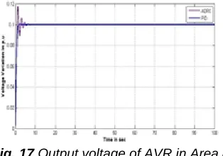
Fig. 14 Output voltage of AVR in Area 1

(7)

5.2 Simulation study with ADRC controller for LFC and PID controller for AVR

Based on the observations of 5.1, the considered four-area system is simulated and analyzed using ADRC controller in LFC and PID controller for AVR. The results are shown in Figs 18-29. From these figures we observe that LFC performance is better than the performance reported in 5.1, whereas AVR performance is same as in 5.1 with PID controller. This is because an improved AVR performance with PID controller resulted in improved LFC performance with ADRC. Hence AVR with PID controller and LFC with ADRC controller give the best performance.

Fig. 18 Frequency Deviation in Area 1

(8)

881

Fig. 26 Tie-line power deviation in Area 1

Table 3: LFC Data for four-areas

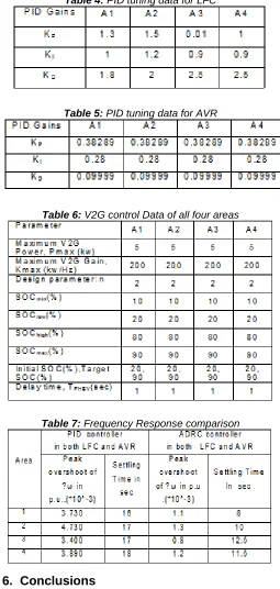
Table 4: PID tuning data for LFC

Table 5: PID tuning data for AVR

Table 6: V2G control Data of all four areas

Table 7: Frequency Response comparison

6. Conclusions

(9)

for AVR are the best with good transient and steady state responses. Accordingly ADRC controllers are used for LFC and PID controllers are used for the AVR for the four-area system considered for best performance in section 5.2. Based on these observations of section 5.2, ADRC is recommended for LFC and PID controller is recommended for AVR for better performance when LFC and AVR are interlinked.

7. FUTURE SCOPE

The internal and external uncertainties assessment and their mitigation in real time can be done by ADRC. For structural uncertainties that commonly exist in power systems, ADRC acts as robust controller against them. ADRC precise model is very robust against the parametric uncertainties of the plant and external disturbances. ADRC also has advantages like perfect control properties such as fast response of the system, small overshoot, wide adaptation and small undershoot. However ADRC controller applications are not thoroughly investigated. Hence more investigations need to be carried out in order to exploit the applications of ADRC to its potential. PID controller is the most widely used controller in industry. Hence similar studies can be carried out for different smart grids for selecting better controller.

ACKNOWLEDGEMENTS

The authors greatly acknowledge Siddhartha Academy of General and Technical Education, Vijayawada for providing the facilities to carry out this research.

REFERENCES

[1]. Hadi Saadat, Power System Analysis, Tata McGraw-Hill, New Delhi, 2007

[2]. Kundur P. Power System Stability And Control. 5th reprint. Tata McGraw Hill; New Delhi: 2008. [3]. Kothari DP, Nagrath IJ. Modern Power System

Analysis. 4/e New Delhi: Tata McGraw Hill; 2011. [4]. Katsuhiko Ogata, Modern Control Engineering, 5/e

PHI, New Delhi, 2010.

[5]. Y. Ota et al., ―Effect of autonomous distributed vehicle-to-grid (V2G) on power system frequency control,‖ in Proc. Int. Conf. Ind. Inf. Syst.(ICIIS), pp. 481–485.

[6]. J. R. Pillai and B. Bak-Jensen, ―Integration of vehicle-to-grid in the Western Danish power system,‖ IEEE Trans. Sustainable Energy, vol.2, no. 1, pp. 12–19, Jan. 2011.

[7]. Sitthidet Vachirasricirikul and Issarachai Nigamroo ―Robust LFC in a Smart Grid with Wind Power Penetration by Coordinated V2G Control and Frequency Controller‖, IEEE Trans. Smart Grid, vol. 5, no. 1, pp.371–380, Jan 2014

[8]. Y. Ota, H. Taniguchi, T. Nakajima, K. M. Liyanage, J. Baba, and A.Yokoyama, ―Autonomous distributed V2G (vehicle-to-grid) satisfying scheduled charging,‖ IEEE Trans. Smart Grid, vol. 3, no. 1, pp.559–564, Mar. 2012

[9]. Zheng Qing and GAO Zhiqiang, ―On Practical Applications of Active Disturbance Rejection Control‖, Proceedings of the 29th

Chinese Control Conference July 29-31, 2010, Beijing, China.

[10]. M.Nagendra and M.S.Krishnarayalu. ―PID Controller Tuning using Simulink for Multi Area Power Systems‖, IJERT, ISSN: 2278-0181, Vol. 1, Issue 7, September - 2012

[11]. Krishnarayalu M.S. and K. Nagarjuna ―AVR with ADRC ―, International Electrical Engineering Journal (IEEJ) Vol. 5 (2014) No.8, pp. 1513-1518, ISSN 2078-2365

[12]. Krishnarayalu M.S. and K. Nagarjuna “ADRC for Two-Area LFC‖ , IJERT, ISSN: 2278-0181,Vol. 3 Issue 11, November – 2014, pp 141-146