317
Panel Data Model For Tourism Demand
Kadek Jemmy Waciko, Ismail, B
Abstract -This study explained the construction of panel data models, compared the estimation performance of the Fixed Effects model and the Random Effects model. Our novelty model focuses on the 10 best travel destinations according to Tripadvisor award 2018. The most appropriate model is the Fixed Effect model with Individual Effect. The positive effect on Gross Domestic Product (GDP) partially arising from Number of International tourist arrivals, International Tourism Receipts, and International Tourism Expenditures and the negative effect on GDP partially arising from Total Employment in the tourism sector. The International Tourist Arrivals, International Tourism Receipts, International Tourism Expenditures, and Total Employment in the tourism sectors have simultaneous significant influence on GDP and adjusted together can explain changes in GDP by 95.054% from France, UK, Italy, Indonesia, Greece, Spain, Czech Rep., Morocco, Turkey, and the USA while the remaining 4.946% is explained by other variables outside the model.
Keywords: Fixed Effects model, Random Effects model
——————————
——————————
1.
INTRODUCTION
The phenomenal growth of both the world-wide tourism industry and academic interest in tourism over the last forty years has generated great interest in tourism demand modeling and forecasting from both the business and academic sectors. Lim [12] noted that, although time series data are widely utilized in estimating tourism demand, few studies use cross-section or panel data. As an overview, we can see in [14] used panel data to develop a model of international tourism spending using both economic and social variables for a total of 138 countries over 7 years.The use of the data panel approach to identify the recent effects of demographic change in Japanese people’s travel Propensity is also used in [15]. On the other hand, [11] estimated short-run and long-short-run elasticities for tourists visiting the Island of Tenerife. In addition, [13] identified factors affecting tourist arrivals to Africa. Garin-Munoz [5] and Garin-Munoz & Montero-Martin [6] modeled international tourism demand for the Canary Islands and the Balearic Islands, respectively. Some other interesting research that uses data panels in tourism demand we can see in [16] examined whether climate change has impacted regional tourism in the UK. Brida & Risso [2] studied the German demand for tourism in South Tyrol using dynamic panel data. The impact of Avian Flu on international tourist arrivals to Asian, European and African countries estimated in [10] and a panel data model of international tourism demand for Malaysia developed in [8]. Panel data are most useful when we suspect that the outcome variable depends on explanatory variables that are not observable but correlated with the observed explanatory variables. Parameter estimation in regression analysis with cross-section data carried out with OLS estimation. This method will give the results of the estimationwhich is the Best Linear Unbiased Estimator (BLUE) if all of the Gauss Markov assumptions are met including non-autocorrelation. When we are dealing with panel data, this last condition is certainly difficult to fulfill so that parameter estimation is no longer for BLUE. If panel data is analyzed by approaching time series
models, then there is information on the variety of unit cross-sections that are ignored in modeling. One of the advantages of panel data analysis is considering thevariety that occurs in unit cross-sections. The purpose of this study:
1) To explain proportionally the construction of panel data models using the application in tourism demand.
2) To compare between the Fixed Effects Model and the Random Effects Model approaches to found the appropriate model.
3) To estimates parameter the appropriate model using diagnostic test criteria.
2.
METHODOLOGY
2.1 Pooled Regression Model
The equation for the Pooled Regression model :
t i t i t i t
i x
y . ', , ,
(1) Where:
t i
y . is the dependent variable where i represents countries
(the cross-section dimension) and t represents time (the
time-series dimension); xi',t is vector of K- independent variables
from country-i and observed in time-t; i,t is the error
term, The error term is identical and independently distributed
or iid (0,2) for all i and t.
2.2 Fixed Effects Model
The equation for the Fixed Effects model:
(2) , ,
' ,
.t it it i t it
i x c d
y
Where cidenotes the unobservable individual effects; dt
denotes the unobservable time effects. If the model contains
i
c and dt, is called a two-way fixed effects model, if the
model contains dt 0 or ci 0 called a one-way fixed
effects model.
2.3 Random Effects Model
Random effects models are generally written as follows :
(3)
, , '
,
.t it it it
i x w
y
Where, _____________________________
Kadek Jemmy Waciko. Research Scholar, Department of Statistics, Mangalore University, Mangalagangothri-574199, Karnataka, India. Email: [email protected]
318 (4) t i, , c d wit i t
If the model contains ci and dt, is called a two-way random
effects model, if model contains dt 0 or ci 0 called a
one-way random effects model.
2.4. Estimation Methods
2.4.1 Generalized Least Squares
Suppose, Wi
wi1,wi2,...,wiT
' In view of this form of wit ,we have what is often called an “error components model” then, for this model,
, . , 2 2 2 2 s t w w E w E u is it u it For the T observations for unit i, let E
wiwi
. Then(5) 2 2 2 2 2 2 2 2 2 2 2 2 2 2 2 2 2 T T u T u u u u u u u u u u u u i i I
Where I is a T x1 column vector of 1s. Since observations I and j are independent, the disturbance covariance matrix for the full nT observations is
(6) 0 0 0 0 0 0 0 0 0 n I
V
This matrix has a particularly simple structure. For
generalized least squares, we require 2 1 2 1 I V
therefore, we need only find 2 1
, which is
ii
T I 1 2 1 Where 2 2 1 u T
the transformations ofyi and
i
X for GLS is therefore
. . 2 . 1 2 1 1 i iT i i i i i y y y y y y y (7)
and likewise for the rows of Xi. For the data set as a whole,
generalized least squares is computed by the regression on these partial deviations of yit on the same transformation of
it
x . Note the similarity of this procedure to the computation in
the LSDV model, which has 1. It can be shown that the GLS estimator is, as the OLS estimator, a matrix weighted average of the within and between units estimators:
b W W W b F I b
Fˆ ( ˆ )
ˆ
(8) We can see the detail explained in [7].
2.4.2. General Feasible Generalized Least Squares Models The estimated error covariance matrix is
ˆ ˆ n I
V , with
n i T it it n u u 1 ˆ ˆˆ (9)
the error or mismatched covariance structure inside every group (if Effect= “Individual”) of observations to be fully unrestricted may be affected by this framework. We can see the detail explained in [4].
2.5 Model Analysis
2.5.1 Hausman’s Test
We can run a Hausman test to decide between fixed or random effects where the null hypothesis is that the preferred model is random effects vs. the alternative the fixed effects. It basically tests whether the unique errors (ui) are correlated with the regression, the null hypothesis is they are not. Hausman (1978) in Greene [9] developed a test based on the idea that under the hypothesis of no correlation, The other essential ingredient for the test is the covariance matrix of the
difference vector,
b ˆ
:
bˆ
Var b Var
ˆ Cov
b,ˆ Cov
b,ˆVar (10)
Hausman’s essential result is that the covariance of an efficient estimator with its difference from an inefficient estimator is zero, which implies
(b ˆ),ˆ
Cov
b,ˆ Var
ˆ 0Cov or that
b,ˆ Var
ˆCov
Inserting this result in (10) produces the required covariance matrix for the test,
b ˆ
Var
b Var
ˆ Var (11) The chi-squared test is based on the Wald criterion:
ˆ ˆ 1 ˆ
K b b
W (12)
For ˆ , we use the estimated covariance matrices of the slope estimator, in the LSDV model and the estimated covariance matrix in the random effect model, excluding the constant term. Under the null hypothesis, W is asymptotically distributed as chi-squared with K degrees of freedom .
2.5.2 Breusch and Pagan’s Test
This test aims to see whether there are individual/time (or both) effects in the data panel, namely by testing the hypothesis in the form
0 , 0 :
0 ci dt
H , or there is no two-way effects
0 : 0 ci
H , or there is no individual effects
0 : 0 dt
H , or there is no time effects
We look at a Lagrange Multiplier test developed by Breusch and Pagan (1980), the test statistics are given by
319 2.5.3.Breusch-Godfrey/Wooldridge Test
Under the null of no serial correlation in the errors, the residual of a model must be negatively serially correlated, with
) 1 /( 1 ) ˆ ˆ
( , T
cor it for each t,s. Wooldridge suggests
basing a test for this null hypothesis on a pooled regression of FE residuals on themselves, lagged one period:
t i t i t
i, ˆ, 1 ,
ˆ
(14) Rejecting the restriction 1/(T 1). Makes us conclude against the original null of no serial correlation.
2.5.4. Pesaran CD Test
Pesaran (2004) recommended a simple test of error cross-section dependence (CD) that is applicable to variety of panel models, including stationary and unit root dynamic heterogeneous panels with small T and Large N. The proposed test is based on an average of pairwise correlation coefficients of OLS residuals from the individual regressions in the panel rather than their squares as in the Breusch-Pagan LM test:
(15) ˆ ) 1 ( 2 1 1 1 N i N i j ij ij T N N T CD Where
1/21 2 2 / 1 1 2 1 ˆ T t it T t it T t jt it ij e e e e
,ˆij is the
product-moment correlation coefficient of a model’s residuals; eit denoting the OLS residuals based on T observations for each i=1,….,N. In the case of an unbalanced panel only pairwise complete observations are considered, and
) , min( i j
ij T T
T with Ti being the number of observations
for individual I; else, if the panel is balanced, Tij T for each
j
i, . Under the null hypothesis of cross-section in dependence, CD~N(0,1).
2.5.5. Robust Covariance Matrix Estimation.
Wald-type tests is used for Robust estimators of the covariance matrix of coefficients, consistent vs. serial correlation is generally results in the context of panel data version, see in [7]. Basically, all types assume there is no correlation between errors of different groups while allowing for heteroskedasticity. All types assume no correlation between errors of different groups while allowing for heteroskedasticity but no serial correlation, i.e.
(16) 0 0 0 0 2 2 2 2 1 iT i i i
While “White2” is “White1” limited to a common variance
inside every group, estimated as
T t it i T u 1 2 2 ˆ
so that
2 i T i I
, lets a totally general structure w.r.t heteroskedasticity and serial correlation
) 17 ( , , , 0 , , 2 1 1 1 2 2 1 2 1 2 1 iT iT iT i iT iT iT i iT i i i i i
The latter is, as already observed, consistent w.r.t timewise correlation of the errors, but on the converse, unlike the White 1 and 2 methods,it relies on large n asymptotics with small T.
3.
AN EMPIRICAL STUDY
3.1. The Novelty of the Model
TripAdvisor, the leading travel review site, has ranked the world’s best travel destinations of 2018. The site’s Travelers’ Choice Awards for destinations recognized travelers’ favorite destinations around the world. According to TripAdvisor award 2018, the 10 Best Travel Destinations in 2018: 1). Paris, France; 2). London, United Kingdom; 3) Rome, Italy; 4). Bali, Indonesia; 5). Crete, Greece; 6). Barcelona, Spain; 7). Prague, Czech Republic; 8). Marrakech, Morocco; 9). Istanbul, Turkey; 10). New York City, USA. This is a novelty model in tourism demand focus on the 10 best travel
destinations of 2018 and data are compiled from
https://data.worldbank.org, for the period 1995 to 2017.
This study examines the relationship between Gross
Domestic Product (GDP) is related the Number of International Tourist Arrivals, International Tourism Receipts, International Tourism Expenditures, Tax Revenue in the tourism sector, and Total Employment in the Tourism sector. After transformation original data used natural log, the panel model represent as:
t i t i
it X X X X X c d
Y 1log 1 2log 2 3log 3 4log 4 5log 5 , log
Where the variable definitions for country i are:
it
Y = Gross Domestic Product for country i (US$);
1
X =Number of International Tourist Arrivals for country i
(number of person); 2
X = International Tourism Receipts for country I (US$);
3
X = International Tourism Expenditures for country i
( US$);
4
X = Tax Revenue in tourism sector for country i (%);
5
X = Total Employment in tourism sector for country i(%); ; ...X X for coeficient Slope , , ,
, 2 3 4 5 1 5
1
i
c the unobservab le individual effects;
t
d = the unobservable time effects; term e disturbanc usual the it
i = 1,2,…….10 (the 10 Best Travel Destinations in 2018); t =1,2,……230 (from 1995- 2017).
R-studio software is used for panel model analysis. To describe the calculation of the panel model where the panel models will be estimated is presented as follows:
Model I :
t i t d i c X X X X X t i Y , 5 log 5 4 log 4 3 log 3 2 log 2 1 log 1 ,
log
320 t
i t d i c X X
X X
t i
Y ,
4 log 4 3 log 3 2 log 2 1 log 1 ,
log
Model III:
t i t d i c X X
X X
t i
Y ,
5 log 5 4 log 4 2 log 2 1 log 1 ,
log
3.2. Analysis Model
3.2.1. Hausmann Test
In this study, we used the transformation model with natural log, and then for the analysis model, first of all, we consider to used Hausmann Test for data.
Table 1. Hausmann Test
Model Statistics Test p-value Conclusion Model I 6.2911 0.2789 Fixed Effects Model II 12.958 0.01148 Random Effects Model III 4.0757 0.3959 Fixed Effects Ho: Fixed Effects model is used for Panel Model. H1: Random Effects model is used for Panel Model.
The Hausman test helps us to decide between the fixed effects and Random effects or to select the model will be used for analysis. In this case, if the p-value >0.05 then use Fixed effects, if not use random effects.
3.2.2. Breusch-Pagan Test
Summary result of Breusch-Pagan test is given in the following table 2.
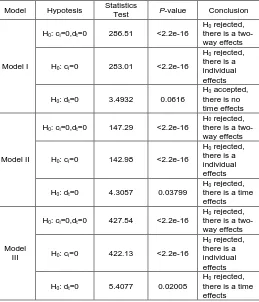
Table 2. Breusch-Pagan test
Model Hypotesis Statistics
Test P-value Conclusion
Model I
H0: ci=0,dt=0 286.51 <2.2e-16
H0 rejected, there is a two-way effects H0: ci=0 283.01 <2.2e-16
H0 rejected, there is a individual effects H0: dt=0 3.4932 0.0616
H0 accepted, there is no time effects
Model II
H0: ci=0,dt=0 147.29 <2.2e-16
H0 rejected, there is a two-way effects H0: ci=0 142.98 <2.2e-16
H0 rejected, there is a individual effects H0: dt=0 4.3057 0.03799
H0 rejected, there is a time effects
Model III
H0: ci=0,dt=0 427.54 <2.2e-16
H0 rejected, there is a two-way effects H0: ci=0 422.13 <2.2e-16
H0 rejected, there is a individual effects H0: dt=0 5.4077 0.02005
H0 rejected, there is a time effects From table 2, it can be concluded that the models are presented as follows:
1) Model I (Fixed Effects model with individual effects),
2) Model II (Random Effects model with two-way effects), 3) Model III (Fixed Effects model with two-way effects)
3.3. Model Estimation
To estimate the Fixed Effects model and Random Effects model we used The Generalized Least Squares (GLS) and Feasible Generalized Least Squares (FGLS). Model I, model II and model II are reduced to the new models, namely:
1) Model A (Fixed-Effects Model with Individual Effects).
t i i c X X
X X
t i
Y, 1log 1 2log 2 3log 3 5log 5 , log
2) Model B (Random-Effects Model with two-way effects).
t i t d i c X X
t i
Y ,
3 log 3 1 log 1 0 ,
log
3) Model C (Fixed-Effects Model with two-way Effects).
t i t d i c X X
X t
i
Y, 1log 1 2 log 2 5 log 5 ,
log
3.4. Diagnostic Tests
3.4.1. Testing for Serial Correlation
In this study, we used the Breusch-Godfrey/Wooldridge test for serial correlation in panel model where
H0: There is no serial correlation.
H1 : There is serial correlation.
Table 3.
Breusch-Godfrey/Wooldridge Test
Model Panel
Statistics Test
p-Value Conclusion
Model A 0.51537 0.7728
There is no serial correlation
Model B 1.7725 0.4122
There is no serial correlation
Model C 0.7699 0.6805
There is no serial correlation
Interpretation for model A: “p-value < 0.7728, accepted H0, there is no serial correlation; Interpretation for model B: “p-value < 0.4122, accepted H0, there is no serial correlation;
and Interpretation for model C: “p-value < 0.6805, accepted
0
H , there is no serial correlation.
3.4.2.Testing for cross-sectional dependence
The null hypothesis in Pasaran CD tests of independence is that residuals across entities are not correlated or connected. The residuals are tested by Pasaran CD (cross-sectional dependence) and it will be correlated across entities*. Cross-sectional dependence can lead to bias in tests results (also called contemporaneous correlation)
Ho: There is no cross-sectional dependence. H1: There is cross-sectional dependence.
321
Table 4. Pasaran CD test
Model Panel Statistics
Test p-Value Conclusion Model A 0.13552 0.8922 There is no Cross-sectional dependence Model B -1.359 0.1741 There is no
Cross-sectional dependence Model C -3.2423 0.001186 There is
Cross-sectional dependence It can be seen that the model C does not fulfill the assumption that there is a Cross-sectional dependence in the model so that it is excluded from the best possible model for the panel model.
3.4.3. Testing for Heteroskedasticity
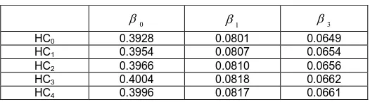
Robust Covariance Matrix Estimation can be used for testing heteroskedasticity. We can see that standard errors given different types of HC (Heteroscedasticity), based on [4] , there is no heteroskedasticity in Fixed Effects model and Random Effects Model, is given in the following table 5 and table 6.
Table 5.
Controlling for Heteroskedasticity:Fixed Effects
1
2 3 4
HC0 0.1196 0.0724 0.0644 0.0842
HC1 0.1206 0.0733 0.0650 0.0849
HC2 0.1216 0.0737 0.0655 0.0855
HC3 0.1236 0.0747 0.0666 0.0869
HC4 0.1242 0.0750 0.0667 0.0874
Table 6.
Controlling for Heteroskedasticity: Random Effects
0
1 3
HC0 0.3928 0.0801 0.0649
HC1 0.3954 0.0807 0.0654
HC2 0.3966 0.0810 0.0656
HC3 0.4004 0.0818 0.0662
HC4 0.3996 0.0817 0.0661
4. ESTIMATION RESULTS
It can be seen from the overall results of the analysis above, that models A and B were obtained that met the results of the diagnostic test. To determine which model is best presented through table 7 below
Table 7.
Fixed effects and Random Effects models : Estimation results
MODEL A ( Fixed-Effect Model with Individual effect):
t i i c X X
X X
it
Y ,
5 log 5 3 log 3 2 log 2 1 log 1
log
Coefficients Estimate Std. Error t-value Pr(>|t|) 1
0.419731 0.093715 4.4788 1.216e-05 ***
2
0.171607 0.071369 2.4045 0.01704 *
3
0.543294 0.041771 13.0064 < 2.2e-16 ***
5
-0.747976 0.078490 -9.5295 < 2.2e-16 ***
Residual Sum of Squares 2.3726
Adj. R-Squared 0.95054
F-statistic 1103.48
p-value < 2.22e-16
MODEL B (Random Effect Model with two-way effect/Individual effect and time effect) t
i t d i c X X
it
Y ,
3 log 3 1 log 1
log
Coefficients Estimate Std. Error z-value Pr(>|t|)
(Intercept) 0.833420 0.225393 3.6976 0.0002176 ***
1
0.479763 0.047238 10.1564 < 2.2e-16 ***
3
0.606135 0.038210 15.8633 < 2.2e-16 ***
Residual Sum of Squares 3.5669
Adj. R-Squared 0.93438
Chisq 3262.73
322
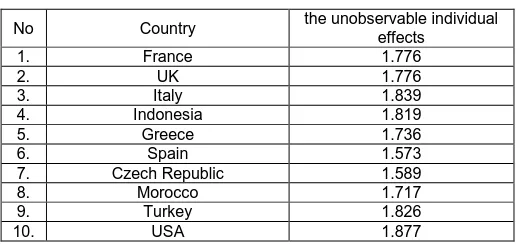
Table 8.
the unobservable individual effects for each Country
No Country the unobservable individual effects
1. France 1.776
2. UK 1.776
3. Italy 1.839
4. Indonesia 1.819
5. Greece 1.736
6. Spain 1.573
7. Czech Republic 1.589
8. Morocco 1.717
9. Turkey 1.826
10. USA 1.877
By looking at the value of the Residual Sum of Squares (RSS) of each model, where for models A=2.3726 and model B=3.5669, based on the principle of simplicity or Parsimony that by viewing the minimum of RSS value. It can be concluded that model A is the most appropriate model. We can see also, the value of Adj. R-Squared for model A =0.95054 higher than the value of Adj. R-Squared for model B=0.93438. We found that model A (Fixed Effects Model with Individual effect) is the best panel model, with values of the unobservable individual effect (Ci) for each country
presented in table 8. In table 7, for model A, where 1, 2
3
and are all significant (t-value> Pr(>|t|) ), this implies that
the positive effect on Gross Domestic Product (GDP) arising from Number of International tourist arrivals; International Tourism Receipts ; and International Tourism Expenditures, although the negative effect on Gross Domestic Product arising from Total Employment in tourism sector ,where 5 is
also significant (t-value < Pr(>|t|) ) Furthermore, Adj. R-Squared = 0.95054 and F-statistic = 1103.48 (p-value =< 2.22e-16), this implies that all independent variables are adjusted together explain the variable GDP (dependent variable) by 95,054% while the remaining 4.946% is explained by other variables outside the model and all independent variables are statistically significant at a = 5% which means all independent variables have a significant influence on the GDP variable.
5. CONCLUSIONS
1).Based on panel data analysis method, the most appropriate model is the Fixed Effects model with
Individual Effects
) log
0.75 log 0.54 log 0.17 log 0.42
(log Yit X1 X2 X3 X5cii,t
where the values of ci (Unobservable Individual Effects)
for each countries such as France (1,776); UK(1.776); Italy(1.839); Indonesia(1.819); Greece(1.736); Spain(1.573); Czech Rep.(1.589); Morocco(1.717); Turkey(1.826) and USA(1.877) respectively.
2) Based on the F test, the Number of International Tourist Arrivals, International Tourism Receipts, International Tourism Expenditures, and Total Employment in the tourism sector, have a simultaneous significant influence on The Gross Domestic Product (GDP). Results of this study shows that the International Tourist Arrivals, International Tourism Receipts, International Tourism Expenditures, and Total Employment in tourism sectors as
factors that can explain changes in Domestic Products Gross (GDP) from France, UK, Italy, Indonesia, Greece, Spain, Czech Rep., Morocco, Turkey, and the USA. 3) Based on the t-test, the number of International Tourist
Arrivals, International Tourism Receipts, and International Tourism Expenditures, has a partial positive impact that is significant to the Gross Domestic Product (GDP). Results of this study reveal that the Number of International Tourist Arrivals, International Tourism Receipts, and International Tourism Expenditures, as factors that can explain changes in the Gross Domestic Product (GDP) from France, UK, Italy, Indonesia, Greece, Spain, Czech Rep., Morocco, Turkey, and the USA.
4) Based on the t-test, Total Employment in the tourism sector has a partial negative impact that is significant to the Gross Domestic Product (GDP). The results of this study show that Total Employment in the tourism sector as a factor that can explain changes in the Gross Domestic Product (GDP) from France, UK, Italy, Indonesia, Greece, Spain, Czech Rep., Morocco, Turkey, and the USA. Its surprising results that may reveal the possibility of unreported transactions, low payment to increased employment and the black market in the sector that does not reflect the reality of employment contribution to the Gross Domestic Product (GDP).
5) Based on Adj.R square, this implies that the Number Of International Tourist Arrivals, International Tourism Receipts, International Tourism Expenditures, and Total Employment in the tourism sector, adjusted together explain the Gross Domestic Product (GDP) by 95.054% from France, UK, Italy , Indonesia, Greece, Spain, Czech Rep., Morocco, Turkey, and the USA while the remaining 4.946% is explained by other variables outside the model. 6) Future research can modify this panel model by adding
some dummy variables and use that model for forecasting purposes related to applications in tourism demand.
REFERENCES
[1] Baltagi, BH Econometric Analysis of Panel Data.Chichester:Wiley. 2013.
[2] Brida, J. G., & Risso, W. A. A dynamic panel data study of the German demand for tourism in South Tyrol. tourism and Hospitality Research, 9(4), 305-313. 2009.
[3] Carey,K.. Estimation of Carribean Tourism Demand: Issues in Measurement and Methodology. Atlantic Economy Journal, 19,32-40. 1991.
[4] Croissant, Y., & Millo, G. Panel Data Econometrics in R: The plm Package." Journal of Statistical Software, 27(2). 2008 URL http://www.jstatsoft.org/v27/i02/ [5] Garin-Munoz, T. Inbound international tourism to
Canary Islands: A dynamic panel data model. Tourism Management, 27(2), 281-291. 2006.
[6] Garin-Munoz, T., & Montero-Martin, L. F.. Tourism in the Balearic Islands: A dynamic model for international demand using panel data. Tourism Management, 28(5), 1224-1235. 2007
[7] Greene, W.H. Econometric Analysis. Prentice Hall, New Jersey. 2003.
323 [9] Hsiao, C.. Analysis of Panel Data.Cambridge:
Cambridge University Press. 1986.
[10] Kuo, H.-I., Chang, C.-L., Huang, B.-W., Chen, C.-C., & McAleer, M.. Estimating the impact of Avian Flue on international tourism demand using panel data. Tourism Economics, 15(3), 501-511. 2009.
[11] Ledesma-Rodriguez, F. J., & Navarro-Ibanez, M.. Panel data and tourism: A case study of Tenerife. Tourism Economics, 7(1), 75-88. 2001.
[12] Lim,C. An Econometric Classification and Review of International Tourism demand Models. Tourism Economics, 3.69-81.1997
[13] Naude, W. A., & Saayman, A. Determinants of tourist arrivals in Africa: A panel data regression analysis. Tourism Economics, 11(3), 365-391. 2005.
[14] Romilly, P., Liu, X., & Song, H. Economic and social determinants of international tourism spending: A panel data analysis. Tourism Analysis, 3(1), 3-16.1998. [15] Sakai,M., Brown,J., and Mak, J. Population aging and
Japanese International Travel in the 21st century. Journal of Travel Research, 38, 212-220. 2000.
[16] Taylor, T., & Ortiz, R. A. Impacts of climate change on domestic tourism in the UK: A panel data estimation. Tourism Economics, 15(4), 803-812. 2009.