DEVELOPMENT AND STATISTICAL VALIDATION OF A SIMPLIFIED
LOGISTIC LAND USE CHANGE MODEL
Tahmina Khan1, Michael Anderson2
1,2 Civil and Environmental Engineering Department, the University of Alabama in Huntsville, USA
Received 6 June 2016; accepted 5 August 2016
Abstract: Landscapes are dynamic, and the driving forces towards the societal change are related to the population growth and the lifestyle becoming increasingly urban and more mobile. The efforts to understand patterns and driving forces of urban growth or expansion have been analyzed in previous and recent studies. There is no doubt that the demand for urban land and the pressure for sustainable development will increase in any Metropolitan Area in the near future. In this study, land use change models were derived with and without variables related to urban sprawl and compared based on their statistical significance. The main goal of this paper is to propose a simplified logistic model, tested in Huntsville, AL that can highlight the probability of land use change by Traffic Analysis Zone (TAZ). Validation approach demonstrates the applications of measures of discrimination and calibration for a logistic regression model. This study can help to improve the understanding of patterns and determinants of urban growth and land expansion in Huntsville, AL. The model can be very useful to forecast the future probability of land use change and can be a substantial input in planning and decision-making process.
Keywords:land use change model, logistic regression, statistical validation, probability of land use change, traffic analysis zone.
1 Corresponding author: [email protected]
1. Introduction
Landscapes are dynamic, and all the important driving forces towards the societal change are related to the population growth and the lifestyle becoming increasingly urbaner and more mobile. The three main driving forces such as accessibility, urbanization, and globalization that affected the nature and pace of the changes as well as the perception people have had about the landscape (Antrop 2005). During the last decades, high rates of change causing unsustainable development have attracted the attention of policy and planning and raised
the need to understand the factors behind it. The road network shows a continuous growth and the built-up area a continuous expansion, both corresponding to positive transformation rates that mean both contribute an increase in respective landscape elements (Schneeberger et al., 2007).
patterns, income levels, car ownership trends, infrastructure investment, regional economic dynamics, etc. also may lead to congestion. Uncontrolled urban expansion or urban sprawl is a serious threat to urban sustainability and hence, poses a huge challenge to researchers, urban planners and policy makers to come up with remedial solutions (Mukherjee et al., 2014), (Rao and Rao, 2012).
Huntsville is the fastest growing major metro area in the state of Alabama, accounted for 34% of Alabama’s Growth in population, and employment growth exceeds Alabama as a whole. The community and local business owners continue to be very positive, and the trend toward new growth is inevitable (COCH, 2015). The efforts to understand patterns and driving forces of urban growth or expansion have been analyzed in previous and recent studies, due to the intensified consequences of human activities on resources, open spaces, and the environment. The rapid growth can be accompanied by the disappearance of rural agricultural land, spatial fragmentation, and sustainability challenges (Luo and Wei, 2009). There is no doubt that the demand for urban land and the pressure for sustainable development will increase in Huntsville in the near future. Better understanding and managing of urban growth are critical to the development and sustainability in any city.
In this study, land use change models were derived with and without the variables related to urban sprawl and compared based on their statistical significance. The main goal is to propose a simplified logistic
model for Huntsville that can highlight the probability of land use change by Traffic Analysis Zone (TAZ). The model performance was assessed through different statistical measures. Validation approach demonstrates the applications of measures of discrimination and calibration for a logistic regression model. This study can help to improve the understanding of patterns and determinants of urban growth and land expansion in Huntsville. The model can be very useful to forecast the future probability of land use change and can be a substantial input in planning and decision-making process.
2. Literature Review
Spatial distribution of future land use is related to demand and development supply, accessibility, spatial suitability of each piece of land, and decision-making results of different decision-makers such as households, employment, governments, land owner, and developers. It is required to know the land use variables used in recent Land Use models that can be outlined as follows:
• Bid-Rent- Analytical models based on real estate pricing, and utility maximization theory (Clay et al., 2011)
º Bid rent model is a geographical-economic theory that refers to how the price and demand of real estate change with distance (Zhao and Peng, 2010)
• Gravity/Logit- Analytical models founded on the concept of spatial separation (Clay et al., 2011)
• Microsimulation- Analytical models that use Monte Carlo and other simulation techniques (Clay et al., 2011) • Rule-Based- Those models that use rule-based decision trees (Clay et al., 2011) • An Integrated Bi-Level Model (Land
Use/Transportation Model) - Cellular automata (CA) along with agent-based model capture the spatial drivers, human behaviors, and socioeconomic characteristics of land use change (Zhao and Peng, 2010)
Other variables explored were those related to the construction costs and developer choices, with respect to land use within the model. Factors with potentially significant impact on land use include (Clay et al., 2011):
• Construction economy
• Development and chronolog y of “dependent” land use
• Soil conditions & Availability of utilities • Planning & zoning
• Municipal (or other) incentives (or disincentives) that impact development
The recent land use models/strategies that focus on human behaviors, socioeconomic characteristics, distance, price/cost and uncertainty involved in making the decision for implementing a new development (new household/new employment). It is understandable that the models above
are not appropriate to address our issue while a simple model can estimate the likelihood of land use change for each TAZ in Huntsville. Moreover, models can be compared with or without variables used in scoring urban sprawl and can be applied to solve our stated problem. Because time and resources required gathering data along with the building of specific model is the major impediment, it is necessary to look at prevailing land use change model and the factors or driving forces responsible for land use change.
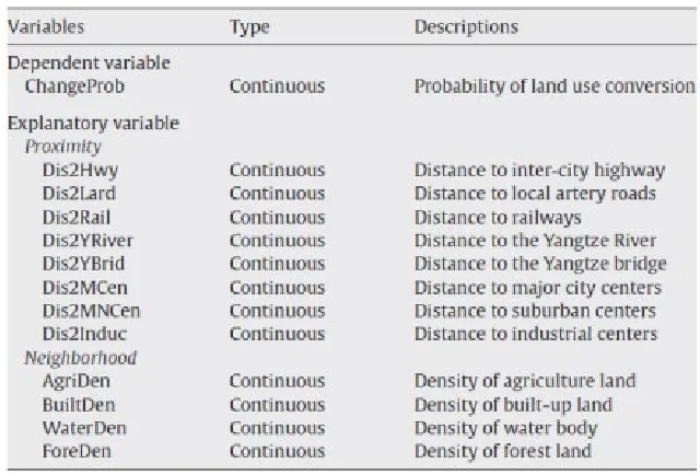
Fig. 1.
Variables Used in the Land use Conversion Models Source: (Luo and Wei, 2009)
The case study analyzed in later section uses the classic multivariate statistic analysis in the modeling of land expansion. To quantify the influences of explanatory variables on probability of urban land expansion, the classic logistic regression takes the following forms (Luo and Wei, 2009), Eq. (1) and Eq. (2):
(1)
(2)
Where: ChangeProb: the probability of land-use change to be regressed at location i, C: constant, βk is the parameter for individual explanatory variable Xki (k=1, 2, 3,……, n) that includes both socio-economic and spatial data. This classic logistic regression
model adequately explains the determinants of the probability of urban land expansion from the global view (Luo and Wei, 2009).
3. Case Study
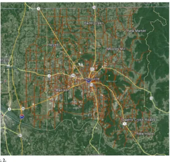
Fig. 2.
Picture of Study Area
Source: (Screenshot of Google map)
Following sections contain several essential parts to explain the response/dependent variable and explanatory variables, analysis and results, and validation process.
4. Data/Variables
Data were collected mostly from US census
for the year 2000 and 2010. The variables can be divided into two broad categories as follows:
4.1. Independent Variables
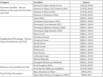
Table 1
Explanatory Variables
Category Variables Source
Proximity Variables - Nearest distance to the respective item from each TAZ
Distance to Major Roads in Feet (USCB, 2010) Distance to Major City Centers in Feet (USCB, 2010) Distance to River in Feet (USCB, 2010) Distance to Railways in Feet (USCB, 2010)
Neighborhood Percentage - Percent Type of Landuse for each TAZ
Open Water (MRLC, 2016)
Developed, Open Space (DO) (MRLC, 2016) Developed, Low Intensity (DL) (MRLC, 2016) Developed, Medium Intensity (DM) (MRLC, 2016) Developed, High Intensity (DH) (MRLC, 2016)
Barren Land (MRLC, 2016)
Deciduous Forest (MRLC, 2016) Evergreen Forest (MRLC, 2016)
Mixed Forest (MRLC, 2016)
Shrub/Scrub (MRLC, 2016)
Herbaceous (MRLC, 2016)
Hay/Pasture (MRLC, 2016)
Cultivated Crops (MRLC, 2016)
Woody Wetlands (MRLC, 2016)
Emergent Herbaceous Wetlands (MRLC, 2016) Measures of Accessibility by TAZ Road Length in Miles (USCB, 2010) Road density (Miles per Sq Miles) (USCB, 2010)
Zonal Surface Parameters Mean Elevation in MeterMean Slope Percent (45 degree is 100%) DEM, 2015 DEM, 2015
Refined versions of the indices capture four distinct dimensions of sprawl for instance development density, land use mix, population and employment centering, and street accessibility. Compactness indices/ sprawl-like metrics for census tracts within metropolitan areas were derived through the use of following variables together with the equations (shown in Table 2 and Table 3) as in larger area analyzes (metropolitan area, urbanized area, and county sprawl metrics) (Ewing and Hamidi, 2014). These variables used in urban sprawl indexing were employed to develop another model that can be compared with the previous model. Because of unavailability of Walk Score related data, a new variable was introduced to measure the walkability. From any grocery
shop to a TAZ block, if the nearest distance is within 1.5 miles, those values were inversed and weighted by the sum of block level population and employment as a percentage of the TAZ total to obtain Grocery/Amenity reachability index.
that included a total number of jobs and the number of employment by two-digit NAICS (North American Industry Classification
System) code. The data were aggregated to generate total jobs by one-digit NAICS code for every block under any particular TAZ.
Table 2
Variables Used in Measuring Sprawl Indices
Category Variables Source
Density Factor Gross Population densityGross Employment density (USCB, 2010), (ESRI, 2004)(LED, 2015)
Mix Use Factor
Job-Population balance (USCB, 2010), (LED, 2015), (ESRI, 2004)
Degree of Job mixing (LED, 2015)
Grocery/Amenity reachability index (USCB, 2010), Google Earth
Street Factor
Intersection density (USCB, 2010)
% 4 or more way intersection (USCB, 2010) Average Block Size (USCB, 2010), (ESRI, 2004) Percent of Small blocks (<1/100 sq miles) (USCB, 2010), (ESRI, 2004)
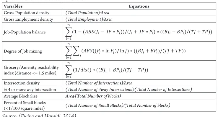
Table 3
Equations to Determine New Variables2
Variables Equations
Gross Population density (Total Population)⁄Area
Gross Employment density (Total Employment)⁄Area
Job-Population balance
Degree of Job mixing
Grocery/Amenity reachability index (distance <= 1.5 miles)
Intersection density (Total Number of Intersections)⁄Area
% 4 or more way intersection (Total Number of 4way Intersections)⁄(Total Number of Intersections)
Average Block Size Area⁄(Total Number of blocks)
Percent of Small blocks
(<1/100 square miles) (Total Number of Small Blocks)⁄(Total Number of blocks) Source: (Ewing and Hamidi, 2014)
2 Where, i is the census block number, n is the number of blocks in the TAZ, J
i or BJi is jobs in census block, Pi or BPi is residents in census block, JP is jobs per person in the metropolitan area, TJ is the total jobs in the TAZ, Pj is proportion of jobs in sector j, and j is the number of sectors.
4.2. Dependent Variable
National Land Cover Database (NLCD) serves as the definitive Landsat-based, 30-meter resolution, land cover database
2014). It provides not only land cover data (LCD) by year (2001 or 2011) but also land cover change data (LCCD) from the year 2001 to 2011. The total area for a particular type of development can be summarized at TAZ level using ArcGIS. Based on the relative probability of development or the percent developed between 2001 and 2011 can be a good estimator to identify the necessary dependent variable. Table 1 shows different types of development classified by NLCD.
It is needed to understand the raster database involved above colored features
that can provide the likelihood estimates of development between 2001 and 2011. Since it is a binary logistic regression model, the estimation of dependent variable which is either 0 or 1 must be done in a very conservative manner. For instance, DO or DL for some TAZs cannot represent the development concentration as much as DM and DH can. Therefore, a three level of estimation of likelihood can be considered where DO and DL can be ruled out to show the high-density development. After that, to determine the extent of development occurred, the following measures were calculated for all TAZs.
Table 4
Measures of Development
Intensity Inclusion Type Probability of Land Use Change Percent Change
Low DO+DL+DM+DH Ratio of Land Cover Change Data (between 2001 and 2011) by TAZ to that of total for the study area
Ratio of Land Cover Change Data (between 2001 and 2011) by TAZ to 2001 Land Cover Data by respective TAZ
Medium DL+DM+DH Ratio of Land Cover Change Data (between 2001 and 2011) by TAZ to that of total for the study area
Ratio of Land Cover Change Data (between 2001 and 2011) by TAZ to 2001 Land Cover Data by respective TAZ
High DM+DH Ratio of Land Cover Change Data (between 2001 and 2011) by TAZ to that of total for the study area
Ratio of Land Cover Change Data (between 2001 and 2011) by TAZ to 2001 Land Cover Data by respective TAZ
At this point, it is needed to rank each TAZ based on the percentiles of above measures. Since binary logistic regression requires 0 and 1 value as the response variable, the ranking was implemented at 50 percentile value of each measure for the study area. For instance, if a TAZ value falls below 50 percentile value of a particular measure, 0 was assigned against that TAZ and vice versa. Overall rank was chosen by the mode of all ranks so that the ranking of six measures can be summarized into one dimension. Doing this yields a number (either 0 or 1) to represent the approximate likelihood of development by TAZ, that means, higher the value, more expansion can be expected by a TAZ.
5. Analysis and Results
This section describes model development procedure and comparison of preliminary and final models.
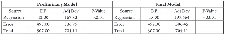
Table 5
Deviance Table
Preliminary Model Final Model
Source DF Adj Dev P-Value Source DF Adj Dev P-Value Regression 12.00 167.32 <0.01 Regression 15.00 197.664 <0.001
Error 495.00 536.79 Error 492.00 506.45
Total 507.00 704.11 Total 507.00 704.11
Deviance Table (See Table 5) displays the likelihood ratio test p-values for the coefficients. The p-value for the overall regression tests the null hypothesis that all the coefficients for predictors are equal to zero. The alternative hypothesis is that at least one of the coefficients for a predictor is not equal to zero (Minitab, 2015). Here, the p-value is close to zero. This p-value indicates that there is sufficient evidence that at least one of the coefficients is different from zero in both models. However, deviance of final model is less than that of preliminary
because of additional variables, and a smaller value of deviance indicates an improvement in fit.
Model Summary (See Table 6) displays the statistics to compare how well different models fit the data. Higher values of deviance R-Sq and adjusted deviance R-Sq indicate a better fit while smaller values of Akaike Information Criterion (AIC) indicate a better fit (Minitab, 2015). The preliminary model does not have better-fit statistics comparing to the final model.
Table 6
Model Summary
Model Deviance R-Sq Deviance R-Sq(adj) AIC
Preliminary 23.76% 22.06% 562.79
Final 28.07% 25.94% 538.45
R eg re s sion E qu at ion d i s pl ay s t he transformation that changes the linear equation into a predicted probability and a linear equation for predictors that includes continuous variables after eliminating insignificant variables at an alpha level of 0.15.
Regression Equation, Eq. (3) and Eq. (4):
(3)
(4)
Preliminary Model
Y’= 0.02 - 0.000031 Distance to Major Roads in Feet - 0.000020 Distance to River in Feet - 7.93 Open Water + 2.63 Developed, Open Space - 2.60 Developed, High Intensity
+ 9.17 Shrub/Scrub - 6.18 Woody Wetlands + 0.0615 Road Length in Miles
Final Model
Y’ = 1.46 - 0.000025 Distance to Major Roads in Feet - 0.000019 Distance to River in Feet - 10.09 Open Water - 5.21 Developed, High Intensity - 1.371 Cultivated Crops - 6.60 Woody Wetlands + 0.0865 Road Length in Miles + 0.02322 Mean Elevation in Meter - 0.2714 Mean Slope Percent - 0.000033 Distance to Major City Centers in Feet - 0.2211 Road density - 0.000615 Gross Population density - 0.000248 Gross Employment density + 2.514 Degree of Job mixing - 5.52 Average Block Size
The primary tool for most process modeling applications is summary measures of goodness-of-fit from a fitted model that provide
information on the adequacy of different aspects of the model. The logistic regression with binary data is the area in which graphical residual analysis can be difficult to interpret as a model validation (Rana et al., 2010).
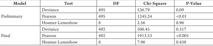
Table 7 for Goodness-of-Fit Tests displays Pearson, deviance, and Hosmer-Lemeshow goodness-of-fit tests. The goodness-of-fit tests excluding Pearson, with p-values ranging from 0.09 to 0.96 that are greater than an alpha-level of 0.05, indicate that there is insufficient evidence to claim that the model does not fit the data adequately. Since two out of three tests fail to reject the null hypothesis of an adequate fit, it can be concluded that both models are well fitted and valid (Minitab, 2015).
Table 7
Goodness-of-Fit Tests
Model Test DF Chi-Square P-Value
Preliminary
Deviance 495 536.79 0.09
Pearson 495 1245.24 <0.01
Hosmer-Lemeshow 8 2.56 0.96
Final
Deviance 492 506.45 0.317
Pearson 492 1913.53 <0.001
Hosmer-Lemeshow 8 7.96 0.438
Based on the above statistics, it can be stated that model with sprawling variables presents a better fit. It can be observed that new variables exert a great impact on urban expansion specially Average Block Size and Degree of Job Mixing. The final model effectively explains the determinants of the probability of urban land expansion. The sprawling nature of Huntsville is somewhat reflected from our logistic model.
6. Statistical Validation
Since the fitted model performs in an optimistic manner on the fitting sample, it
stringent and unbiased test for the model and the entire data collection process. However, it is not possible to obtain a new independent external sample from the same population or a similar one. That leads to doing an internal validation of the model which includes several accredited methods such as data-splitting, repeated data-data-splitting, jackknife technique and bootstrapping, etc. The core concept of these methods is to exclude a subsample of observations, develop a model based on the remaining subjects, and then test the model in the originally excluded subjects (Giancristofaro and Salmaso, 2003).
Here, the repeated data splitting approach was implemented where data were split
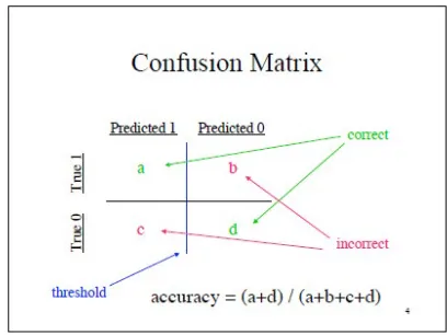
randomly into the fitting and validation samples without replacement by 75% and 25% respectively. The fitting sample is used to fit the model while the validation sample is used to evaluate its performance based on a two by two table known as confusion matrix. Logistic regression was performed for 10 times, and the average values were determined to propose the ultimate land use change model since each iteration is based on a different split of the original data, it results in different model coefficients, significance levels, and performance values (Giancristofaro and Salmaso, 2003). Confusion matrix outlined as follows was determined using MATLAB to validate the model (MathWorks, 2015).
Fig. 3.
Confusion Matrix
To assess the model’s quality of fit, the distributions of the estimates need to be averaged around the same values as the estimates computed on the whole original sample. If this does not happen, the model cannot be validated because of its internal instability.
6.1. The Model’s Quality of Fit
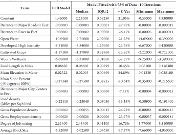
Table 8
Quality of the Model’s Fit: Stability of the Parameters’ Estimates
Term Full Model Model Fitted with 75% of Data - 10 Iterations
Median IQR/2 ~ C Var Minimum Maximum
Constant 1.46000 2.23000 0.69250 31.05% -0.53000 3.830000 Distance to Major Roads in Feet -0.00003 -0.00003 0.00001 -27.78% -0.00004 -0.000015 Distance to River in Feet -0.00002 -0.00002 0.00000 -26.47% -0.00003 -0.000011 Open Water -10.0900 -9.75000 2.07000 -21.23% -14.69000 -0.390000 Developed, High Intensity -5.21000 -5.34000 1.27000 -23.78% -6.67000 0.420000 Cultivated Crops -1.37100 -1.37900 0.32900 -23.86% -2.22000 -0.722000 Woody Wetlands -6.60000 -6.21000 2.01000 -32.37% -9.25000 -3.390000 Road Length in Miles 0.08650 0.08600 0.00899 10.45% 0.06100 0.116300 Mean Elevation in Meter 0.02322 0.02005 0.00499 24.89% 0.01230 0.038100 Mean Slope Percent
(45 degree is 100%) -0.27140 -0.27590 0.02935 -10.64% -0.35000 -0.216600 Distance to Major City Centers
in Feet -0.00003 -0.00003 0.00000 -7.35% -0.00004 -0.000025 Road density
(Miles per Sq Miles) -0.22110 -0.23040 0.03030 -13.15% -0.30900 -0.191400 Gross Population density -0.00062 -0.00055 0.00013 -24.22% -0.00081 -0.000413 Gross Employment density -0.00025 -0.00025 0.00006 -23.67% -0.00037 -0.000184 Degree of Job mixing 2.51400 2.45400 0.41100 16.75% 1.77000 3.510000 Average Block Size -5.52000 -6.02500 1.04650 -17.37% -7.66000 -4.030000
Where, IQR/2 is half of the interquartile range, C Var is the ratio between IQR/2 and the Median.
The variability is moderate, indicating the presence of some degree of overfitting. As the model validates outside the available sample, the parameter’s estimates computed on the full sample has been used by Eq. (1), Eq. (2) and Y’ (Final Model).
Table 9 presents the overall significance of the model and the partial significance of each of the covariates. Again, both the information related to the full model and the information describing the fitting
Table 9
Quality of the Model’s Fit: Significance
Item Full Model Model Fitted with 75% of Data - 10 Iterations
Median IQR/2 ~ C Var Minimum Maximum
Regression <0.001 <0.001 <0.001 No Change <0.001 <0.001 Distance to Major Roads in Feet 0.051 0.0755 0.11125 147.35% 0.017 0.343 Distance to River in Feet 0.003 0.0265 0.02925 110.38% <0.001 0.118 Open Water 0.048 0.0830 0.15000 180.72% 0.012 0.960 Developed, High Intensity 0.004 0.0290 0.13650 470.69% 0.001 0.881 Cultivated Crops 0.110 0.1690 0.10365 61.33% 0.037 0.451 Woody Wetlands 0.011 0.0285 0.05900 207.02% 0.003 0.312 Road Length in Miles <0.001 0.0010 0.00200 200.00% <0.001 0.016 Mean Elevation in Meter 0.008 0.0475 0.04400 92.63% <0.001 0.249 Mean Slope Percent
(45 degree is 100%) <0.001 <0.001 <0.001 No Change <0.001 <0.001 Distance to Major City Centers
in Feet <0.001 <0.001 <0.001 No Change <0.001 0.002 Road density
(Miles per Sq Miles) <0.001 <0.001 <0.001 No Change <0.001 <0.001 Gross Population density <0.001 0.0020 0.00213 106.25% <0.001 0.018 Gross Employment density 0.002 0.0065 0.01875 288.46% <0.001 0.073 Degree of Job mixing 0.005 0.0160 0.02500 156.25% 0.001 0.088 Average Block Size 0.001 0.0025 0.01225 490.00% 0.001 0.055
6.2. Generalizability of the Model
In order for the model to be validated, model performance was assessed by comparing the actual value to the predicted one through the use of the following measures.
In all cases for determining the ability of the model to distinguish correctly the two classes of outcomes (confusion matrix), the accuracy was more than 70% for the validation sample when the cutoff point or threshold was 0.5 to classify the predicted probabilities.
A widely used statistic produced by Hosmer and Lemeshow to test the ability of a given
model to calibrate, has the following format (Giancristofaro and Salmaso, 2003), Eq. (5):
(5)
Where: nj, Oj, and Pj are respectively the number of observations, the number of positive outcomes (value of 1) and the average predicted probabilities for the jth group.
probabilities are to the observed rate of the positive outcome. If an observed Chi-squared value less than the critical value of the Chi-squared distribution with Q-2 degrees of freedom at 0.05 alpha level, indicates good calibration (Giancristofaro and Salmaso, 2003).
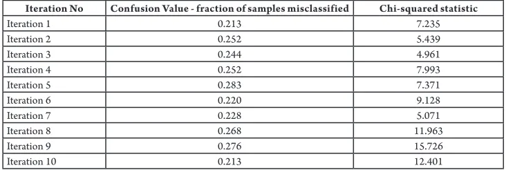
Estimated Chi-square value is smaller than the critical value with 8 degrees of freedom for all iterations at an alpha level of 0.05 (that is 15.51) except for one iteration (shown in Table 10). It can be interpreted that the calibration on the validation samples is excellent.
Table 10
Amount of Misclassification and Hosmer and Lemeshow Test Statistic
Iteration No Confusion Value - fraction of samples misclassified Chi-squared statistic
Iteration 1 0.213 7.235
Iteration 2 0.252 5.439
Iteration 3 0.244 4.961
Iteration 4 0.252 7.993
Iteration 5 0.283 7.371
Iteration 6 0.220 9.128
Iteration 7 0.228 5.071
Iteration 8 0.268 11.963
Iteration 9 0.276 15.726
Iteration 10 0.213 12.401
7. Conclusions
The purpose is to build a simplified logistic model for Huntsville that can highlight the probability of land use change by Traffic Analysis Zone (TAZ). To do so, land use change models were derived with and without the variables related to urban sprawl and compared based on their statistical significance. The model with sprawling variables presents a better fit and effectively explains the determinants of the probability of urban land expansion. The sprawling nature of Huntsville is somewhat reflected from our logistic model.
It can be observed that new variables exert a great impact on urban expansion specially Average Block Size and Degree of Job Mixing. Other common variables, such as the proximity variables have minor effects on land conversion probability. Among neighborhood
percentage variables, Open Water has the strongest negative effect on land conversion probability, followed by Woody Wetlands, Developed, High Intensity and Cultivated Crops. It can suggest that these variables restrict urban land expansion. Altogether, neighborhood and proximity variables imply that large-scale urban land development is not highly dependent on existing development or urban centers. Among zonal and accessibility variables, Slope and Road Density have greater influence than Road Length and Elevation. It has been found that the model with new variables is more significant (especially variables Average Block Size and Degree of Job Mixing) and should be included in developing land use change model for other location.
use trend since it balances between two dimensions of performance namely measure of discrimination and calibration in order to find the best trade-off.
Finally, this model can be utilized to forecast the likelihood/probability of land use change at TAZ level (such as 2020) since independent variables (such as 2010) are easily obtainable. The results can be useful in updating Travel Demand Models or Land Use Models, thus, it can help planners and decision makers in articulating and comparing different planning scenarios.
References
Antrop, M. 2005. Why landscapes of the past are important for the future, Landscape and urban planning, 70(1): 21-34.
Clay, M.J.; W hite, W.L.; Holley, P. 2011. Data Development for Implementing an Integrated Land Use and Transportation Forecasting Modeling in a Medium-Sized MPO. In Proceedings of Transportation
Research Board 90th Annual Meeting.
COCH. 2015. 2015 State of the Economy-The Chamber of Commerce of Huntsville/Madison County. Available from internet: <http://www.huntsvillealabamausa.com/>.
DEM. 2015. Digital Elevation Model. AlabamaView. Accessed December 10, 2015. Available from internet: <http://www.alabamaview.org/DEM.php>.
ESRI. 2004. ESRI Data & Maps-ArcGIS 9 Media Kit. Redlands, CA: ESRI.
Ewing, R.; Hamidi, S. 2014. Measuring urban sprawl and validating sprawl measures. Available from internet: <https://gis.cancer.gov/tools/urban-sprawl/sprawl-report-short.pdf >.
Giancristofaro, R.A.; Salmaso, L. 2007. Model performance analysis and model validation in logistic regression, Statistica, 63(2): 375-396.
Han, J.; Hayashi, Y.; Cao, X.; Imura, H. 2009. Application of an integrated system dynamics and cellular automata model for urban growth assessment: A case study of Shanghai, China, Landscape and Urban
Planning, 91(3): 133-141.
LED. 2015. Longitudinal Employer-Household Dynamics. Local Employment Dynamics. Accessed December 10, 2015. Available from internet: <http:// lehd.ces.census.gov/data/>.
Luo, J.;Wei, Y.D. 2009. Modeling spatial variations of urban growth patterns in Chinese cities: the case of Nanjing, Landscape and Urban Planning, 91(2): 51-64.
MathWorks. 2015. MATLAB and Statistics Toolbox Release 2015a. The MathWorks, Inc.Massachusetts, United States.
Minitab. 2015. Minitab Statistical Software, Release 17. Available from internet: <https://www.minitab. com/en-us/>.
MRLC. 2016. National Land Cover Database. Multi-Resolution Land Characteristics (MRLC) Consortium. Available from internet: <http://www.mrlc.gov/ finddata.php>.
Mukherjee, A.B.; Pate, N.; Krishna, A.P. 2014. Development of heterogeneity index for assessment of relationship between land use pattern and traffic congestion, International Journal for Traffic & Transport
Engineering, 4(4): 397-414.
Rana, S.; Midi, H.; Sarkar, S.K. 2010. Validation and performance analysis of binary logistic regression model.
In Proceedings of the WSEAS International Conference on
Rao, A.M.; Rao, K.R. 2012. Measuring urban traffic congestion-a review, International Journal for Traffic and
Transport Engineering, 2(4): 286-305.
Schneeberger, N.; Bürgi, M.; Hersperger, A.M.; Ewald, K.C. 2007. Driving forces and rates of landscape change as a promising combination for landscape change research-An application on the northern fringe of the Swiss Alps, Land Use Policy, 24(2): 349-361.
USCB. 2010. Tiger/Line Shapefiles. United States Census Bureau. Available from internet: <https:// www.census.gov/geo/maps-data/data/tiger-line.html>.
Zhao, L.; Peng, Z-R. 2010. An Integrated Bi-Level Model to Explore the Interaction between Land Use Allocation and Transportation, Transportation Research Record: Journal