Stability and Convergence Analysis of Smoking Impact in Society with Algorithm Aspects

(1)

Volume 17, Number 4 (2019), 503-516

URL:https://doi.org/10.28924/2291-8639 DOI:10.28924/2291-8639-17-2019-503

STABILITY AND CONVERGENCE ANALYSIS OF SMOKING IMPACT IN SOCIETY WITH ALGORITHM ASPECTS

AQEEL AHMAD∗, MARYAM SHAHID, MUHAMMAD FARMAN, M.O. AHMAD

Department of Mathematics and Statistics, The University of Lahore, Lahore, Pakistan

∗_{Corresponding author:} _{[email protected]}

Abstract. In this manuscript, an epidemic model employed the dynamics of drugs usage among adults. Among smokers, often the desire to quit smoking arises. A large number of smokers attempt to quit, but only a few of them are successful. A non-linear mathematical model is employed to study and assess the dynamics of smoking and its impact on public health in a community. We prove the essential properties, bounded, positivity and well-posed, also local and global stability analysis has been made for the epidemic model. The sensitivity analysis of the model is provided by threshold or reproductive number as well as analyzed qualitatively. We develop an unconditionally convergent nonstandard finite difference scheme by applying Mickens approachφ(h) =h+O(h2) instead ofhto control the spread of bad impact in society. Finally numerical simulations are also established to investigate the influence of the system parameters on the spread of the smoking impact in society.

1. _Introduction

The scope of mathematics includes mathematical modeling and esoteric mathematics. The flow of work,

process, predictions and outcomes can easily be measured with the help of mathematical concepts and

theories. Therefore, biologists are now extremely dependent on mathematics. Mathematical modeling of

bi-ological sciences has been conducted [1–3]. The relationship between simple mathematical modeling involves

biological system, integer order differential equations that show their dynamics and complex system which

describes their changing of structure. The nonlinearity and multi-scale behaviors in mathematical modeling

Received 2019-04-11; accepted 2019-05-14; published 2019-07-01. 2010Mathematics Subject Classification. 37M05,92B05.

Key words and phrases. stability analysis; qualitative analysis; convergence analysis; sensitivity analysis.

c

2019 Authors retain the copyrights of their papers, and all open access articles are distributed under the terms of the Creative Commons Attribution License.

(2)

describe the mutual relationship between parameters [4]. In last few decades, many biological models were

studied in detail by using classical derivative [5–8].

Smoking is the large problem in the entire world. Despite overwhelming facts about smoking, it is still a

very bad habit which is widely spread and accepted socially. Smoking is a bad habit in which a substance is

burned and the resulting smoke breathed to taste and absorbed into the bloodstream [14]. Tobacco pandemic

is one of the largest public medicinal threats to the world has ever faced, as it puts to death up to half of

its users. Smoking kills about six million people each year of whom more than five million are ex-smokers

and smokers and over 500,000 are nonsmokers revealed to second-hand smoke. Tobacco users who pass away

prematurely deprive their families of earnings, lift the cost of fitness care and through them in deep financial

crisis. The World Health Organization forecasts that by 2030, ten million persons will pass away every year

due to tobacco associated illnesses. Numerous mathematical models for smoking have been developed in the

last few years [9,13].

Epidemiology is related with the spread of diseases in population and the major factors that effects the

transmission of diseases [15]. The subject of smoking is one of the interesting areas in study of epidemiology.

There is a lot of work that has been done on the smoking epidemics models [16–18]. Mathematical models

are established to understand the dynamics of the contagious diseases. These models are divided into

com-partments with population are called compartmental models. The assumptions of transfer data from one

to another compartment depends upon the nature and time rate. The major idea in these models is that

the people will start to live healthy in a community. Diseases may effect the healthy peoples but effected

one could become healthy again in the community [19–22]. Different numerical technique can be employed

for epidemic model to analyse the data for control strategy. Different technique converges conditionally and

diverge for large step size for epidemic model but NSFD scheme converges unconditionally.

In this paper, we investigate the stability and qualitative analysis of the smoking model. An unconditionally

convergent nonstandard finite difference scheme has been presented to obtain solution of smoking model.

The analysis of two different states disease free and endemic equilibrium which means the disease dies out

or persist in a population has been made by finding reproductive number. Numerical results are presented

graphically to show the dynamics of the model.

2. _{Materials and Method}

The concept of mathematical modeling has been prolonged to define the stability and qualitative features

of giving up smoking models from 2000 [26–28]. Many researchers considered various smoking models like [23],

in which they examined numerous classes of smokers (potential smokersP(t), smokersS(t), and quit smokers

Q(t). Then [24] modified the proposed model and introduced a new class named as chain smokers. Later

(3)

its general solutions in which the collaboration between occasional and potential smokers occurs. In [26] the

author presented a modified smoking model in which the dynamic behavior has been discussed numerically.

The proposed smoking model [8] in the form of system of differential equation is given as:

dP

dt =bN−β1LP−(d1+µ)P+τ Q (2.1)

dL

dt =β1LP−β2LS−(d2+µ)L (2.2)

dS

dt =β2LS−(γ+d3+µ)S (2.3)

dQ

dt =γS−(τ+d4+µ)Q, (2.4)

dN

dt = (b−µ)N−(d1P+d2L+d3S+d4Q) (2.5)

with initial conditions P(0) =n1, L(0) =n2, S(0) = n3, Q(0) =n4, N(0) = n5, where P, L, S, Q andN

represents the smoking status of time dependent sub-compartmentsb,µ,γandτare the parameter involved

β1 andβ2 are the transmission coefficientd1, d2, d3andd4are the death rates of the sub-compartments of

the smoking model.

3. Stability of the model

In this section, we find the basic reproduction number and stability of the model. We prove that our

model is locally and globally stable for disease-free-equilibrium. Since all our model parameters are positive

or non-negative, it is important to show that all state variables remain positive or non-negative for all positive

initial conditions for 0. From our model equation, we have

dN

dt = (b−µ)N−(d1P+d2L+d3S+d4Q)≤b−µ)N

The closed set is

D= (P, L, Q, S, N∈R5₊:N ≤ b µ)

Theorem 1: The closed set D is bounded and positive invariant.

Proof: dN_dt ≤bN −µN,

SoN is bounded above by bN−µN, Hence dN

dt <0 andt > b µ.

On simplification we have,N(t)≤N(0)e−µt₊ b µ(1−e

−µt_).

Ast→ ∞,e−µ→0, So limt→∞N(t)≤_µb

Thus,D is bounded and positively invariant inR5 +

(4)

condition then solution is non negative all times. .

Proof:AssumeP(0)≥0,L(0)≥0,Q(0)≥0, equation can be written as

dP

dt =bN−(β1L+d1+µ)P

dP

dt =bN −DP

This linear first order differential equation inP which has solution

P=P(0)exp( Z t

0

−A(P)dp+exp Z t

0

−A(P)dt×0 Z t

0 πexp(

Z u

0

−A(w)dw))du≥0

HenceP ≥0 for allt≥0, regarding the non-negativity of the remaining variables, we consider the subsystem

dL

dt =β1LP−β2LS−(d2+µ)L (3.1)

dS

dt =β2LS−(γ+d3+µ)S (3.2)

dQ

dt =γS−(τ+d4+µ)Q, (3.3)

This can be written in matrix form

dY

dt =M Y(t) +B(t) (3.4)

whereY(t) =      L(t) S(t) Q(t)     

,M = 

   

−β1−(d2+µ) 0 0

0 −(γ+d3+µ) 0

0 γ −(τ+d4+µ) 

   

andB(t) =      0 0 γ     

We note thatM is a Metzler matrix (i.ewith non-negative of t-diagonal entries) in opinion of the before

now recognized non-negatively of P. Thus an equation (3.4) is a monotone system [46]. Therefore, R3+

invariant under the flow system (3.4). This complete the proof of the theorem.

4. Qualitative Analysis

By substituting the values of parameters in given system of differential equations and taking rate of change

with respect to time zero, we get

bN−β1LP−(d1+µ)P+τ Q= 0, (4.1)

(5)

β2LS−(γ+d3+µ)S= 0, (4.3)

γS−(τ+d4+µ)Q= 0, (4.4)

(b−µ)N−(d1P+d2L+d3S+d4Q) = 0, (4.5)

By solving equations. (4.1−4.5), we get the disease free equilibrium point E0 = (P, L, S, Q) i.e E0 =

(0,0,0,0), which is trivial solutions. Ifβ1< d2+µthen the disease free equilibrium pointE1= (P0, L0, S0, Q0)

i.eE1= (1,0,0,0)

Solving the system of Equations (4.1−4.5), we get

E₀∗= (P∗, L∗, S∗, Q∗),

where

P∗= µ+d2 β1

+ β1d2(µ+γ+d3)−(b−µ)(µ+d2)(−β2(µ+d1−bd1) +β1(µ+γ+d3)) β1[β1γτ+ (b−µ)(−β2(µ+d1+bd1) +β1(µ+γ+d3+d4+d3(µ+τ+d4))]

L∗=µ+γ+d3 β2

S∗= β1d2(µ+γ+d3)−(b−µ)(µ+d2)(−β2(µ+d1−bd1) +β1(µ+γ+d3)) β2[β1γτ+ (b−µ)(−β2(µ+d1+bd1) +β1(µ+γ+d3)) +β1d4+β1d3(µ+τ+d4)]

Q∗= γ[β1d2(µ+γ+d3)−(b−µ)(µ+d2)(−β2(µ+d1−bd1) +β1(µ+γ+d3))] β2(µ+τ+d4)[β1γτ+ (b−µ)(−β2(µ+d1+bd1) +β1(µ+γ+d3+d4+d3(µ+τ+d4))]

Theorem 3: E0 of the given system is locally asymptotically stable if Re(λ)<0.

Proof: λcan be evaluated from the relation|J −λI|= 0. Consider the jacobian matrix again as

J =            

−β1L−(d1+µ) −β1P 0 τ

β1L β1P−β2S−(d2+µ) −β2L 0

0 β2S β2L−(γ+d3+µ) 0

0 0 γ −τ−d4−µ

            J =            

−d1−µ 0 0 τ

0 −(d2+µ) 0 0

0 0 −γ−d3−µ 0

0 0 γ −τ−d4−µ

(6)

The Eigne values of the above matrix according to the equilibrium point E0 = (0,0,0,0) are −(d1+µ),

−(d2+µ),−(γ+d3+µ),−(τ+d4+µ) with negative real parts represents that the given system is locally

asymptotically stable. Also the system is stable for the pointE1= (1,0,0,0).

Theorem 4: The The disease free equilibrium E0 = (1,0,0,0,0) of subsystem (2.1 −2.4) is globally

asymptotically stable (GAS) ifR0<1 .

Proof:Let P0 = 1 and consider the following combination of linear function and voltera type lyapunove

function

M0=M0(P, L, S, Q) =P−P0ln(P) +L+b1S+b2Q

using the function thatP0= 1, lie derivative ofM0 in the direction of vector field given by the right hand

side of equation (2.1−2.4) is

dM0 dt =

dP dt(1−

1 P) +

dL dt +b1

dS dt +b2

dQ dt

dM0

dt = (bN−β1LP −(d1+µ)P+τ Q)(1− 1

P) +β1LP−β2LS−(d2+µ)L+b1(β2LS

−(γ+d3+µ))S+b2(γS−(τ+d4+µ))Q

dM0 dt =−

bN

P (1 +τ Q−P) + (β1+ (b1−1)β2S−(d2+µ))L+ (b2γ−b1(γ+d3+µ))S

+(τ−b2(τ+d4+µ))Q

chooseb1,b2

b2γ−b1(γ+d3+µ) = 0

and

τ−b2(τ+d4+µ) = 0

we get

b2= τ

τ+d4+µ

b1=

τ γ

(τ+d4+µ)(γ+d3+µ)

with in this mind dM0

dt becomes

dM0 dt =−

bN

P (1 +τ Q−P) + (β1+ (

τ γ

(τ+d4+µ)(γ+d3+µ)

−1)β2S−(d2+µ))L

dM0 dt =−

bN

P (1 +τ Q−P) + (β1(τ+d4+µ)(γ+d3+µ) + (τ γ−(τ+d4+µ)(γ+d3+µ))β2S

−(d2+µ)(τ+d4+µ)(γ+d3+µ))≤0

since it is easy to see that the largest invariant subset contained in the set.

(7)

5. _{Reproductive Number}

Consider the jacobian matrix as

J =            

−β1L−(d1+µ) −β1P 0 τ

β1L β1P−β2S−(d2+µ) −β2L 0

0 β2S β2L−(γ+d3+µ) 0

0 0 γ −(τ+d4+µ)

            .

Since the Jacobian matrix isJ =F−V then the matrix F andV can be written as

F =            

0 −β1 0 0

0 β1 0 0

0 0 0 0

0 0 0 0             , V =            

β1L+ (d1+µ) β1P 0 −τ

−β1L −β1P+β2S+ (d2+µ) β2L 0

0 −β2S −β2L+ (γ+d3+µ) 0

0 0 −γ (τ+d4+µ)

            .

We know thatK=F V−1 _{and using the relation}_|_K₋_λI_|_{= 0 for the eigen value}_λ_{, we get}

λ= β1 µ+d2

,

which shows the reproductive numberR0 = _µβ1₊_d2. By substituting the values of parameters, we getR0 =

0.020408<1. Since reproductive numberR0<1, so the constructed system is in disease free state.

6. _{Sensitivity Analysis of} R0

The sensitivity ofR0= _µ₊β1_d

2,to each of its parameters is

∂R0 ∂β1 =

1 µ+d2 ≥0

∂R0 ∂µ =−

β1 (µ+d2)2

≤0

∂R0 ∂d2

=− β1 (µ+d2)2

(8)

It can be seen thatR0is most sensitive to change in parameter, here,R0is increasing withβ1and decreasing

with µ, d2. In other words it found that the sensitivity analysis shows that prevention is better than to

control the disease.

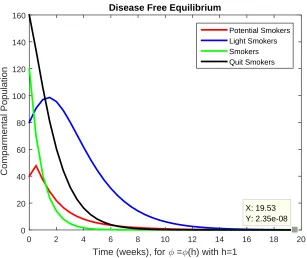
Table 1. Values of physical parameters used in smoking model

Parameter Value Parameter Value

n1 40 n2 40

n3 60 n4 80

n5 200 d1 0.33

d2 0.44 d3 0.55

d4 0.66 β1 0.001

β2 0.001 µ 0.05

b 0.1 γ 0.99

τ 0.2

7. Nonstandard finite difference (NSFD) scheme

A nonstandard finite difference (NSFD) scheme for the system (2.1−2.5) is presented in this section [29].

In recent years, nonstandard finite difference (NSFD) scheme for discrete models have been constructed or

tested for a wide range of nonlinear systems of differential equations [30–32]. The positivity of the state

variables involved in the system is satisfy by proposed method. This property has key role when we solve

mathematical models arising in biology because these state variables represent sub-populations which never

take negative values. The discretized form of the the system (2.1−2.5) by using NSFD scheme which based

on the generalized first order forward method is written as

Pk+1₋_Pk

φ =bN

k₋_β1Lk_Pk+1₋_(d1₊_µ)Pk+1₊_{τ Q}k _(7.1)

Pk+1+β1LkPk+1φ+φ(d1+µ)Pk+1=Pk+bφNk+τ φQk (7.2)

Pk+1= P

k₊_bφNk₊_{τ φQ}k

1 +β1Lkφ+φ(d1+µ)

(7.3)

Lk+1₋_Lk

φ =β1L

k

Pk+1−β2Lk+1Sk−(d2+µ)Lk+1 (7.4)

Lk+1+φβ2Lk+1Sk+φ(d2+µ)Lk+1=Lk+β1LkPk+1 (7.5)

Lk+1= L

k₊_β1Lk_Pk+1

1 +φβ2Sk+φ(d2+µ)

(9)

Sk+1−Sk

φ =β2L

k+1_Sk₋_Sk+1_(γ₊_d3₊_µ) _(7.7)

Sk+1 =β2Lk+1Skφ−φSk+1(γ+d3+µ) (7.8)

Sk+1(1 +φ(γ+d3+µ)) =β2Lk+1Skφ+Sk (7.9)

Sk+1= β2L

k+1_Sk_φ₊_Sk

1 +φ(γ+d3+µ) (7.10)

Qk+1−Qk=φγSk+1−φ(τ+d4+µ)Qk+1 (7.11)

Qk+1(1 +φ(τ+d4+µ)) =φγSk+1+Qk (7.12)

Qk+1= φγS

k+1₊_Qk

1 +φ(τ+d4+µ) (7.13)

which is the purposed NSFD scheme for the given model, where

φ=φ(h) =1−e

−(d3+µ+γ)h

d3+µ+γ (7.14)

The discrete method given in (22,25,29,32) is indeed an NSFD scheme because it is constructed according

to Mickens rules [32] formalized as follows in [33]. Rule 1. The standard denominatorh= ∆tof the discrete

derivatives is replaced by the complex denominator function in Equation (33) which satisfies the asymptotic

relation

φ(h) =h+O(h2)

Note that the denominator function φis expected to better capture the dynamics of the continuous model

through the presence of the underlying parameters d3, µ, γ. In fact, exact schemes for a wide range of

dynamical systems involve such complex denominator functions [34,35]. Rule 2. Nonlinear terms in the

right-hand side of Equation (2.1−2.5) are approximated in a non-local way. For instance, we haveLtkPtk'

LkPk+1 instead ofLtkStk'LkPk

8. _{Analysis of the scheme}

Theorem 5: The NSFD scheme (22,25,29,32) is a dynamical system on the biological feasible domainK

of the continuous model (2.1−2.5).

Proof: First, we prove the positivity of the scheme (22,25,29,32). It is easy to show that the NSFD scheme

(22,25,29,32) takes the explicit form

Pk+1= P

k₊_bφNk₊_{τ φQ}k

(10)

Lk+1= L

k_{(1 +}_β1Lk_φ₊_φ(d1₊_{µ)) + (β1L}k_)(Pk₊_bφNk₊_{τ φQ}k₎

(1 +φβ2Sk+φ(d2+µ))(1 +β1Lkφ+φ(d1+µ))

Sk+1= β2S

k_φA₊_Sk_B

(1 +φ(γ+d3+µ))B

Qk+1=φγ(β2S

k_φA₊_Sk_{B) +}_Qk_{(1 +}_φ(γ₊_d

3+µ))B (1 +φ(τ+d4+µ))(1 +φ(γ+d3+µ))B

where

A=Lk(1+β1Lkφ+φ(d1+µ))+(β1Lk)(Pk+bφNk+τ φQk), B= (1+φβ2Sk+φ(d2+µ))(1+β1Lkφ+φ(d1+µ))

Thus Pk+1 ≥ 0, Lk+1 ≥0, Sk+1 ≥0, Qk+1 ≥0 whenever the discrete variables are non-negative at the

previous iteration. It remains to prove the positive invariance ofK. Adding the (22,25) and (29) we have

[1 +φ(d1+µ)]Hk+1=φbN +Hk−[1 + (d2+µ)φ]Lk+1−[1 +φ(γ+d3+µ)]Sk+1≤φbN+Hk

[1 +φ(µ+d1)]Hk+1≤φbN+Hk

⇒Hk+1≤ bN d1+µ

whenever

Hk≤ bN µ+d1

The priori bonds forQk+1 and Nk+1 follow the radially from the fact thatLk+1 andSk+1 are less then or

equal toHk+1_{. This complete the proof.}

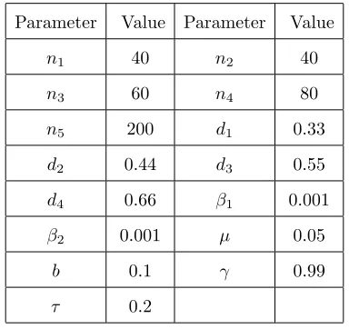
9. Numerical Simulations

The mathematical analysis of smoking epidemic model with non-linear incidence has been presented.

Firstly, we investigate the basic reproduction numberR0for the system (2.1−2.5) which completely

charac-terized the stability of the disease free and endemic equilibrium. We observed that, ifR0<1, the disease free

state atE0andE1is locally stable. To observe the effects of the parameters using in this dynamics smoking

model (2.1−2.5), conclude several numerical simulations varying the value of parameters. These simulations

reveals that a change in time and step sizehaffects the dynamics of the epidemic as shown in Figures 1 and

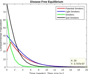
Figures 2. By applying the Mickens approach, we useφ=φ(h) instead of step sizehin figure 2 and figure 4.

comparison is made by highlighting the point in each graph which shows that the Smokers reduces within 20

weeks when we usedφ. Its interpretation for a longer period reduces the infected individuals in the health

system. When initial condition changes to P(0) = 40, L(0) = 80, S(0) = 120, Q(0) = 160, N(0) = 400, the

(11)

Time (weeks), Step size h=1

0 2 4 6 8 10 12 14 16 18 20

Comparmental Population

0 10 20 30 40 50 60 70

80 Disease Free Equilibrium

Potential Smokers Light Smokers Smokers Quit Smokers

X: 20 Y: 3.747e-07

Figure 1. Numerical solutions for potential smokers, Light Smokers, Smokers and Quit

Smokers in a timet(weeks) with step sizeh= 1

Time (weeks),for φ =φ(h) with h=1

0 2 4 6 8 10 12 14 16 18 20

0 10 20 30 40 50 60 70

X: 19.53 Y: 8.774e-09

(12)

Time (weeks), Step size h=1

0 2 4 6 8 10 12 14 16 18 20

0 20 40 60 80 100 120 140

X: 20 Y: 9.083e-07

Smokers in a timet(weeks) with step sizeh= 1 with different initial conditions

Time (weeks), for φ =φ(h) with h=1

0 2 4 6 8 10 12 14 16 18 20

0 20 40 60 80 100 120 140

X: 19.53 Y: 2.35e-08

(13)

10. _Conclusion

It is an important to note that nonstandard finite difference scheme for mathematical models based on

system of differential equations is more powerful approach to compute the convergent solution. The

con-structed unconditionally convergent nonstandard finite difference (NSFD) scheme for smoking model preserve

the positivity of all values ofh(step size) which shows that the developed Scheme is stable. The nonstandard

finite difference scheme is dynamically consistent, easy to implement and shows a good agreement to analyze

the bad impact of smoking for long period of time and represents their dynamical behavior graphically.

Threshold condition shows most sensitive effect regarding their parameters. We prove the essential

proper-ties, bounded, positivity and well-posed, also local and global stability analysis has been made to analyze

the smoking effects in the community. Numerical simulations are carried out to check the actual behavior

of the model.

References

[1] J. Biazar, Solution of the epidemic model by Adomian decomposition method, Appl. Math. Comput. 173 (2006), 1101-1106. [2] S. Busenberg and P. Driessche, Analysis of a disease transmission model in a population with varying size, J. Math. Biol.

28 (1990), 65-82.

[3] A.M.A. El-Sayed, S.Z. Rida and A.A.M. Arafa, On the solutions of time-fractional bacterial chemotaxis in a diffusion gradient chamber, Int. J. Nonlinear Sci. 7 (2009), 485-495.

[4] A.A.M. Arafa, S.Z. Rida and M. Khalil, Fractional modeling dynamics of HIV and 4 T-cells during primary infection, Nonlinear Biomed. Phys. 6 (2012), 1-7.

[5] C.M. Kribs-Zaleta, Structured models for heterosexual disease transmission, Math. Biosci. 160 (1999), 83-108.

[6] B. Buonomo and D. Lacitignola, On the dynamics of an SEIR epidemic model with a convex incidence rate, Ricerche Mat. 57 (2008), 261-281.

[7] X. Liu and C. Wang, Bifurcation of a predator-prey model with disease in the prey, Nonlinear Dyn. 62 (2010), 841-850. [8] F. Haq, K. Shah, G.U Rahman and M. Shahzad. Numerical solution of fractional order smoking model via laplace Adomian

decomposition method, Alex. Eng. J. 57 (2018), 1061-1069.

[9] C. Chavez and B. Song; Dynamical models of tuberculosis and their applications; Math. Biosci. Eng. 1 (2004), 361-404. [10] A. McNeill, M. Raw, J. Whybrow and P. Bailey; National strategy for smoking cessation treatment in England; Addiction

100 (S.2) (2005), 1-11.

[11] R.P. Sargent, R.M. Shepard and S.A. Glantz; Admission for myocardial infarction associated with public smoking bun; Br.Med. J. 1 (2004), 328-977.

[12] Y.M. Terry-McElrath, M.A. Wakefield, S. Emery, H. Saffer, G.M. Szczypka and P. O. Malley P; State antitobacco adver-tising and smoking outcomes by gender and race/ethnicity; Ethnicity and Health 12 (2007), 339-362.

[13] R. Ullah, M. Khan, G. Zaman, S. Islam, M.A. Khan, S. Jan and T. Gul, Dynamical Featurers of mathemtical model on smoking, J. Appl. Environ. Biol. Sci., 6 (2016), 92-96.

(14)

[16] C. Castillo-Garsow, G. Jordan-Salivia, and A. Rodriguez Herrera, Mathematical models for the dynamics of tobacco use, recovery, and relapse, Technical Report Series BU-1505- M, Cornell University, Ithaca, NY, USA,(1997).

[17] O. Sharomi and A. B. Gumel, Curtailing smoking dynamics: A mathematical modeling approach, Appl. Math. Comput. 195 (2008), 475-499.

[18] G. Zaman, Qualitative behavior of giving up smoking model; Bull. Malaysian Math. Sci. Soc. 2 (2011), 403-415. [19] S.A. Matintu, Smoking as Epedemic: Modeling and Simulation study, American J. Appl. Math. 5 (2017), 31-38.

[20] A. Ahmad, M. Farman, F. Yasin and M. O. Ahmad, Dynamical transmission and effect of smoking in society, Int. J. Adv. Appl. Sci. 5(2) (2018), 71-75

[21] F. Ashraf, A. Ahmad, M. U. Saleem, M. Farman and M.O. Ahmad, Dynamical behavior of HIV immunology model with non-integer time fractional derivatives, Int. J. Adv. Appl. Sci. 5(3) (2018), 39-45, .

[22] A. Ahmad, M. Farman, M. O Ahmad, N. Raza and Abdullah, Dynamical behavior of SIR epidemic model with non-integer time fractional derivatives: A mathematical analysis, Int. J. Adv. Appl. Sci. 5(1) (2018), 123-129.

[23] J.B. Swartz, Use of a multistage model to predict time trends in smoking induced lung cancer, J. Epidemiol. Commun. Healt. 46 (1992), 11-31.

[24] F. Brauer and C. Castillo-Cha vez, Mathematical Models in Population Biology and Epidemiology, Springer, (2001). [25] A. Zeb, G. Zaman, V.S. Erturk, B. Alzalg, F. Yousafzai and M. Khan, Approximating a giving up smoking dynamic on

adolescent nicotine dependence in fractional order, PLoS ONE, 11 (2016), 10-15.

[26] G. Zaman, Optimal campaign in the smoking dynamics, Comput. Math. Method. Med. 2011 (2011), Article ID 163834. [27] G. Zaman, Qualitative behavior of giving up smoking models, Bull. Malay. Math. Sci. Soc. 34 (2011), 403-415.

[28] V. Suat Erturk, G. Zamanb and S. Momanic, A numeric analytic method for approximating a giving up smoking model containing fractional derivatives, Comput. Math. Appl. 64 (2012), 3065-3074.

[29] R. E. Mickens, Exact solutions to a finite difference model of a nonlinear reactions advection equation: Implications for numerical analysis, Numer. Methods Partial Differ. Equations, 5 (1989), 313-325.

[30] R. E.Mickens, Applications of Nonstandard finite difference Schemes, World Scientific, Singaporen (2000).

[31] R. Anguelov and J. M.-S. Lubuma, Nonstandard finite difference method by nonlocal approximations, Math. Comput. Simul. 61 (2003), 465-475.

[32] R. E. Mickens, Nonstandard finite difference Models of differential equations, World Scientific, Singapore (1994). [33] R. Anguelov and J.M.-S. Lubuma, Contributions to the mathematics of the nonstandard nite

dierencemethodandapplica-tions, Numer. Methods Partial Differ. Equadierencemethodandapplica-tions, 17 (2001), 518-543.

[34] J.M.-S. Lubuma and K.C. Patidar, Non-standard methods for singularly perturbed problems possessing oscillatory/layer solutions, Appl. Math. Comput. 187(2) (2007), 1147-1160.