ROBOT TRAJECTORY TRACKING WITH ADAPTIVE RBFNN-BASED
FUZZY SLIDING MODE CONTROL
Ayca Gokhan Ak
Vocational School of Technical Sciences Marmara University, Goztepe, Istanbul, Turkey
e-mail: [email protected]
Galip Cansever, Akin Delibasi
Department of Control and Automation Engineering Yildiz Technical University, Besiktas, Istanbul, Turkey
Abstract. Due to computational burden and dynamic uncertainty, the classical model-based control approaches are hard to be implemented in the multivariable robotic systems. In this paper, a model-free fuzzy sliding mode control based on neural network is proposed. In classical sliding mode controllers, system dynamics and system parameters are required to compute the equivalent control. In Radial Basis Function Neural Network (RBFNN) based fuzzy sliding mode control, a RBFNN is developed to mimic the equivalent control law in the Sliding Mode Control (SMC). The weights of the RBFNN are changed for the system state to hit the sliding surface and slide along it with an adaptive algorithm. The initial weights of the RBFNN are set to zero and then tuned online, no supervised learning procedures are needed. In the proposed method, by introducing the fuzzy concept to the sliding mode and fuzzifying the sliding surface, the chattering can be alleviated. The proposed method is implemented on industrial robot (Manutec-r15) and compared with a PID controller. Experimental studies carried out have shown that this approach is a good candidate for trajectory tracking applications of industrial robot.
Keywords: neural network; fuzzy logic; sliding mode control; robot control.
1. Introduction
As robotics systems make their way into standard practice, they have opened the door a wide spectrum of complex applications. Such applications usually demand the robots to be highly intelligent. In order to provide a high-quality control and performance in ro-botics, new intelligent control techniques must be developed. Hence, the pursuit of intelligent robotics systems has been a topic of much fascinating research in recent years.
On the other hand, as emerging technologies, soft computing paradigms consisting of complementary elements of fuzzy logic and neural network are viewed as the most promising methods towards intelligent ro-botics systems [1].
Sliding Mode Control (SMC), based on the theory of variable structure systems, has attracted a lot of research on control systems for the last two decades. This control scheme suffers from some problems, however. In order to guarantee the stability of the sliding mode system, the boundary of the uncertainty
has to be estimated. A large value has to be applied to the control gain when the boundary is unknown. But, this large control gain may cause chattering on the sliding surface and therefore deteriorate the system performance [2]. Control input may be fuzzified to solve this problem.
In recent years, fuzzy logic in control design has been widely used for numerous electrical systems, ro-botic systems and mechanical systems. The prominent advantage of the fuzzy controller is that it can effec-tively control complex ill-defined systems having non-linearities, parameter variations and disturbances [3].
The second disadvantage of the SMC is the diffi-culty in the calculation of the equivalent computation. A thorough knowledge of the plant dynamics is required for this purpose [4]. The equivalent control has a role similar to the inverse dynamics. An estima-tion technique can be used to compute the equivalent control [5]. Neural networks, especially multilayered perceptron, are the popular tool to compute the equi-valent control [6], [7].
Choi and Kim designed a fuzzy-sliding mode cont-roller by fuzzifiying the sliding surfaces in order to attenuate the chattering [3]. Derbel and Alimi realized a hybrid sliding-and-fuzzy logic controller by fuzzy logic without the computation of the equivalent cont-rol [8]. Ertugrul and Kaynak utilized two parallel neu-ral networks to realize a neuro-SMC. In their work, equivalent control and corrective control terms of SMC are the outputs of the two layer feed-forward neural networks [7]. Abdelhameed used chattering index to tune adaptively the switching gain of the sliding mode controller in order to shorten the du-ration of reaching phase and to minimize chattering of the control action of SMC [9]. Hussain and Ho incorporated both prior knowledge and neural networks in the SMC with boundary layer approach [10]. Javaheri and Vossoughi designed a fuzzy cont-roller to enhance the performance. Contcont-roller conti-nuously optimizes the sliding mode parameters inclu-ding hitting control gain, boundary layer thickness, sliding surface slope and intercept [11]. A discussion on how some “intelligence” can be incorporated in SMCs by the use of computational intelligence metho-dologies and an overview of the research and appli-cations reported in the literature in this respect is presented in Kaynak et al. paper [12].
In this paper, a synergistic combination of Radial Basis Function Neural Network (RBFNN) with fuzzy sliding mode control methodology is proposed. The slope of the sliding surface is used to adjust with Fuzzy logic. The weights of the RBFNN are adjusted according to an adaptive algorithm for the purpose of controlling the system states to hit the sliding surface and then slide along it. The proposed method and PID control are implemented on an industrial robot (Manu-tec-r15) and the results obtained from the applications are presented.
The paper is organized as follows: In Section 2, adaptive RBFNN-based fuzzy sliding mode control design is presented. Experimental setup is explained in Section 3. Results are presented in Section 4. Section 5 concludes the paper.
2. Design of the control system
2.1. Sliding Mode Control
Variable Structure System (VSC) and SMC that is a special kind of VSC are widely used in robotics. The basic idea is to alter the system dynamics some sur-faces in the state space so that the states of the system are attracted to these surfaces. During the sliding mo-tion of the state on the surface, the system remains insensitive to parameter deviation and external distur-bances.
The dynamic model of the robot is the following:
( ) ( , ) ( )
uM q q c q q g q , (1)
where are the joint position, velocity, and
acceleration vectors, respectively;
de-notes the inertia matrix; expresses the
coriolis and centrifugal torques, is the
gra-vity vector; is the actuator torque vector
act-ing on the joints.
n R q q q,,
nxn
R q
M( )
nxn R q q c( ,)
q g( )
1
n R
1 nx
R
u
After transformations x q and x2 q are done,
robot dynamic will take the form Mx C
1
1 0
x g u
2 x2 g x1 M x
. The state space mathematical model of the robot is obtained as follows:
1 1
1 1,
x C x
( , )
1 2 x
u
x M x x
. (2)
Then, the closed form of the robot dynamic is written as follows:
( )
x t f x t Bu, (3)
where B is the input gain matrix.
Sliding surface for system (3) can be chosen as follows:
: ( , )s x t ( )
s x t s xa( )0 , (4)
where ( )t Gx td( ) is the time independent part of
the sliding function, s xa( )Gx t( ) is the state
independent part of the sliding function and is the
target state (reference). Sliding surface variable is in the following form
d
x
1
i
k
i i
d
i
s e
dt
, (5)
where e is the error (exdx ) and i is a positive constant defined by designer.
In a robotic system, the purpose of the control is to provide tracking ofq t( )q td( ) trajectory by robot. In this situation, simple and general selection of sliding mode surface is s0 for 0[13].
The control should be chosen in such a way that the candidate Lyapunov function would satisfy Lyapunov criteria. The Lyapunov function (positive definite) is selected as follows:
( ) 2
T
s s
V s . (6)
It is aimed that the derivative of the Lyapunov function would be negative definite. This can be guaranteed if one can assure that
( )
( )
T
dV s
s Dsig
(
T T
n s
dt , (7)
where D is a positive definite diagonal matrix.
Taking the derivative of (6), equating (7) and using system equation we obtain
)
s s s Dsign s . (8)
,a
s
s x G f x t Bu t
x
. (9)
If expression (8) is replaced with (9), sliding mode control law can be represented as:
eq c
u
u
u
, (10)where is the equivalent control law for sliding
phase motion and is the corrective control for the
reaching phase motion. The control objective is to guarantee that the state trajectory can converge to the
sliding surface. So, corrective control is chosen as
follows: eq u
c
u
c
u
( )
c sign s
u K , (11)
where K is a positive constant. The controller in (10)
results with high frequency oscillations, defined as
chattering. The function is a discontinuous
function:
sign
1 0
( ) 0 0
1 0
s
sign s s
s
. (12)
2.2. Adaptive RBFN-based fuzzy sliding mode control
The control law for the proposed controller is as
(9) form. The slope of the sliding surface () is
adjusted with fuzzy logic and the equivalent control is computed by RBFNN.
eq
u
Absolute error is the input and is the output of
the fuzzy system. The rules in the rule base are as follows:
IF ei is vs, THEN i is xxl IF ei is s, THEN i is xl
IF ei is m, THEN i is l IF ei is l, THEN i is m
IF ei is xl, THEN i is s IF ei is xxl, THEN
i is vsIt is chosen that both ei and i have the same
kind of membership functions: vs, s, m, l, xl, xxl. The input and output membership functions are of the same structure (Figure 1).
Figure 1. Input and output membership functions
From the knowledge of the fuzzy systems, i can
be written as;
( )
T i ki ki ei
, (13)
where ki
ki1,,...,kim,...,kiMr
T is the vector of thecenter of the membership functions of i,
Ti i
ki(e (e )
M
ki i m ki i 1
ki(e ),..., (e ),... r
) is the vector
of the height of the membership functions of i in
which , and is
the amount of the rules.
r
m
M
1 m i A i m
ki(e ) (e )/
Am( )ei Mr
A RBFNN is employed to model the relationship between the sliding surface variable, s, and equivalent
control, . In other words, sliding variable s will be
used as the input signal for establishing a RBFNN mo-del to calculate the equivalent control [2].
eq
u
The architecture of RBFNN is shown in Figure 2. The network consists of three layers: an input layer, a single layer of nonlinear processing neurons, and an output layer. The output of the RBFNN is calculated according to
1 1
( , )
N N
eq ij j j ij j j
j j
u w x c w x c
m
1, 2,...,
i , (14)
where xnx1 is an input vector, is a function
from
.j
(set of all positive real numbers) to , . is
the Euclidean norm, are the weights in the output
layer, N is the number of neurons in the hidden layer,
and
ij
w
1
nx j
c are the RBF centers in the input vector
space. For each neuron in the hidden layer, the Euc-lidean distance between its associated center and the input to the network is computed. The output of the neuron in a hidden layer is a nonlinear function of the distance. Finally, the output of the network is com-puted as a weighted sum of the hidden layer outputs [14]. Most preferred is the Gaussian function:
2
2( ) exp j
j
j
s c
s
. (15)
Based on the Lyapunov theorem, the condition of
reaching the sliding surface is . If the control
input chooses to satisfy this reaching condition, the control system will converge to the origin of the phase plane. Since a RBFNN is used to approximate the non-linear mapping between the sliding variable and the control law, the weights of the RBFNN should be adjusted based on the reaching condition.
0
s
s
Figure 2. Radial Basis Function Neural Network (RBFNN)
The adaptive rule is derived from the steepest
descent rule to minimize the value of with respect
to . Then the updated equation of the weight
para-meters is [15]:
s
s
j
w
( ) ( ) ( )
j
j
s t s t w
w t
, (16)
where is adaptive rate parameter. Using the chain
rule, (16) can be rewritten as follows:
2
( ) ( )
( ) ( )
( )
( ) ( )
( ) exp ( ) ( )
eq eq j
eq j
j
j j
u t u t
s t s t
w B
u t w t t
s c
s t
s t s
t s
, (17)
where and system parameter are combined as a
learning parameter,.
3. Experimental Setup
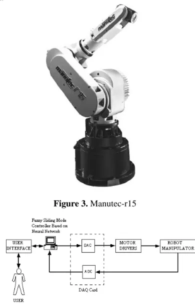
The robot manipulator used in experiments is Manutec-r15 with 6 degree of freedom (Figure 3). Ro-bot has 3 phase, brushless synchronous motors. RoRo-bot has incremental encoders (axis 1:600, axis 2: 1200, axis 3: 600, axis 4: 360, axis 5: 320, axis 6: 500). The malfunctioned original control and driver unit of the Manutec-r15 were deactivated and a new transformer, a new driver system, a new control system was built up to try the control methods on the robot.
The block diagram of the system is shown in Figure 4. A circuit is designed to isolate the digital in-put-output. Simple filters are emplaced to eliminate wrong measures because of cable length that connect the systems. Experiments were executed at three axis of the robot. DAQ Card is 16 Bits, 299kS/s and has 8 Digital I/O, 2 Analog output 2, 24 bit counter/timers.
Features of the computer used on the system are Pentium 4, CPU 3.2 GHz and 512 MB RAM.
Robot was controlled with data obtained from DAQ card through Wincon software on Matlab Simu-link.
Figure 3. Manutec-r15
Figure 4. Block diagram of the system
4. Experimental Results
Experiments are realized on base three axes of the robot but only results of two axes are presented here. After the robot was activated, target trajectory (from
the software) was given is in 6.2th second for axis 1,
12.5th second for axis 2. System was closed about 48th
for axis 1 and 65th second for axis 2. Desired and
ac-tual states positions of two axes are shown in Fig 5. Desired and actual positions are closely near to each other.
The System was also tested with classical PID controller. After the brake is off, the target is switched
on about 15th second for all axes. The system was
closed about 65th second. Desired and actual state
positions of two axes for classical PID method are shown in Figure 6.
0 5 10 15 20 25 30 35 40 45 50 -15
-10 -5 0 5 10 15
Time(s)
P
o
s
it
io
n1(Deg
ree)
Actual Position Desired Position
(a)
0 10 20 30 40 50 60 70
150 152 154 156 158 160 162 164
Time (s)
P
o
s
it
io
n2(Deg
ree)
Actual Position Desired Position
(b)
Figure 5. Desired and actual states positions of two axes for adaptive RBFNN-based fuzzy sliding mode control
(a) for axis 1 and (b) for axis 2
0 10 20 30 40 50 60 70
-15 -10 -5 0 5 10
Time(s)
P
os
it
ion
1(
Degr
e
e)
Actual Position Desired Position
(a)
0 10 20 30 40 50 60 70 152
154 156 158 160 162
Time(s)
P
os
it
io
n2(
D
egr
ee
)
Actual Position Desired Position
(b)
Figure 6. Desired and actual states positions of two axes for PID control (a) for axis 1 and (b) for axis 2
0 10 20 30 40 50 60 70
-2 0 2 4 6 8 10
Time(s)
E
rro
r1
(De
g
re
e
)
Proposed Control PID Control
0 10 20 30 40 50 60 70
-1 0 1 2 3
Time(s)
E
rro
r2
(D
e
g
re
e
)
Proposed Control PID Control
(b)
Figure 7. Position errors for two axes for adaptive RBFNN based fuzzy sliding mode control and PID control
(a) for axis 1 and (b) for axis 2
0 10 20 30 40 50 60 70
-1.5 -1 -0.5 0 0.5 1 1.5
Time (s)
u1
(N
m
)
Proposed Control PID Control
(a)
0 10 20 30 40 50 60 70 -2
-1 0 1 2 3
Time(s)
u2(
N
m
)
Proposed Control PID Control
(b)
Figure 8. Control Torque Inputs for two axes adaptive RBFNN based fuzzy sliding mode control and
PID control (a) for axis 1 and (b) for axis 2
5. Conclusions
Adaptive RBFNN-based fuzzy sliding mode cont-rol and application results of the proposed method to the industrial robot are presented in this paper.
Using adaptive RBFNN-based fuzzy sliding mode control, whole knowledge of the system dynamics and system parameters aren’t required to compute the equivalent control. An adaptive rule is utilized for on-line adjusting the weights of RBFNN, which is used to compute the equivalent control. Adaptive training algorithm was derived in the sense of Lyapunov stabi-lity analysis, so the stabistabi-lity of the closed-loop system can be guaranteed. Using fuzzy controller to adjust the slope of the sliding surface control gain in SMC re-duces the reaching time and chattering with respect to classical SMC.
(a)
trajectory. Tracking errors of the proposed controller are smaller than those of classical control. Experi-mental results demonstrate that the adaptive RBFNN-based fuzzy sliding mode control is applicable control scheme for trajectory tracking applications of robotic manipulators.
Acknowledgment
This research has been supported by Yildiz Techni-cal University Scientific Research Projects Coordina-tion Department. Project number: 25-04-02-03.
References
[1] D. Katic, M. Vukobratovic. Intelligent Control of Robotic Systems. Kluwer Academic Publishers, Lon-don, 2003.
[2] Y. Guo, P. Woo. An Adaptive Fuzzy Sliding Mode Controller for Robotic Manipulators. IEEE Transac-tions on Systems, Man, and Cybernetics-Part A: Systems and Humans, Vol.33, No.2, 2003, 149-159. [3] S.B. Choi, J. Kim. A Fuzzy–Sliding Mode Controller
for Robust Tracking of Robotic Manipulators. Mecha-tronics, Vol.7 No.2, 1997, 199-216.
[4] M. Ertugrul, O. Kaynak. Neural Computation of the Equivalent Control in Sliding Mode for Robot Trajec-tory Control Applications. IEEE International Confe-rence on Robotics&Automation, 1998, 2042-2047. [5] V. Mkrttchian, A. Lazaryan. Application of Neural
Network in Sliding Mode Control. IEEE International Conference on Control Applications, 2000, 653 – 657. [6] C. Tsai, H. Chung, F. Yu. Neuro-Sliding Mode
Control with Its Applications to Seesaw Systems. IEEE Trans. on Neural Networks, Vol.15, No.1, 2004, 124-134.
[7] M. Ertugrul and O. Kaynak. Neuro Sliding Mode Control of Robotic Manipulators. Mechatronics 10, 2000, 239-263.
[8] N. Derbel, A.M. Alimi. Design of a Fuzzy Sliding mode Controller by Fuzzy Logic. International Jour-nal of Robotics and Automation, Vol. 21, No. 4, 2006, 359-367.
[9] M. Abdelhameed. Adaptive Neural Network Based Controller for Robots. Mechatronics, 1999, 147-162. [10] M. A. Hussain, P.Y. Ho. Adaptive Sliding Mode
Control with Neural Network Based Hybrid Models. Journal of Process Control 14, 2004, 157-176.
[11] H. Javaheri and G.R. Vossoughi. Sliding Mode Control with Online Fuzzy Tuning: Application to a Robot Manipulator. Proceeding of the IEEE Interna-tional Conference on Mechatronics & Automation Ca-nada, 2005, 1357-1362.
[12] O. Kaynak, K. Erbatur, M. Ertugrul. The Fusion of Computationally Intelligent Methodologies and Sli-ding-Mode Control—A Survey. IEEE Trans. Ind. Electronics, Vol.48, 2001, 4- 7.
[13] B. W. Bekit, J.F. Whidborne, L.D. Seneviratne. Fuzzy sliding mode control for a robot manipulator. Computational Intelligence in Robotics and Automation, 1997, 320-325.
[14] F.M. Ham, I. Kostanic. Neurocomputing for Science &Engineering. Mc Graw-Hill Inc., 2001.