Change Point Estimation in Panel Data without
Boundary Issue
Barbora Peštová1,:and Michal Pešta2,:,*
1 Department of Medical Informatics and Biostatistics, Institute of Computer Science, The Czech Academy of Sciences, 117 20 Praha 1-Staré Mˇesto, Czech Republic; [email protected]
2 Department of Probability and Mathematical Statistics, Faculty of Mathematics and Physics, Charles University, 116 36 Praha 1-Staré Mˇesto, Czech Republic
* Correspondence: [email protected]; Tel.: +420-608-427-147
: These authors contributed equally to this work.
Abstract: Panel data of our interest consist of a moderate number of panels, while the panels contain a small number of observations. An estimator of common breaks in panel means without a boundary issue for this kind of scenario is proposed. In particular, the novel estimator is able to detect a common break point even when the change happens immediately after the first time point or just before the last observation period. Another advantage of the elaborated change point estimator is that it results in the last observation in situations with no structural breaks. The consistency of the change point estimator in panel data is established. The results are illustrated through a simulation study. As a by-product of the developed estimation technique, a theoretical utilization for correlation structure estimation, hypothesis testing, and bootstrapping in panel data is demonstrated. A practical application to non-life insurance is presented as well.
Keywords: change point; estimation; consistency; panel data; short panels; boundary issue; structural change; bootstrap; non-life insurance; change in claim amounts
MSC:62F10, 62F40, 62H12, 62H15, 62E20, 62P05
JEL:C330, C130, C120, C150, G220
1. Introduction and Main Aims
The problem of an unknown common change in means of the panels is studied, where the panel data consist of Npanels and each panel contains T observations over time. Various values of the change are possible for each panel at some unknown common time τ “ 1, . . . ,T. The panels are considered to be independent, although this restriction can be weakened. On the other hand, within the panels, the observations are generally not assumed to be independent. This is in accordance with typical assumptions that one can make about real data. A common dependence structure is supposed to be present over the panels. Our main goal is to construct anestimatorof a possible change point, which isconsistenteven in case of no structural break.
1.1. Current State of Art
point estimator was introduced, requiring no definite knowledge about existence of the change point in the given panel data. In the case of no change being present, the estimator picks the last observation, which means that no structural break is identified. However, this estimator has several disadvantages. It assumes a certain kind of homoscedasticity in the panels. Further, it does not take into account the possibility that the change may occur right after the first time point. It also assumes conditions that may be viewed as too complicated with regard to verification and model checking. The remaining task is, therefore, to develop a change point estimator that is consistent regardless of the change’s presence/absence. Moreover, such estimator would gain from allowingheteroscedasticity in the panels, having broader scope of applications. Besides that, the applicability of the estimator is enhanced by simple consistency conditions and noboundary issue. The boundary issue means that the change point can neither be detected nor estimated when being close to the beginning or to the end of the observation regime.
Further on, [5] and [6] dealt with the change point estimator under cross sectional dependence in the panels modeled by a common factor, and expanded the estimation problem for more complicated types of structural changes. The first and second order asymptotics that can be used to derive consistent confidence intervals for the time of change in panel data was established by [7]. The panel lengthTwas considered as unbounded and depending on the number of panelsN. However, there is some literature on the short panel change point framework where also weighting functions, as we employ later on, are suggested, cf. [8].
1.2. Motivation in Non-life Insurance
Structural changes in panel data—especially common breaks in means—are wide spread phenomena. Our primary motivation comes from non-life insurance business, where associations in many countries uniting several insurance companies collect claim amounts paid by every insurance company each year. Such a database of cumulative claim payments can be viewed as panel data, where insurance companyi“1, . . . ,Nprovides the total claim amountYi,tpaid in yeart“1, . . . ,T into the common database. The members of the association can consequently profit from the joint database.
For the whole association it is important to know, whether a possible change in the claim amounts occurred during the observed time horizon. Usually, the time period is relatively short, e.g., 10–15 years. To be more specific, a widely used and very standard actuarial method for predicting future claim amounts—called chain ladder—assumes a kind of stability of the historical claim amounts. The formal necessary and sufficient condition is derived in [9]. This paper shows a way how to detect a possible historical instability.
1.3. Structure of the Paper
The remainder of the paper is organized as follows. Section2introduces an abrupt change point model together with stochastic assumptions. An estimator for the change point in panel means is proposed in Section 3. Consequently, consistency of the considered change point estimator is derived, which covers the first main theoretical contribution. Section4contains a simulation study that illustrates finite sample performance of the estimator. It numerically emphasizes the advantages and disadvantages of the proposed approach. The second main theoretical contribution lies in the panel correlation structure estimation and in the bootstrap add-on justification for hypothesis testing, all provided in Section5. A practical application of the developed approach to an actuarial problem is presented in Section6. Proofs are given in the Appendix.
2. Abrupt Change in Panel Data
Let us consider the panel change point model
whereσi ą0 are unknown variance-scaling panel-specific parameters andTis fixed, not depending onN. The possiblecommon change point timeis denoted byτP t1, . . . ,Tu. A situation whereτ “T corresponds tono changein means of the panels. The meansµiare panel-individual. The amount of the break in mean, which can also differ for every panel, is denoted byδi. There is at most one change per panel in model (1) and the type of change in the panel mean isabrupt.
Furthermore, it is assumed that the sequences of panel disturbances tεi,tut are independent. At the same time, the errors within each panel form a weakly stationary sequence with a common correlation structure. This can be formalized in the following assumption.
Assumption A1. The vectorsrεi,1, . . . ,εi,TsJ existing on a probability spacepΩ,F,Pqareiidfori “ 1, . . . ,NwithEεi,t“0 andVarεi,t“1, having the autocorrelation function
ρt“Corr`εi,s,εi,s`t
˘
“Cov`εi,s,εi,s`t
˘
, @sP t1, . . . ,T´tu, which is independent of the lags, the cumulative autocorrelation function
rptq “Var
t
ÿ
s“1 εi,s“
ÿ
|s|ăt
pt´ |s|qρs,
and the shifted cumulative correlation function
Rpt,vq “Cov
˜ t ÿ
s“1 εi,s,
v
ÿ
u“t`1 εi,u
¸
“ t
ÿ
s“1 v
ÿ
u“t`1
ρu´s, tăv
for alli “1, . . . ,Nandt,v “1, . . . ,T. The covariance matrixΛ:“Var ”ř1
s“1ε1,s, . . . ,
řT s“1ε1,s
ıJ is non-singular.
The sequencetεi,tuTt“1 can be viewed as a part of a weakly stationary process. Note that the within-panel dependent errors do not necessarily need to be linear processes. GARCH processes are a plausible alternative, for instance.
The assumption of independent panels can be relaxed. It would, however, make the setup much more complex, cf. [5]. Consequently, probabilistic tools for dependent data need to be used (e.g., suitable versions of the central limit theorem). Nevertheless, assuming, that the claim amounts for different insurance companies are independent, is reasonable with regard to real life experience.
Assumption A2. There exist constantsσ,σą0 not depending onN, such that σďσi ďσ, 1ďiďN.
The assumption of the bounded panel variances from both below and above allows for heteroscedasticity between the panels. In case, when the equiboundedness cannot be satisfied, the panel model can be generalized by introducing weights wi,t, which are supposed to be known. Subsequently, claim ratiosYi,t{wi,t can be modeled. Being particular in actuarial practice, it would mean to normalize the total claim amount by the premium received (considered as the weight), since bigger insurance companies are expected to have higher variability in total claim amounts paid.
3. Change Point Estimator
to one. In other words, the value of the change point estimate can beTmeaning no change. This is in contrast to [3], whereTis not reachable.
Our estimator of the time of changeτin panel data is defined as
p
τN:“arg min t“1,...,T
N
ÿ
i“1
#
1 wptq
t
ÿ
s“1
pYi,s´Ysi,tq2`
1 wpT´tq
T
ÿ
s“t`1
pYi,s´Yri,tq2 +
, (2)
whereYsi,tis the average of the firsttobservations in paneliandYri,tis the average of the lastT´t
observations in paneli, i.e.,
s
Yi,t“ 1
t t
ÿ
s“1
Yi,s and Yri,t“
1 T´t
T
ÿ
s“t`1 Yi,s.
By convention, the value of an empty sum is zero. A sequence of positive weights twptquTt“0 is specified later on.
3.1. Consistency
We postulate additional assumptions on the panel change point model (1) in order to derive the estimator’s consistency. The following conditions take into account that the length T of the observation regime is fixed; that the lengthTdoes not depend on the number of panelsN; and that the lengthTcan even be relatively small.
Assumption A3. Let gptq:“ wpttq
´
1´rpt2tq
¯
for tP t1, . . . ,Tu, gp0q ”0, and
lim NÑ8
1 ?
N
#
τ τ`1
N
ÿ
i“1
δi2´ pgpτq `gpT´τqq max t“1,...,Twptq
N
ÿ
i“1 σi2
+
“ 8,
lim NÑ8
1 ?
N
#
T´τ T´τ`1
N
ÿ
i“1
δi2´ pgpτq `gpT´τqq max t“1,...,Twptq
N
ÿ
i“1 σi2
+
“ 8.
Assumption A4. limNÑ8 N12
řN
i“1δ2i “0. Assumption A5. Eε41,tă 8,tP t1, . . . ,Tu.
Theorem 1(Change point estimator consistency). Under AssumptionsA1–A5 lim
NÑ8PrpτN“τs “1.
The formally postulated estimator’s consistency in Theorem1can be practically interpreted: as one observes more and more panels, the probability that the proposed estimator is different from the true unknown change point gets smaller and smaller.
AssumptionA3 is not restrictive at all, although it may be seen as a complicated one. For example in case of independent observations within the panel (i.e.,rptq “t) and the weight function wptq “ tq,q ě 2 fort P t1, . . . ,Tu,wp0q “1, the sequencetgptqutT“2becomestt1´q´t´quT
t“2and is non-increasing. Then AssumptionA3is automatically fulfilled, ifq“2 and ?1
N
řN i“1
`
AssumptionsA3andA4are satisfied, for instance, if 0ăδďδiď∆for alli’s (a common lower and upper threshold for the means’ shifts),δ2 “O`Nζ˘,ζ ą0 and∆2{N Ñ 0 asN Ñ 8(bearing in mind AssumptionA2). Another suitable example of δi’s for the conditions in Assumptions A3 andA4, can be δi “ Kiη for someK ą 0 and 0 ă η ă 1{2. ConditionsA3and A4do not require each panel to have a break. Sometimes, a more restrictive assumption can be assumed instead of AssumptionsA3andA4, e.g.,
lim NÑ8
1 N
N
ÿ
i“1
δ2i “ 8. (3)
On one hand, this assumption might be considered as too strong, because a common fixed (not depending on N) value of δ “ δi for alli’s does not fulfill (3). On the other hand, (3) is satisfied whenδ2j{N Ñ 8 as N Ñ 8 for some j P N and δi “ 0 for all i ‰ j. This stands for a situation when all the panels do not change in mean except one panel having a sufficiently large change in mean with respect to the number of panels. Let us notice that one could replace AssumptionA3with a stronger assumption from (3), but it would mean disappearing the detectability relation between the size of breaks and the variability of errors. One would also lose an idea how to choose the weights. Furthermore, Assumptions E1 and E2 from [4] are more restrictive than AssumptionA3, which makes the presented approach even more general.
Various competing consistent estimators of a possible change point can be suggested, e.g., the
maximizer ofřN i“1
” řt
s“1pYi,s´tYsi,Tq ı2
as in [7]. To show consistency of this estimator, one needs to postulate different assumptions on the cumulative autocorrelation function and this may be rather complex.
In our opinion, it is erroneously assumed in [3] that only the second moment of the errors is sufficient to prove the consistency result. In particular, Lemma A.1 from [3] has to require the finite fourth errors’ moments, which coincides with AssumptionA5.
4. Simulation Study
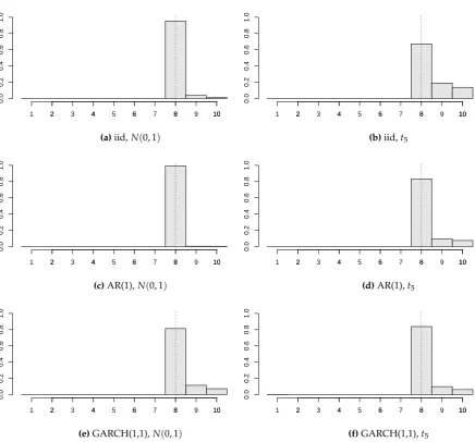
A simulation experiment was performed to study thefinite sampleproperties of the change point estimator for a common abrupt change in panel means. In particular, the interest lies in theempirical distributions of the proposed estimator visualized via histograms. Random samples of panel data (2000 each time) are generated from the panel change point model (1). The panel size is set toT“10 in order to demonstrate the performance of the estimator in case of small panel length. The number of panels considered isN“2, 5, 10, 20, 50.
The correlation structure within each panel is modeled via random vectors generated from iid, AR(1), and GARCH(1,1) sequences. The considered AR(1) process has coefficientφ “ 0.3. In case of GARCH(1,1) process, we use coefficients α0 “ 1, α1 “ 0.1, and β1 “ 0.2, which according to [10, Example 1] gives a strictly stationary process. In all three sequences, the innovations are obtained as iid random variables from a standard normalNp0, 1qor Studentt5distribution multiplied by a suitable constant in order that the errors possess unit variance (see Assumption A1). The variance-scaling parameters are kept constant for all panels, i.e., σi “ σ for all i. The sequence of weights is chosen astwptq “ t2u10t“1andwp0q “ 1. Monte Carlo simulation scenarios are produced as all possible combinations of the above mentioned settings and a selection of the results is listed below.
Firstly, we examine the impact of the errors’ distribution and the correlation structure on the change point estimator. Figure1contains six different structures of model disturbances, whereτ“8 (depicted by the dotted vertical line),N“20,σ“.2, and all of the panels are subject to break of value δi„Ur0, 2s(i.e., the breaks are independently and uniformly distributed onr0, 2s).
2 4 6 8 10
0.0
0.2
0.4
0.6
0.8
1.0
1 2 3 4 5 6 7 8 9 10
(a)iid,Np0, 1q
2 4 6 8 10
0.0
0.2
0.4
0.6
0.8
1.0
1 2 3 4 5 6 7 8 9 10
(b)iid,t5
2 4 6 8 10
0.0
0.2
0.4
0.6
0.8
1.0
1 2 3 4 5 6 7 8 9 10
(c)AR(1),Np0, 1q
2 4 6 8 10
0.0
0.2
0.4
0.6
0.8
1.0
1 2 3 4 5 6 7 8 9 10
(d)AR(1),t5
2 4 6 8 10
0.0
0.2
0.4
0.6
0.8
1.0
1 2 3 4 5 6 7 8 9 10
(e)GARCH(1,1),Np0, 1q
2 4 6 8 10
0.0
0.2
0.4
0.6
0.8
1.0
1 2 3 4 5 6 7 8 9 10
(f)GARCH(1,1),t5
Figure 1. Histograms of the estimated change pointsτpN for various structures and distributions of the panel disturbances (τ “8,T“10,N “20,σ“.2, all of the panels are subject to break of size δi„Ur0, 2s).
Subfigures1a, 1c, 1e versus Subfigures1b, 1d, 1f). One may notice that the AR(1) errors’ model gives the best estimator’s precision from three correlation structures. This should not be considered as a surprise, because our chosen AR(1) model has a positive autoregression coefficient (φ “ 0.3) and, therefore, the values of gpτq and gpT´τq from Assumption A3 are larger than the values corresponding to the iid errors’ structure. Hence, one can say that the detectability AssumptionA3is satisfied more easily. Loosely speaking, the stronger positive correlations within the panel, the more “deterministic behavior” of the random noise, and the better estimator’s precision.
Figure2demonstrates that the proposed estimator works reasonably for various locations of the unknown change point. Particularly, six values of the common change point (again depicted by the dotted vertical line) are chosen (τ“1, 2, 5, 8, 9, 10) withN“20,σ“.2, 75% of the panels have a break δi„Ur0, 2s, and the panel disturbances come from AR(1) withNp0, 1qinnovations. Recall thatτ“10 corresponds to the ‘no change’ situation and the empirical distribution of the estimator concentrates mainly at the last time point, which is in coherence with the change point formulation from (1).
2 4 6 8 10
0.0
0.2
0.4
0.6
0.8
1.0
1 2 3 4 5 6 7 8 9 10
(a)τ“1
2 4 6 8 10
0.0
0.2
0.4
0.6
0.8
1.0
1 2 3 4 5 6 7 8 9 10
(b)τ“2
2 4 6 8 10
0.0
0.2
0.4
0.6
0.8
1.0
1 2 3 4 5 6 7 8 9 10
(c)τ“5
2 4 6 8 10
0.0
0.2
0.4
0.6
0.8
1.0
1 2 3 4 5 6 7 8 9 10
(d)τ“8
2 4 6 8 10
0.0
0.2
0.4
0.6
0.8
1.0
1 2 3 4 5 6 7 8 9 10
(e)τ“9
2 4 6 8 10
0.0
0.2
0.4
0.6
0.8
1.0
1 2 3 4 5 6 7 8 9 10
(f)τ“10
Figure 2. Histograms of the estimated change pointsτpN for various values of the change point τ (T“10,N“20,σ“.2, 75% of the panels are subject to break of sizeδi„Ur0, 2s, panel disturbances from AR(1) withNp0, 1qinnovations).
innovations. It is clear that the precision ofτpNimproves markedly asNincreases. A higher number of
panels, i.e.,N“50, were also taken into account and, then, 100% precision was achieved. Moreover, longer panels were also simulated (e.g.,T“25), but these results are not presented here. This is due to a simple reason that the precision of the estimator increases as the panel size gets bigger, which is straightforward and expected.
Figure 4 shows the effect of panel variability on the estimator’s performance. In particular, various values of the variance-scaling parameter are considered (σ “ .1, .2, .5, 1.0), where τ “ 1, N“10, all of the panels have a breakδi„Ur0, 2s, and the panel disturbances come from GARCH(1,1) withNp0, 1qinnovations. It can be seen that the less volatile observations, the more precise change point estimate. The panel’s variability under the considered dependency can be too high compared to the change size. Then, it would be rather difficult to detect a possible change as for instance in Subfigure4dthat corresponds toσ“1.0.
2 4 6 8 10
0.0
0.2
0.4
0.6
0.8
1.0
1 2 3 4 5 6 7 8 9 10
(a)N“2
2 4 6 8 10
0.0
0.2
0.4
0.6
0.8
1.0
1 2 3 4 5 6 7 8 9 10
(b)N“5
2 4 6 8 10
0.0
0.2
0.4
0.6
0.8
1.0
1 2 3 4 5 6 7 8 9 10
(c)N“10
2 4 6 8 10
0.0
0.2
0.4
0.6
0.8
1.0
1 2 3 4 5 6 7 8 9 10
(d)N“20
Figure 3. Histograms of the estimated change pointspτN for various values of N (τ “ 9, T “ 10, σ“.2, 50% of the panels are subject to break of sizeδi„Ur0, 2s, panel disturbances from AR(1) with t5innovations).
2 4 6 8 10
0.0
0.2
0.4
0.6
0.8
1.0
1 2 3 4 5 6 7 8 9 10
(a)σ“.1
2 4 6 8 10
0.0
0.2
0.4
0.6
0.8
1.0
1 2 3 4 5 6 7 8 9 10
(b)σ“.2
2 4 6 8 10
0.0
0.2
0.4
0.6
0.8
1.0
1 2 3 4 5 6 7 8 9 10
(c)σ“.5
2 4 6 8 10
0.0
0.2
0.4
0.6
0.8
1.0
1 2 3 4 5 6 7 8 9 10
(d)σ“1.0
innovations. One can conclude that higher precision is obtained when a larger portion of panels is subject to change in mean. If a small number of panels contain a break (for example Subfigure5a), then the change point estimator does not perform well.
2 4 6 8 10
0.0
0.2
0.4
0.6
0.8
1.0
1 2 3 4 5 6 7 8 9 10
(a)25%
2 4 6 8 10
0.0
0.2
0.4
0.6
0.8
1.0
1 2 3 4 5 6 7 8 9 10
(b)50%
2 4 6 8 10
0.0
0.2
0.4
0.6
0.8
1.0
1 2 3 4 5 6 7 8 9 10
(c)75%
2 4 6 8 10
0.0
0.2
0.4
0.6
0.8
1.0
1 2 3 4 5 6 7 8 9 10
(d)100%
Figure 5.Histograms of the estimated change pointsτNp when various portion of the panels are subject to break of sizeδi „Ur0, 2s(τ “5,T “10,N “20, panel disturbances from GARCH(1,1) witht5 innovations).
5. Theoretical Usage in Hypothesis Testing
Estimation of structural breaks can become an important mid-step in many statistical procedures, e.g., estimation of the panel correlation structure or bootstrapping in hypothesis testing for the change point.
A possible theoretical application of the change point estimation can be motivated as follows. It is required to test thenull hypothesisof no change in the means
H0: τ“T
against thealternativethat at least one panel has a change in mean H1: τăT and DiP t1, . . . ,Nu: δi ‰0.
Generally, a test statistic SN,T for the change point detection may be constructed as a continuous function of sums of cumulative residuals, cf. [2]. In particular,
SN,T ”S
¨ ˝ #
1 ?
N N
ÿ
i“1 s
ÿ
r“1
pYi,r´Ysi,tq +t´1,T
s“1,t“2 ,
#
1 ?
N N
ÿ
i“1 T
ÿ
r“s`1
pYi,r´Yri,tq
+T´1,T´1
s“t,t“1
whereSp¨,¨q : RTˆpT´1q{2ˆRTˆpT´1q{2 Ñ Riscontinuous. To illustrate, a ratio type test statistic, discussed in [11],
SN,T“ max t“2,...,T´2
maxs“1,...,t´1
ˇ ˇ ˇ
řN
i“1
řs
r“1pYi,r´Ysi,tq ˇ ˇ ˇ
maxs“t,...,T´1
ˇ ˇ ˇ
řN i“1
řT
r“s`1pYi,r´Yri,tq ˇ ˇ ˇ
is generated by the continuous function
S´tas,tuts´1,“1,Tt“2,tbs,tuTs“´1,t,tT“1´1
¯
“ max t“2,...,T´2
maxs“1,...,t´1|as,t| maxs“t,...,T´1|bs,t|.
The test statistic under the null would typically have a known limiting distribution (up to some unknown parameters), which is a functional of a gaussian vector or process. However, its correlation structure is unknown and needs to be estimated. Alternatively, one can avoid the estimation of the correlation structure (which may be considered as a nuisance parameter) by applying a suitable bootstrap procedure. The consistent change point estimator plays also an important role in the validity of the bootstrap algorithm.
5.1. Estimation of Correlation Structure
Since the panels are considered to be independent and the number of panels may be sufficiently large, one can estimate the correlation structure of the errorsrε1,1, . . . ,ε1,TsJempirically. We base the errors’ estimates onresiduals
p
ei,t:“
#
Yi,t´Ysi,
p
τN, tďpτN,
Yi,t´Yri,
p
τN, tąpτN.
(4)
One may notice that the estimators which cannot result in the last time point are less suitable in the calculation of residuals.
Then, the empirical version of the autocorrelation function is
p
ρt:“ 1
NpT´tq N
ÿ
i“1 1
p
σi2 T´t
ÿ
s“1
pei,spei,s`t,
where pσ
2 i :“ T1
řT s“1pe
2
i,s is the estimate of the variance parameter σi2. Consequently, the kernel estimation of the cumulative autocorrelation function and shifted cumulative correlation function is adopted in lines with [12]:
prptq “ ÿ
|s|ăt
pt´ |s|qκ
´s
h
¯ p
ρs, Rppt,vq “
t
ÿ
s“1 v
ÿ
u“t`1 κ
ˆ
u´s h
˙ p
ρu´s, tăv;
wherehą0 stands for the window size andκbelongs to a class of kernels given by
!
κp¨q: RÑ r´1, 1sˇˇκp0q “1,κpxq “κp´xq,@x,
ż`8 ´8
κ2pxqdxă 8,
κp¨q is continuos at 0 and at all but a finite number of other points
)
.
5.2. Bootstrapping
vectorstrpe
˚ i,1, . . . ,pe
˚
i,Tsui“1,...,N. Then, the bootstrapped residualspe
˚
i,tarecenteredby their conditional expectation N1 řN
i“1pei,tyielding
p
Yi˚,t:“pe
˚ i,t´
1 N
N
ÿ
i“1
p
ei,t.
The bootstrap test statistic is just a modification of the original statistic SN,T, where the original observationsYi,tare replaced by their bootstrap counterpartsYpi˚,t:
S˚ N,T ”S
¨ ˝ #
1 ?
N N
ÿ
i“1 s
ÿ
r“1
pYpi˚,r´Yspi˚,tq +t´1,T
s“1,t“2 ,
#
1 ?
N N
ÿ
i“1 T
ÿ
r“s`1
pYpi˚,r´Yrpi˚,tq
+T´1,T´1
s“t,t“1
˛ ‚,
such that
s p
Yi˚,t“1
t t
ÿ
s“1
p
Yi˚,s and Yrp˚
i,t“ 1 T´t
T
ÿ
s“t`1
p
Yi˚,s.
The idea behind bootstrapping is to mimic the original distribution of the test statistic by the distribution of the bootstrap test statistic, conditionally on the original data denoted byY” tYi,tuNi,t,“1T . Recall that it is not known, whether some common change in panel means occurred or not. In other words, one does not knowwhether the data come from the null or the alternativehypothesis.
Theorem 2(Bootstrap justification). Suppose that AssumptionsA1,A2, andA5hold. Then, (i) under H0,
SN,T ÝÝÝÝÑD NÑ8 L;
(ii) under additional AssumptionsA3,A4, and under H0as well as under H1,
S˚
N,T|YÝÝÝÝÑD NÑ8 L
˚ in probabilityP;
(iii) under additional AssumptionsA3,A4, and under H0,LandL˚coincide.
The validity of the bootstrap test is assured by Theorem2. Indeed, the conditional asymptotic distribution of the bootstrap test statistic does not converge to infinity (in probability) under the alternative. In other words, the second part of Theorem2holds underH0as well asH1. In contrast to the bootstrap version of the test statistics, the original test statistic typically explodes over all bounds under the alternative. That is why the bootstrap test statistic can be used correctly to reject the null in favor of the alternative, having sufficiently largeN. Moreover, Theorem2states that the conditional distribution of the bootstrap test statistic and the unconditional distribution of the original test statisticcoincideunder the null. And that is the reason why the bootstrap test approximately keeps the same level as the original test based on the asymptotics (i.e., the test based on the asymptotic distribution ofSN,T).
A practical choice of the test statisticSN,Tcan be obtained from, e.g., [15]:
SN,T“ max t“2,...,T´2
řt´1 s“1
” řN
i“1
řs
r“1pYi,r´Ysi,tq ı2
řT´1
s“t
” řN
i“1
řT
r“s`1pYi,r´Yri,tq ı2
or
SN,T“ max t“2,...,T´2
maxs“1,...,t´1řNi“1
řs
r“1pYi,r´Ysi,tq ´mins“1,...,t´1řNi“1řsr“1pYi,r´Ysi,tq
maxs“t,...,T´1řiN“1
řT
r“s`1pYi,r´Yri,tq ´mins“t,...,T´1řNi“1řTr
“s`1pYi,r´Yri,tq
Theorem 2 assures that the previously described bootstrap algorithm can be used in hypothesis testing (change point detection) for the above mentioned test statistics. Now, the simulated (empirical) distribution of the bootstrap test statistic can be used to calculate the bootstrap critical value, which will be compared to the value of the original test statistic in order to reject the null or not.
6. Practical Application in Non-life Insurance
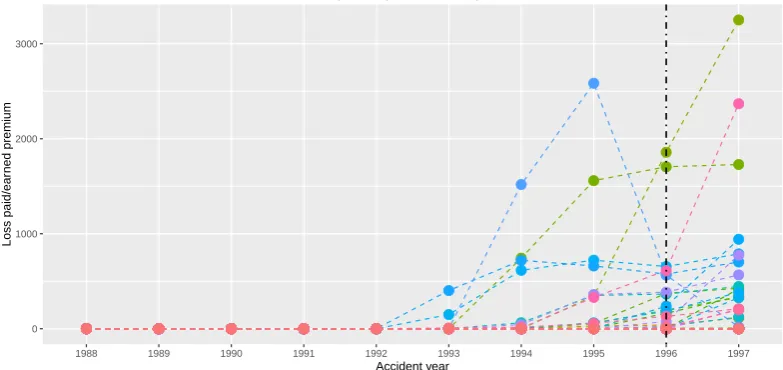
As mentioned in the introduction, our primary motivation for the change point estimation in panel data comes from the non-life insurance business. The data set is provided by the National Association of Insurance Commissioners (NAIC) database, see [16]. We concentrate on the ‘Private passenger auto liability/medical’ insurance line of business. The data collect records fromN “146 insurance companies. Each insurance company providesT “10 yearly total claim amounts starting from year 1988 up to year 1997. One can consider normalizing the claim amounts by the premium received by companyiin yeart. That is thinking of panel dataYi,t{pi,t, wherepi,tis the mentioned premium. This may yield a stabilization of series’ variability, which corresponds to AssumptionA2
of bounded variances. Figure6graphically shows series of the normalized claim amounts.
● ● ● ● ● ● ● ● ● ● ● ● ● ● ● ● ● ● ● ● ● ● ● ● ● ● ● ● ● ● ● ● ● ● ● ● ● ● ● ● ● ● ● ● ● ● ● ● ● ● ● ● ● ● ● ● ● ● ● ● ● ● ● ● ● ● ● ● ● ● ● ● ● ● ● ● ● ● ● ● ● ● ● ● ● ● ● ● ● ● ● ● ● ● ● ● ● ● ● ● ● ● ● ● ● ● ● ● ● ● ● ● ● ● ● ● ● ● ● ● ● ● ● ● ● ● ● ● ● ● ● ● ● ● ● ● ● ● ● ● ● ● ● ● ● ● ● ● ● ● ● ● ● ● ● ● ● ● ● ● ● ● ● ● ● ● ● ● ● ● ● ● ● ● ● ● ● ● ● ● ● ● ● ● ● ● ● ● ● ● ● ● ● ● ● ● ● ● ● ● ● ● ● ● ● ● ● ● ● ● ● ● ● ● ● ● ● ● ● ● ● ● ● ● ● ● ● ● ● ● ● ● ● ● ● ● ● ● ● ● ● ● ● ● ● ● ● ● ● ● ● ● ● ● ● ● ● ● ● ● ● ● ● ● ● ● ● ● ● ● ● ● ● ● ● ● ● ● ● ● ● ● ● ● ● ● ● ● ● ● ● ● ● ● ● ● ● ● ● ● ● ● ● ● ● ● ● ● ● ● ● ● ● ● ● ● ● ● ● ● ● ● ● ● ● ● ● ● ● ● ● ● ● ● ● ● ● ● ● ● ● ● ● ● ● ● ● ● ● ● ● ● ● ● ● ● ● ● ● ● ● ● ● ● ● ● ● ● ● ● ● ● ● ● ● ● ● ● ● ● ● ● ● ● ● ● ● ● ● ● ● ● ● ● ● ● ● ● ● ● ● ● ● ● ● ● ● ● ● ● ● ● ● ● ● ● ● ● ● ● ● ● ● ● ● ● ● ● ● ● ● ● ● ● ● ● ● ● ● ● ● ● ● ● ● ● ● ● ● ● ● ● ● ● ● ● ● ● ● ● ● ● ● ● ● ● ● ● ● ● ● ● ● ● ● ● ● ● ● ● ● ● ● ● ● ● ● ● ● ● ● ● ● ● ● ● ● ● ● ● ● ● ● ● ● ● ● ● ● ● ● ● ● ● ● ● ● ● ● ● ● ● ● ● ● ● ● ● ● ● ● ● ● ● ● ● ● ● ● ● ● ● ● ● ● ● ● ● ● ● ● ● ● ● ● ● ● ● ● ● ● ● ● ● ● ● ● ● ● ● ● ● ● ● ● ● ● ● ● ● ● ● ● ● ● ● ● ● ● ● ● ● ● ● ● ● ● ● ● ● ● ● ● ● ● ● ● ● ● ● ● ● ● ● ● ● ● ● ● ● ● ● ● ● ● ● ● ● ● ● ● ● ● ● ● ● ● ● ● ● ● ● ● ● ● ● ● ● ● ● ● ● ● ● ● ● ● ● ● ● ● ● ● ● ● ● ● ● ● ● ● ● ● ● ● ● ● ● ● ● ● ● ● ● ● ● ● ● ● ● ● ● ● ● ● ● ● ● ● ● ● ● ● ● ● ● ● ● ● ● ● ● ● ● ● ● ● ● ● ● ● ● ● ● ● ● ● ● ● ● ● ● ● ● ● ● ● ● ● ● ● ● ● ● ● ● ● ● ● ● ● ● ● ● ● ● ● ● ● ● ● ● ● ● ● ● ● ● ● ● ● ● ● ● ● ● ● ● ● ● ● ● ● ● ● ● ● ● ● ● ● ● ● ● ● ● ● ● ● ● ● ● ● ● ● ● ● ● ● ● ● ● ● ● ● ● ● ● ● ● ● ● ● ● ● ● ● ● ● ● ● ● ● ● ● ● ● ● ● ● ● ● ● ● ● ● ● ● ● ● ● ● ● ● ● ● ● ● ● ● ● ● ● ● ● ● ● ● ● ● ● ● ● ● ● ● ● ● ● ● ● ● ● ● ● ● ● ● ● ● ● ● ● ● ● ● ● ● ● ● ● ● ● ● ● ● ● ● ● ● ● ● ● ● ● ● ● ● ● ● ● ● ● ● ● ● ● ● ● ● ● ● ● ● ● ● ● ● ● ● ● ● ● ● ● ● ● ● ● ● ● ● ● ● ● ● ● ● ● ● ● ● ● ● ● ● ● ● ● ● ● ● ● ● ● ● ● ● ● ● ● ● ● ● ● ● ● ● ● ● ● ● ● ● ● ● ● ● ● ● ● ● ● ● ● ● ● ● ● ● ● ● ● ● ● ● ● ● ● ● ● ● ● ● ● ● ● ● ● ● ● ● ● ● ● ● ● ● ● ● ● ● ● ● ● ● ● ● ● ● ● ● ● ● ● ● ● ● ● ● ● ● ● ● ● ● ● ● ● ● ● ● ● ● ● ● ● ● ● ● ● ● ● ● ● ● ● ● ● ● ● ● ● ● ● ● ● ● ● ● ● ● ● ● ● ● ● ● ● ● ● ● ● ● ● ● ● ● ● ● ● ● ● ● ● ● ● ● ● ● ● ● ● ● ● ● ● ● ● ● ● ● ● ● ● ● ● ● ● ● ● ● ● ● ● ● ● ● ● ● ● ● ● ● ● ● ● ● ● ● ● ● ● ● ● ● ● ● ● ● ● ● ● ● ● ● ● ● ● ● ● ● ● ● ● ● ● ● ● ● ● ● ● ● ● ● ● ● ● ● ● ● ● ● ● ● ● ● ● ● ● ● ● ● ● ● ● ● ● ● ● ● ● ● ● ● ● ● ● ● ● ● ● ● ● ● ● ● ● ● ● ● ● ● ● ● ● ● ● ● ● ● ● ● ● ● ● ● ● ● ● ● ● ● ● ● ● ● ● ● ● ● ● ● ● ● ● ● ● ● ● ● ● ● ● ● ● ● ● ● ● ● ● ● ● ● ● ● ● ● ● ● ● ● ● ● ● ● ● ● ● ● ● ● ● ● ● ● ● ● ● ● ● ● ● ● ● ● ● ● ● ● ● ● ● ● ● ● ● ● ● ● ● ● ● ● ● ● ● ● ● ● ● ● ● ● ● ● ● ● ● ● ● ● ● ● ● ● ● ● ● ● ● ● ● ● ● ● ● ● ● ● ● ● ● ● ● ● ● ● ● ● ● ● ● ● ● ● ● ● ● ● ● ● ● ● ● ● ● ● ● ● ● ● ● ● ● ● ● ● ● ● ● ● ● ● ● ● ● ● ● ● ● ● ● ● ● ● ● ● ● ● ● ● ● ● ● ● ● ● 0 1000 2000 3000
1988 1989 1990 1991 1992 1993 1994 1995 1996 1997
Accident year
Loss paid/ear
ned premium
Private passenger auto liability/medical
Figure 6.Development of the yearly total claim amounts normalized by the earned premium together with the estimated change pointpτ146“9 (corresponding to year 1996).
The data are considered as panel data in the way that each insurance company corresponds to one panel, which is formed by the company’s yearly total claim amounts normalized by the earned premium. The length of the panel is quite short. This is very typical in insurance business, because considering longer panels may invoke incomparability between the early and the late claim amounts due to changing market or policies’ conditions over time.
We want to estimate a possible change in the normalized claim amounts occurred in a common year, assuming that the normalized claim amounts are approximately constant in the years before and after the possible change for every insurance company. Our change point estimator givespτ146“9 (i.e.,
year 1996) using the sequence of weightstt2u10
t“1andwp0q “ 1, which corresponds to the increased values for the last observed year 1997 shown in Figure6.
● ● ● ● ● ● ● ● ● ● ● ● ● ● ● ● ● ● ● ● ● ● ● ● ● ● ● ● ● ● ● ● ● ● ● ● ● ● ● ● ● ● ● ● ● ● ● ● ● ● ● ● ● ● ● ● ● ● ● ● ● ● ● ● ● ● ● ● ● ● ● ● ● ● ● ● ● ● ● ● ● ● ● ● ● ● ● ● ● ● ● ● ● ● ● ● ● ● ● ● ● ● ● ● ● ● ● ● ● ● ● ● ● ● ● ● ● ● ● ● ● ● ● ● ● ● ● ● ● ● ● ● ● ● ● ● ● ● ● ● ● ● ● ● ● ● ● ● ● ● ● ● ● ● ● ● ● ● ● ● ● ● ● ● ● ● ● ● ● ● ● ● ● ● ● ● ● ● ● ● ● ● ● ● ● ● ● ● ● ● ● ● ● ● ● ● ● ● ● ● ● ● ● ● ● ● ● ● ● ● ● ● ● ● ● ● ● ● ● ● ● ● ● ● ● ● ● ● ● ● ● ● ● ● ● ● ● ● ● ● ● ● ● ● ● ● ● ● ● ● ● ● ● ● ● ● ● ● ● ● ● ● ● ● ● ● ● ● ● ● ● ● ● ● ● ● ● ● ● ● ● ● ● ● ● ● ● ● ● ● ● ● ● ● ● ● ● ● ● ● ● ● ● ● ● ● ● ● ● ● ● ● ● ● ● ● ● ● ● ● ● ● ● ● ● ● ● ● ● ● ● ● ● ● ● ● ● ● ● ● ● ● ● ● ● ● ● ● ● ● ● ● ● ● ● ● ● ● ● ● ● ● ● ● ● ● ● ● ● ● ● ● ● ● ● ● ● ● ● ● ● ● ● ● ● ● ● ● ● ● ● ● ● ● ● ● ● ● ● ● ● ● ● ● ● ● ● ● ● ● ● ● ● ● ● ● ● ● ● ● ● ● ● ● ● ● ● ● ● ● ● ● ● ● ● ● ● ● ● ● ● ● ● ● ● ● ● ● ● ● ● ● ● ● ● ● ● ● ● ● ● ● ● ● ● ● ● ● ● ● ● ● ● ● ● ● ● ● ● ● ● ● ● ● ● ● ● ● ● ● ● ● ● ● ● ● ● ● ● ● ● ● ● ● ● ● ● ● ● ● ● ● ● ● ● ● ● ● ● ● ● ● ● ● ● ● ● ● ● ● ● ● ● ● ● ● ● ● ● ● ● ● ● ● ● ● ● ● ● ● ● ● ● ● ● ● ● ● ● ● ● ● ● ● ● ● ● ● ● ● ● ● ● ● ● ● ● ● ● ● ● ● ● ● ● ● ● ● ● ● ● ● ● ● ● ● ● ● ● ● ● ● ● ● ● ● ● ● ● ● ● ● ● ● ● ● ● ● ● ● ● ● ● ● ● ● ● ● ● ● ● ● ● ● ● ● ● ● ● ● ● ● ● ● ● ● ● ● ● ● ● ● ● ● ● ● ● ● ● ● ● ● ● ● ● ● ● ● ● ● ● ● ● ● ● ● ● ● ● ● ● ● ● ● ● ● ● ● ● ● ● ● ● ● ● ● ● ● ● ● ● ● ● ● ● ● ● ● ● ● ● ● ● ● ● ● ● ● ● ● ● ● ● ● ● ● ● ● ● ● 0 1000 2000 3000
1993 1994 1995 1996 1997
Accident year
Loss paid/ear
ned premium
Private passenger auto liability/medical
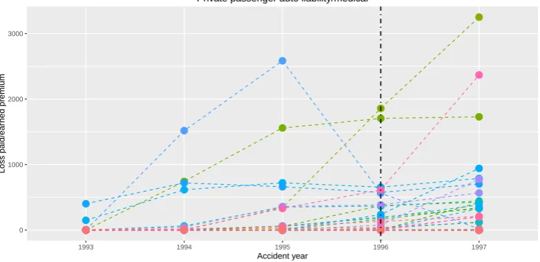
Figure 7.Development of the yearly total claim amounts normalized by the earned premium together for the second half of the original observation period with the estimated change pointτp146 “ 4 (corresponding to year 1996).
Furthermore, the empirical cumulative autocorrelation function can be obtained. The correlation matrix is estimated as proposed in Subsection5.1using the Parzen kernel
κPpxq “
$ ’ & ’ %
1´6x2`6|x|3, 0ď |x| ď1{2; 2p1´ |x|q3, 1{2ď |x| ď1;
0, otherwise.
The value of the smoothing window width is chosen ash“4. Several other values are tried from the intervalr2, 5sand all of them provide similar results. The subsequence from the empirical cumulative autocorrelation function is obtainedtprptqu10t“1“ t1.0, 2.5, 3.6, 4.6, 5.6, 6.6, 7.6, 8.6, 9.6, 10.6u.
Dependent panels may be taken into account and the presented work might be generalized for some kind of asymptotic independence over the panels or prescribed dependence among the panels. Nevertheless, our incentive is determined by a problem from non-life insurance, where the association of insurance companies consists of a relatively high number of insurance companies. Thus, the portfolio of yearly claims is so diversified, that the panels corresponding to insurance companies’ yearly claims may be viewed as independent and neither natural ordering nor clustering has to be assumed.
7. Results and Conclusions
The change point problem in panel data with fixed panel size is considered in this paper. A possible occurrence of common breaks in panel means is estimated. We introduce the change point estimator without the boundary issue meaning that it can estimate the change close to the extremities of the studied time interval. The consistency of the estimator is proved regardless of the presence/absence of the change in panel means under relatively simple conditions.
Acknowledgments: Institutional support to Barbora Peštová was provided by RVO:67985807. The research of Michal Pešta was supported by the Czech Science Foundation project GA ˇCR No. 15-04774Y.
Author Contributions: Both authors equally contributed to invention of the proposed change point estimator, to derivation its consistency, to designing and programming the simulation study, to showing its theoretical and practical applications.
Conflicts of Interest:The authors declare no conflict of interest.
Appendix Proofs
Proof of Theorem1. Let us define
SpNi,Lqptq:“ 1
wptq t
ÿ
s“1
pYi,s´Ysi,tq2, SpNi,Rqptq:“
1 wpT´tq
T
ÿ
s“t`1
pYi,s´Yri,tq2
and, consequently,SNptq:“ N1
řN
i“1
!
SpNi,Lqptq `SpNi,Rqptq
)
. Then,
SpNi,Lqptq “
$ & %
σi2 wptq
řt
s“1pεi,s´sεi,tq2, tďτ,
1 wptq
” řτ
s“1pσiεi,s´σisεi,t´
t´τ t δiq2`
řt
s“τ`1pσiεi,s´σisεi,t`
τ tδiq2
ı
, tąτ;
wheresεi,t“
1 t
řt
s“1εi,s. Similarly,
SpNi,Rqptq
“
$ ’ ’ ’ & ’ ’ ’ %
σi2 wpT´tq
řT
s“t`1pεi,s´εri,tq2, tąτ,
1 wpT´tq
” řτ
s“t`1pσiεi,s´σirεi,t´
T´τ T´tδiq2`
řT
s“τ`1pσiεi,s´σirεi,t`
τ´t T´tδiq2
ı
, tďτăT, σi2
wpT´tq
řT
s“t`1pεi,s´rεi,tq2, tďτ“T;
whererεi,t“
1 T´t
řT
s“t`1εi,sfortăTandrεi,T”0. By the definition of the cumulative autocorrelation
function, we have for 2ďtďτ
ESpNi,Lqptq “ σ
2 i wptq
t
ÿ
s“1
Epεi,s´sεi,tq
2
“ σ
2 i wptq
t
ÿ
s“1
«
1´2
t t
ÿ
r“1
Eεi,sεi,r` 1 t2rptq
ff
“ σ
2 i wptq
ˆ
t´rptq
t
˙
.
Clearly,SpNi,Lqp1q “0. In the remaining case whentąτ, one can calculate
ESpNi,Lqptq “ σ
2 i wptq
ˆ
t´rptq
t
˙
` τ
wptq
ˆ
t´τ t
˙2
δi2`t´τ
wptq
´τ
t
¯2
δ2i
“ σ
2 it wptq
ˆ
1´rptq
t2
˙
`τpt´τq
twptq δ
2 i.
By the definition of an empty sum,SpNi,RqpTq “0 and, moreover,SNpi,RqpT´1q “0. ForT´1ątąτ,
ESpNi,Rqptq “ σ
2 i wpT´tq
T
ÿ
s“t`1
Epεi,s´rεi,tq
2
“ σ
2 i wpT´tq
T
ÿ
s“t`1
«
1´ 2
T´t T
ÿ
r“t`1
Eεi,sεi,r` 1
pT´tq2rpT´tq
ff
“ σ
2 i wpT´tq
ˆ
T´t´rpT´tq
T´t
˙
The same result is obtained forT“τąt. In the remaining caseT´1ěτětsuch thatT´1ąt,
ESpNi,Rqptq “ σ
2 i wpT´tq
ˆ
T´t´rpT´tq
T´t
˙
` τ´t
wpT´tq
ˆ
T´τ T´t
˙2
δ2i ` T´τ
wpT´tq
ˆ
τ´t T´t
˙2
δi2
“σ
2 ipT´tq wpT´tq
ˆ
1´rpT´tq pT´tq2
˙
` pτ´tqpT´τq pT´tqwpT´tqδ
2 i.
Realize thatSpNi,Lqptq `SpNi,Rqptq ´ESpNi,Lqptq ´ESpNi,Rqptqare independent with zero mean for fixed tandi“1, . . . ,N, but they are not identically distributed. Due to AssumptionA5and the stochastic Cauchy-Schwarz inequality, fortďτăTit holds
VarSNptq “ 1 N2
N
ÿ
i“1
#
σi4 w2ptqVar
« t ÿ
s“1
pεi,s´sεi,tq
2
ff
` 1
w2pT´tqVar
«
σi2 τ
ÿ
s“t`1
pεi,s´rεi,tq
2
´2T´τ T´tσiδi
τ
ÿ
s“t`1
pεi,s´rεi,tq ` ˆ
T´τ T´t
˙2
δi2
`σi2 T
ÿ
s“τ`1
pεi,s´rεi,tq
2
`2τ´t T´tσiδi
T
ÿ
s“τ`1
pεi,s´rεi,tq ` ˆ
τ´t T´t
˙2
δ2i
ff
` 2σ
2 i
wptqwpT´tqCov
« t ÿ
s“1
pεi,s´sεi,tq
2, σi2
τ
ÿ
s“t`1
pεi,s´rεi,tq
2´2T´τ T´tσiδi
τ
ÿ
s“t`1
pεi,s´rεi,tq
`
ˆ
T´τ T´t
˙2
δ2i `σi2 T
ÿ
s“τ`1
pεi,s´rεi,tq
2
`2τ´t T´tσiδi
T
ÿ
s“τ`1
pεi,s´rεi,tq ` ˆ
τ´t T´t
˙2
δi2
ff+
ď 1
NC1pt,τ,σ,σq ` 1
N2C2pt,τ,σ,σq N
ÿ
i“1 δ2i ` 1
N2C3pt,τ,σ,σq
ˇ ˇ ˇ ˇ ˇ N ÿ i“1 δi ˇ ˇ ˇ ˇ ˇ ,
whereC1pt,τ,σ,σq ą 0, C2pt,τ,σ,σq ě 0, andC3pt,τ,σ,σq ě 0 are some constants not depending onN. Iftăτ“T, then
VarSNptq “ 1 N2
N
ÿ
i“1
#
σi4 w2ptqVar
« t ÿ
s“1
pεi,s´sεi,tq
2
ff
` σ
4 i w2pT´tqVar
« T ÿ
s“t`1
pεi,s´rεi,tq
2
ff
` 2σ
4 i
wptqwpT´tqCov
« t ÿ
s“1
pεi,s´sεi,tq
2, T
ÿ
s“t`1
pεi,s´rεi,tq
2
ff+
ď 1
NC4pt,τ,σ,σq, whereC4pt,τ,σ,σq ą 0 does not depend on N. In case of t “ τ “ T, we also haveVarSNpTq ď
1
NC5pT,τ,σ,σq, whereC5pT,τ,σ,σq ą0 does not depend onN. Finally iftąτ, then
VarSNptq “ 1 N2
N
ÿ
i“1
#
σi4 w2pT´tqVar
« T ÿ
s“t`1
pεi,s´rεi,tq
2
ff
` 1
w2ptqVar
«
σi2 τ
ÿ
s“1
pεi,s´sεi,tq
2
´2t´τ t σiδi
τ
ÿ
s“1
pεi,s´sεi,tq ` ˆ
t´τ t
˙2
δ2i `σi2 t
ÿ
s“τ`1
pεi,s´sεi,tq
2
`2τ tσiδi
t
ÿ
s“τ`1
pεi,s´sεi,tq ` ´τ
t
¯2
δ2i
ff
` 2σ
2 i
wpT´tqwptqCov
« T ÿ
s“t`1
pεi,s´rεi,tq
2, σi2
τ
ÿ
s“1
pεi,s´sεi,tq
2
´2t´τ t σiδi
τ
ÿ
s“1
`
ˆ
t´τ t
˙2
δi2`σi2 t
ÿ
s“τ`1
pεi,s´sεi,tq
2
`2τ tσiδi
t
ÿ
s“τ`1
pεi,s´sεi,tq ` ´τ
t
¯2
δi2
ff+
ď 1
ND1pt,τ,σ,σq ` 1
N2D2pt,τ,σ,σq N
ÿ
i“1 δ2i ` 1
N2D3pt,τ,σ,σq
ˇ ˇ ˇ ˇ ˇ N ÿ i“1 δi ˇ ˇ ˇ ˇ ˇ ,
whereD1pt,τ,σ,σq ą0,D2pt,τ,σ,σq ě0, andD3pt,τ,σ,σq ě0 do not depend onN. The Chebyshev inequality providesSNptq ´ESNptq “ OP
´a
VarSNptq
¯
asN Ñ 8. According to AssumptionA4
and the Cauchy-Schwarz inequality, we have
1 N2 ˇ ˇ ˇ ˇ ˇ N ÿ i“1 δi ˇ ˇ ˇ ˇ ˇ ď 1 N g f f e1 N N ÿ i“1
δi2Ñ0, NÑ 8.
Since the index sett1, . . . ,Tuis finite andτis finite as well, then
max
1ďtďTVarSNptq ď 1
NK1pσ,σq `K2pσ,σq 1 N2
N
ÿ
i“1
δ2i `K3pσ,σq 1
N2 ˇ ˇ ˇ ˇ ˇ N ÿ i“1 δi ˇ ˇ ˇ ˇ ˇ ď 1
NK4pσ,σq,
whereK1pσ,σq ą0,K2pσ,σq ě0,K3pσ,σq ě0, andK4pσ,σq ą0 are constants not depending onN. Thus, we also have uniform stochastic boundedness, i.e.,
max
1ďtďT|SNptq ´ESNptq| “OP
ˆ
1 ?
N
˙
, NÑ 8.
Adding and subtracting, one has
SNptq ´SNpτq “SNptq ´ESNptq ´ rSNpτq ´ESNpτqs `ESNptq ´ESNpτq ě ´2 max
1ďrďT|SNprq ´ESNprq| `ESNptq ´ESNpτq “ ´2 max
1ďrďT|SNprq ´ESNprq| ` 1 N
˜N ÿ
i“1 σi2
¸ «
t wptq
ˆ
1´rptq
t2
˙
´ τ
wpτq
ˆ
1´rpτq
τ2
˙
`IttăTu T´t
wpT´tq
ˆ
1´rpT´tq pT´tq2
˙
´ItτăTu T´τ
wpT´τq
ˆ
1´rpT´τq pT´τq2
˙ff ` 1 N ˜N ÿ i“1 δi2
¸„
Ittąτuτpt´τq
twptq `Ittăτu
pτ´tqpT´τq pT´tqwpT´tq
(5)
for eachtP t1, . . . ,Tu. Particularly, inequality (5) holds forpτN. Note thatτpN “arg mintSNptq. Hence,
SNppτNq ´SNpτq ď0. Therefore,
2?N max
1ďrďT|SNprq ´ESNprq| (6)
ě
„
ItτpNąτu
τpτpN´τq p
τNwpτpNq
`ItτpNăτu
pτ´pτNqpT´τq
pT´τpNqwpT´τpNq 1 ? N N ÿ i“1 δi2
`
« p
τN wpτpNq
˜
1´rpτpNq
p
τN2
¸
´ τ
wpτq
ˆ
1´rpτq
τ2
˙
`ItpτNăTu
T´pτN
wpT´τpNq ˆ
1´rpT´τpNq pT´pτNq2
˙
´ItτăTu T´τ
wpT´τq
ˆ
1´rpT´τq pT´τq2
˙ff 1 ? N N ÿ i“1 σi2
“ItτpNąτu
1 ?
N
#
τpτpN´τq p
τNwpτpNq
N
ÿ
i“1
δ2i ` rgppτNq ´gpτq `gpT´pτNq ´gpT´τqs
N
ÿ
i“1 σi2
`ItpτNăτu
1 ?
N
#
pτ´τpNqpT´τq
pT´pτNqwpT´τpNq
N
ÿ
i“1
δi2` rgppτNq ´gpτq `gpT´pτNq ´gpT´τqs
N
ÿ
i“1 σi2
+
ěItτpNąτu
1 ?
N
#
τ wppτNq
ˆ
1´ τ
p
τN
˙ N ÿ
i“1
δi2´ rgpτq `gpT´τqs N
ÿ
i“1 σi2
+
`ItpτNăτu
1 ?
N
#
T´τ wpT´pτNq
ˆ
1´ T´τ
T´pτN ˙ N
ÿ
i“1
δ2i ´ rgpτq `gpT´τqs N
ÿ
i“1 σi2
+
ěItτpNąτu
1 ?
N
#
τ
pτ`1qmaxt“1,...,Twptq N
ÿ
i“1
δ2i ´ rgpτq `gpT´τqs N
ÿ
i“1 σi2
+
(7)
`ItpτNăτu
1 ?
N
#
T´τ
pT´τ`1qmaxt“1,...,Twptq N
ÿ
i“1
δ2i ´ rgpτq `gpT´τqs N
ÿ
i“1 σi2
+
, (8)
wheregptq “ wt
ptq
´
1´rpt2tq
¯
ě0 fort P t1, . . . ,Tuand gp0q ”0. Since expression in (6) isOPp1qas NÑ 8, we haveItτpN ą τu
P
Ñ 0 as well asItpτN ăτu
P
Ñ0 due to AssumptionsA3applied in (7) and (8). Hence,PrτpN “τs Ñ1 asNÑ 8.
Proof of Theorem2. (i)Let us define
UNptq:“ N ÿ i“1 t ÿ s“1
pYi,s´µiq.
Using the multivariate Lyapunov CLT for a sequence ofT-dimensional independent random vectors
"
σi
” ř1
s“1εi,s, . . . ,řTs“1εi,s
ıJ*
iPN
, we have underH0
Σ´1{2
N rUNp1q, . . . ,UNpTqsJÝÝÝÝÑD
NÑ8 rX1, . . . ,XTs J, such that ΣN“ N ÿ i“1 σi2Var
« 1 ÿ
s“1 εi,s, . . . ,
T
ÿ
s“1 εi,s
ffJ
“ς2NΛ,
where Λ “ Var
” ř1
s“1ε1,s, . . . ,
řT s“1ε1,s
ıJ
is positive definite covariance matrix with respect to
AssumptionA1and 0ă Nσ2 ď ς2N :“řNi“1σi2 ď Nσ2 according to AssumptionA2. The limiting T-dimensional random vector rX1, . . . ,XTsJ has multivariate normal distribution with zero mean and identity covariance matrix. The Lyapunov condition is satisfied due to the Jensen inequality, the Cramér-Wold theorem, and AssumptionA5, i.e.,
´
aJΣNa¯´ 2`χ
2 ÿN
i“1 E ˇ ˇ ˇ ˇ ˇ ˇ
aJσi
« 1 ÿ
s“1 εi,s, . . . ,
T
ÿ
s“1 εi,s
ffJˇˇ ˇ ˇ ˇ ˇ
2`χ
“ς´2´N χ
´
aJΛa¯´ 2`χ
2 ÿN
i“1 σi2`χE
ˇ ˇ ˇ ˇ ˇ T ÿ t“1 at t ÿ s“1 εi,s
ˇ ˇ ˇ ˇ ˇ 2`χ
ďT1`χς´2´χ N
´
aJΛa
¯´2`χ 2 ÿN
i“1 σi2`χ
T ÿ t“1 E ˜ at t ÿ s“1 εi,s
¸2`χ
ďT1`χς´2´N χ
´
aJΛa
¯´2`χ 2 ÿN
i“1 σi2`χ
T
ÿ
t“1
|at|2`χt1`χ t
ÿ
s“1
ď$ς´2´N χ N
ÿ
i“1
σi2`χď$
´
Nσ2¯´ 2`χ
2
Nσ2`χ“
$σ´2´χσ2`χN´ χ
2 Ñ0, NÑ 8 (9)
for arbitrary fixed0‰a“ ra1, . . . ,aTsJPRTand some 0ăχď2, where
$“T1`χ´aJΛa¯´ 2`χ
2 ÿT
t“1
|at|2`χt1`χ t
ÿ
s“1
E|ε1,s|2`χ
is a positive constant not depending onN. Thet-th diagonal element of the covariance matrixΛis
Var
t
ÿ
s“1
ε1,s“rptq
and the upper off-diagonal element on positionpt,vqis
Cov
˜ t ÿ
s“1 ε1,s,
v
ÿ
u“1 ε1,u
¸
“Var
t
ÿ
s“1
ε1,s`Cov
˜ t ÿ
s“1 ε1,s,
v
ÿ
u“t`1 ε1,u
¸
“rptq `Rpt,vq, tăv.
Moreover, let us define the reverse analogue ofUNptq, i.e.,
VNptq:“ N
ÿ
i“1 T
ÿ
s“t`1
pYi,s´µiq “UNpTq ´UNptq.
Hence,
UNpsq ´s
tUNptq “ N
ÿ
i“1
# s ÿ
r“1
« `
Yi,r´µi
˘
´1
t t
ÿ
v“1
`
Yi,v´µi
˘ ff+
“ N
ÿ
i“1 s
ÿ
r“1
`
Yi,r´Ysi,t ˘
and, consequently,
VNpsq ´ T´s
T´tVNptq “ N
ÿ
i“1
# T ÿ
r“s`1
« `
Yi,r´µi
˘
´ 1
T´t T
ÿ
v“t`1
`
Yi,v´µi
˘ ff+
“ N
ÿ
i“1 T
ÿ
r“s`1
´
Yi,r´Yri,t ¯
,
fortăT. Then, underH0
r
Σ´1{2N rVNp1q, . . . ,VNpT´1qsJÝÝÝÝÑD
NÑ8 rZ1, . . . ,ZT´1s J,
whereZt:“XT´Xtand
r
ΣN“ N
ÿ
i“1 σi2Var
« T ÿ
s“2 εi,s, . . . ,
T
ÿ
s“T εi,s
ffJ
“ς2NΛr
forΛr “Var ”
řT
s“2ε1,s, . . . ,
řT s“Tε1,s
ıJ
. Using the continuous mapping theorem, we end up with
SN,TÝÝÝÝÑD NÑ8 L such that the lawLcorresponds to the distribution of
S
˜ !
Xs´s tXt
)t´1,T
s“1,t“1,
"
Zs´T ´s T´tZt
*T´1,T´1 s“t,t“1
¸
(ii)Let us definepei,t:“ řt
s“1pei,s,pe
˚ i,t:“
řt s“1pe
˚ i,s,
p
UNptq:“ N ÿ i“1 t ÿ s“1 p
ei,s“ N
ÿ
i“1
p
ei,t,
and
p
U˚Nptq:“ N ÿ i“1 t ÿ s“1 p
Yi˚,s “ N ÿ i“1 t ÿ s“1 ˜ pe ˚ i,s´
1 N N ÿ i“1 p
ei,s
¸ “ N ÿ i“1 t ÿ s“1 ` p
e˚i,s´pei,s ˘ “ N ÿ i“1 ` p
e˚i,t´pei,t ˘
.
Realize thatpei,tdepends onτpNand, hence, it depends onN.
Let us calculate limNÑ8Γi,N, whereΓi,N“Varrpei,1, . . . ,pei,Ts
J. Using the law of total variance,
Varpei,t“ErVartpei,t|pτNus `VarrEtepi,t|pτNus “
T
ÿ
π“1
PrpτN“πsVarrepi,t|τpN “πs
` T
ÿ
π“1
PrτpN“πstErpei,t|τpN“πsu
2
´
# T ÿ
π“1
PrpτN“πsErepi,t|pτN“πs +2
.
Since limNÑ8PrτpN“τs “1 andErpei,t|pτN“τs “0, then
lim NÑ8
Varpei,t“ lim
NÑ8
Varrpei,t|τpN“τs.
Similarly with the covariance, i.e., after applying the law of total covariance, we have
lim NÑ8Cov
` p
ei,t,pei,v ˘
“ lim NÑ8Cov
`
pei,t,pei,v|τpN“τ ˘
.
Note that
` p
ei,t|pτN“τ ˘
“
#
σipεi,t´εsi,τq, tďτ; σipεi,t´εri,τq, tąτ; where sεi,t “
1 t
řt
s“1εi,s and rεi,t “
1 T´t
řT
s“t`1εi,s. Taking into account the definitions of rptq and Rpt,vq together with some simple algebra, we obtain that Varrpei,s|τpN “ τs “ σi2γt,tpτq and
Cov`pei,t,pei,v|pτN“τ ˘
“σi2γt,vpτqfortăvsuch that
γt,tpτq “
$ ’ ’ & ’ ’ %
rptq ` t2 τ2rpτq ´
2t
τrrptq `Rpt,τqs, tăτ; 0, t“τ;
rpt´τq ` pt´τq2
pT´τq2rpT´τq ´ 2pt´τq
T´τ rrpt´τq `Rpt´τ,T´τqs, tąτ; and
γt,vpτq “
$ ’ ’ ’ ’ ’ ’ & ’ ’ ’ ’ ’ ’ %
0, t“τorv“τ, rptq `Rpt,vq ` tv
τ2rpτq ´ v
τrrptq `Rpt,τqs ´ t
τrrpvq `Rpv,τqs, tăvăτ; Spt,v,τ`1´tq ` tpv´τq
τpT´τqRpτ,Tq ´ v´τ
T´τSpt,T,τ`1´tq ´ t
τRpτ,vq, tăτăv; rpt´τq `Rpt´τ,v´τq `pt´τqpv´τq
pT´τq2 rpT´τq ´ v´τ
T´τrrpt´τq `Rpt´τ,T´τqs ´t´τ
T´τrrpv´τq `Rpv´τ,T´τqs, τătăv; where
Spt,v,dq “Cov
˜ t ÿ
s“1 εi,s,
v
ÿ
u“t`d εi,u
¸ “ t ÿ s“1 v ÿ
u“t`d
Thus, limNÑ8Γi,N “ σi2Γpτq, where the matrix Γpτq “ tγt,vpτquTt,v,T“1 is symmetric and does not depend oni. The matrixΓpτqis singular. Nevertheless, omitting theτ-th row and theτ-th column fromΓpτq, one obtains matrix rΓpτq, i.e., rΓpτq :“ Γ´τ,´τpτq, which has a full rank ofT´1 due to AssumptionA1and
` p
ei,t|τpN“τ ˘
“
$ ’ ’ & ’ ’ %
σi
´ řt
s“1εi,s´tsεi,τ
¯
, tăτ;
0, t“τ;
σi
´ řt
s“τ`1εi,s´ pt´τqrεi,τ
¯
, tąτ. Let us define random vectors
UN:“ rUNp1q, . . . ,UNpτpN´1q,UNppτN`1q, . . . ,UNpTqs
J,
p
UN:“ rUpNp1q, . . . ,UpNpτpN´1q,UpNppτN`1q, . . . ,UpNpTqsJ, p
U˚
N:“ rUp˚Np1q, . . . ,UpN˚pτpN´1q,Up˚NppτN`1q, . . . ,Up˚NpTqsJ,
i.e., they do not contain elements with argumentτpN. The law of total probability provides
P
„
ς´1N rΓ
´1{2
pτqUp˚Nďx ˇ ˇY
´P
„
ς´1N rΓ
´1{2
pτqUNp ďx
“ T
ÿ
π“1
"
P
„
ς´1N rΓ
´1{2
pτqUp˚Nďx ˇ
ˇY,pτN“π
´P
„
ς´1N rΓ
´1{2
pτqUNp ďx ˇ ˇ pτN“π
*
PrpτN“πs (10)
for all x P RT. Since Assumption A5 holds, then according to the bootstrap multivariate CLT by [17, Theorem 2.4] for (conditionally) independent and not identically distributed zero mean T-dimensional random vectorsξN “
“
rpei,1, . . . ,pei,TsJ ˇ
ˇ pτN “τ‰, we have
P
„
ς´1N rΓ
´1{2
pτqUp˚Nďx ˇ
ˇY,τpN“τ
´P
„
ς´1N rΓ
´1{2
pτqUNp ďx ˇ ˇ pτN“τ
P
ÝÝÝÝÑ
NÑ8 0 (11)
for allxPRT. Theorem1, relations (10) and (11) imply
P
„
ς´1N rΓ
´1{2
pτqUp˚Nďx ˇ ˇY
´P
„
ς´1N rΓ
´1{2
pτqUpNďx
P
ÝÝÝÝÑ
NÑ8 0 (12)
for allxPRT.
Using the law of total probability again, we obtain
P
„
ς´1N rΓ
´1{2
pτqUpNďx
“ T
ÿ
π“1
P
„
ς´1N rΓ
´1{2
pτqUpNďx ˇ ˇ pτN“π
PrτpN“πs. (13)
The consistency result limNÑ8PrτpN“τs “1 from Theorem1and equation (13) give
P
„
ς´1N rΓ
´1{2
pτqUNp ďx
´P
„
ς´1N rΓ
´1{2
pτqUNp ďx ˇ ˇ pτN“τ
P
ÝÝÝÝÑ
NÑ8 0. (14)
Since the Lyapunov CLT provides that
„
ς´1N rΓ
´1{2
pτqUNp ďx ˇ ˇ pτN“τ
has an approximate