http://www.sciencepublishinggroup.com/j/sjams doi: 10.11648/j.sjams.20190705.11
ISSN: 2376-9491 (Print); ISSN: 2376-9513 (Online)
Multi-Step Game of Reserves Management in the
Attack-Defense Model
Alexander Gennadievich Perevozchikov
1, Valery Yurievich Reshetov
2, Igor Evgenievich Yanochkin
11Center for Complex System Modeling, RusBitekh-Tver', Tver', Russia 2
Faculty of Computational Mathematics and Cybernetics, Lomonosov Moscow State University, Moscow, Russia
Email address:
To cite this article:
Alexander Gennadievich Perevozchikov, Valery Yurievich Reshetov, Igor Evgenievich Yanochkin. Multi-Step Game of Reserves Management in the Attack-Defense Model. Science Journal of Applied Mathematics and Statistics. Vol. 7, No. 5, 2019, pp. 63-70. doi: 10.11648/j.sjams.20190705.11
Received: July 24, 2019; Accepted: September 22, 2019; Published: October 11, 2019
Abstract:
The authors describe a multi-step generalization of the “attack-defense” model, defined and studied by Germeier. It is a modification of the Gross’ model. The similar model was proposed by Gorelik for the gasoline production. In the military models the points are usually interpreted as directions and characterize the spatial distribution of defense resources across the width of the defense front. The dynamics of the average number of parties described by the “attack-defense” game can be described by finite-difference Osipov-Lanchester’ equations. Therefore, it would also be interesting to obtain a generalization of Germeyer’s classical model to the dynamic case when the “attack-defense” game is played many times. On this basis, in the present work, a dynamic expansion of the model is constructed in the form of a positional game with opposing interests of the distribution of parties’ reserves with complete information. The authors studied the simplest multi-step extension of the attack-defense model, which consists in the fact that the corresponding game is played repeatedly. Multi-step game with the complete information of the parties’ reserves management was built on this basis. It is assumed that the defense party makes the first move at each step and the attack party became aware about this move. The functional equation for the best guaranteed result of the defense, which is the value of the positional game due to the parties’ adopted sequence of moves was written out. Its analytical solution for a two-step game was obtained and it was shown that it is advantageous for an attack party to enter all reserves simultaneously, as in the classic attack-defense game.Keywords:
Attack-Defense Game, Multi-Step Expansion of the Game, Guaranteed Defense Result, Game Value, Optimal Attack Strategy, Optimal Defense Strategy1. Introduction
The authors describe a multi-step generalization of the attack-defense game, defined and studied by Germeier [1]. It is a modification of the Gross’ model [2] and it is the basis for the authors’ further constructions. A similar model was proposed by Gorelik for the gasoline production [3]. The game model, generalizing the Gross’ and Germeier’ models was studied in the work [4]. In military models points are usually interpreted as directions and characterize the spatial distribution of defense resources across the width of the defense front. It is also possible to distribute the resources in depth associated with the separation of the defense. The parties’ resources are heterogeneous in general case. All these areas of generalization of the classical “attack-defense”
model have been studied by the authors in previous works [5-8], which can be considered as the authors’ modest contribution to the available literature on these issues. In reality, there is also a multistep continuation of the conflict in the form of a sequence of strikes inflicted before a sufficient level of losses is achieved by one of the parties (exhaustion) that is incompatible with the continuation of the conflict. The dynamics of the average number of parties in a multi-step conflict described by the “attack-defense” game was studied in the work [9]. System’s dynamics was described by finite-difference Osipov-Lanchester’ equations.
discrete optimal control problem and can be solved by the gradient descent method with averaging. The control problem posed in the work [6] clarifies the problem of the distribution of defense resources in a given direction by levels in terms of accounting for more general restrictions than in the work [5], which take into account the possibility of the use of defense means at various borders. In the work [7], a generalization of the “attack-defense” model was studied, which consists in taking into account the heterogeneity of the parties’ means using target distribution based on the classical transport problem. Article [8] summarizes the classical game “attack-defense” in terms of accounting for the defense topology that has a network structure and is based on the work by Hohzaki and Tanaka [10]. In contrast to the latter, the defense at each of the possible directions of movement between the vertices of the network defined by oriented edges can have several boundaries, which made it possible to combine the classes of multilevel and network models.
In practical terms, it would also be interesting to obtain a generalization of the Germeyer’s classical model [1] to the dynamic case when the “attack-defense” game is played many times. In the work [9], a special case was considered when the use of parties’ reserves during the repetition of the game was not supposed. On this basis, in the present work, a dynamic expansion of the model is constructed in the form of a positional game with opposite interests of the distribution of the parties' reserves with complete information. The functional equation for the best guaranteed result of defense, which is the value of the positional game due to the adopted sequence of moves of the parties, in which the defense party make the first move at each, was written out. The analytical solution of this equation is given for the case of a two-step game, it has the practical importance, since the attack party usually plans no more than two attacks per day on defense party. Written in normal form, this game refers to hierarchical games Γ1 (see [1]) in the particular case when the interests of the players are opposite. The classic “attack-defense” game is the simplest discrete analogue of the average dynamics model, so the authors did not use statistical methods in the work, remaining within the framework of deterministic models.
Adaptive control in repetitive hierarchical games Γ1 with non-opposite interests was studied in [11]. Repeated hierarchical games Γ2 with non-opposite interests were studied in [12, 13]. Dynamic quasi-information expansions of games with an expandable coalition structure were discussed in [14]. One class of repetitive games with incomplete information is described in [15].
2. The Basic Game of Attack-Defense
The basic for our formulations attack-defense game was studied in the work [1]. This game can be formulated as follows. Let Pi−the probability of hitting of one means of
attack with one means of defense in the i− direction,
1,...,
i
=
n
. It is required to solve an antagonistic game with the function of attack’s winning, which represents the average number of penetrated means of attack:{
}
1
( , ) max 0,
n
i i i i
f X U X PU
=
=
∑
− (1)Let V and Y - the number attack’s and defense’s means. The defense strategy is to distribute its funds in the directions of defense in accordance with the vector:
{
}
1
1
( ,..., ) , 0, 1,...,
n
n i i
i
U U U A U U V U i n
=
= ∈ =
∑
= ≥ = (2)The attack strategy is to distribute its funds in the directions in accordance with the vector:
{
}
1
1
( ,..., ) , 0, 1,...,
n
n i i
t
X X X B X X Y X i n
=
= ∈ =
∑
= ≥ = (3)Using the convexity of the function f X U( , )onU , for this antagonistic game it was proved in particular (see, for example, [16], pp. 61-64) that the minimax:
(
( ))
1,...,
( , ) ,
minmax
min
max
iU A
U A X B i n
f X U f X U
v
∈
∈ ∈ =
=
=
(4)will be the value of the game and the minimax defense strategy is optimal. Here X( )i =(0,...,X,...0), where X is in the i-th place, and the rest of the coordinates are zero. In this case, the optimal attack strategy is a mixed strategy, consisting in concentrating all forces in one direction in accordance with the optimal probability distribution, which can be obtained using the formulas also given in the work [16]. These formulas will be required for further exposition, therefore we will give them in full.
The minimax strategy, which is the optimal pure defense strategy, has the form
1
* , 1, 2,..., 1
i n i
i i
V
U i n
P P
=
= =
∑
(5)The corresponding best guaranteed defense result is
1
1
1 max(0; ( ) )
n
i i
v Y V
P
−
=
= −
∑
(6)and is the value of the game.
( )
0 0 0
0
1 1
, 1, 0, 1, 2,...,
i
n n
i X i i
i i
p I p p i n
φ
= =
=
∑
∑
= ≥ = ,where IX( )i - is a probability measure concentrated at a point
( )i
X . Then the optimal strategy is the strategy φ0, when pi0
is determined by the formula
0 1
1
1 1
( ) , 1, 2,...,
n i
i i i
p i n
P P
−
=
=
∑
= . (7)3. The Simplest Multi-step Model of
“Attack-Defense”
Let us denote by Y Vt, tthe average amount of the sides’ means at the end of t-th strike, which is modeled by playing the basic attack-defense game, then the equation for the average value∆Yt in the absence of reserves follows from
equation (6).
1
1 0
1 1
min( ; ( ) ), 0,1,..., .
n t t t t t
i i
Y Y Y Y V t Y Y
P
− +
=
∆ = − = −
∑
= = (8)To obtain the equation for the average value∆Vt, let’s consider the i-th direction,
i
=
1,...,
n
. Let Ri−the probability ofhitting of one means of defense with one means of attack on the i−th direction,
i
=
1,...,
n
. By analogy with (8) it can be assumed, following [9], that the average losses will be in accordance with formula (5)1
1 1
min( ; ( ) ).
n
i t
t i t
i i i
V
V R Y
P P
−
=
∆ = −
∑
(9)Now the total average losses can be found as the mathematical expectation (9) taking into account the probability distribution (7)
1 1
1
1 1 1
1 1 1
( ) min( ; ( ) ).
n n n
t
t t t i t
i i i i
i i i
V
V V V R Y
P P P P
− −
+
= = =
∆ = − = −
∑ ∑
∑
(10)Let’s write equations (8), (10) as
1
1 0
1 1
max(0; ( ) ), 0,1,... 1, .
n
t t t
i i
Y Y V t T Y Y
P
− +
=
= −
∑
= − = (11)and
1 1
1 0
1 1 1
1 1 1 1
( ) max( [1 ( ) ]; ); ;
n n n
t t t i t
i i i i
i i i
V V V R Y V V
P P P P
− −
+
= = =
=
∑ ∑
−∑
− = (12)where t - is the number of attack’ strike, which determines the time step of the discrete model, T - is the specified planning horizon.
Let’s suppose that at the beginning of each strike, the sides exchange blows of long-range weapons. We denote m the probability of maintaining the combat capability of one unit of attack or defense. Let ut(vt ) - is the number of reserve means of attack (defense) entered from safe shelters in the t
-th step. The total number of reserves of attack and defense, we denote respectively by Q and W .
Let’s subdue the reserves to conditions
1
0
, 0, 0,1,..., 1,
T
t t t
u Q u t T
−
=
≤ ≥ = −
∑
(13)and
1
0
, 0, 0,1,..., 1.
T
t t t
v W v t T
−
=
≤ ≥ = −
∑
(14)Then the equations of system motion can be written as
1
1 0
1 1
max(0; ( )( ) ), 0,1,... 1, .
n t t t t t
i i
Y mY u mV v t T Y Y
P
− +
=
1 1
1 0
1 1 1
1 1 1 1
( ) max{( ) [1 ( ) ]; ( )}, 0,1,... 1,;
n n n
t t t t t i t t
i i i i
i i i
V mV v mV v R mY u t T V V
P P P P
− −
+
= = =
=
∑ ∑
+ ×× −∑
+ − + = − = (16)Let’s write equations 15, 16) in general form
1 ( , , , ), 0,1,..., 1, 0 ,
t t t t t
Y+ = f Y V u v t= T− Y =Y (17)
and
1 ( , , , ), 0,1,..., 1, 0 ,
t t t t t
V+ =g Y V u v t= T− V =V (18)
We introduce the additional phase variables Y Vt0, t0, subduing them to the equations
0 0 0
1 , 1,..., 1, 0 0,
t t t
Y+ =Y +u t= T− Y = (19)
and
0 0 0
1 , 1,..., 1, 0 0,
t t t
V+ =V +v t= T− V = (20)
Then the constraints (13), (9) on the control actions ut(vt ) can be written as
{
}
0 1 0
( ) 0 , 0,1,..., 1,
t t t t t
u ∈R Y = u ∈E ≤u ≤ −Q Y t= T− (21)
and
{
}
0 1 0
( ) 0 , 0,1,..., 1.
t t t t t
v ∈P V = v ∈E ≤v ≤ −W V t= T− (22)
The multivalued mappings Yt0 →R Y( t0)and Vt0 →P V( t0)
will be Hausdorff’s continuous by virtue of Lemma 1.4 in [17, p.30] in the areas 0≤Yt0 ≤Q and 0≤Vt0 ≤W , respectively.
Let’s take the average number of attack means that overcame defense taking into consideration the repeated strikes as an attack win
1
([ ],[ ]) T t t t
t
J u v Y
=
=
∑
. (23)The defense win will be the reciprocal
([ t],[ ])t ([ t],[ ])t
I u v = −J u v
4. The Positional Game of the Reserves’
Distribution
Let’s consider the positional game of the reserves’ distribution using the constructed dynamic expansion of the target distribution model.
The game starts from the position(Y V Y V0, 0, 00, 00). At the initial moment of discrete time, the players of the attack and the defense make a choice of control actions
0 0
0 ( 0), 0 ( 0 )
u ∈R Y v ∈P V . In this case, the defense party make the fist move and the attack party became aware about this
choice. In normal form, this corresponds to the game logic G1
(see [1]) in the particular case when the interests of the players are opposite. In the position (Y V Y Vt , t , t0, t0) the players choose ut ∈R Y( t0),vt ∈P V( t0)and the attack party became aware about the defense’s choice vt ∈P V( t0) before the choice ut ∈R Y( t0). The process ends in the (T−1)-th step by the choice uT−1∈R Y( T0−1),vT−1∈P V( T0−1) and transition to the state(Y V Y VT, T, T0, T0).
Let’s [Yt ]=( ,...,Y1 YT) - the trajectory of attack, implemented in the game. The winning of the attack party is determined by the formula (23), the winning of the defense party is opposite in sign to the winning of the attack party.
We will assume that the game is a game with complete information, i.e. at each step, the players know the position
0 0
(Y V Y Vt , t , t , t ) and the point of the discrete time
0,...,
1
t
=
T
−
, and the attack party additionally knows the choice of the defense partyvt ∈P V( t0).Attack strategies are all sorts of functions 0 0
( , , , , , )
u Y V Y V v t , such thatu Y V Y V v t( , ,t t t0, t0, , )t ∈R Y( t0). Defense strategies are all sorts of functions v Y V Y V t( , , 0, 0, ), such that v Y V Y V t( , ,t t t0, t0, )∈P V( t0) . These strategies are called pure.
0 0
( , , , , , )
u Y V Y V v t and v Y V Y V t( , , 0, 0, ) . In the situation ( (.), (.))u v the game is as follows. At the t -th step,
0,...,
1
t
=
T
−
, the system moves from the state0 0
(Y V Y Vt, t, t , t ) to the state defined by equalities
0 0 0 0 0 0
1 ( , , ( , , , , ( , , , , ), ), ( , , , , )), 0,1,..., 1, 0
t t t t t t t t t t t t t t t
Y+ = f Y V u Y V Y V v Y V Y V t t v Y V Y V t t= T− Y =Y
and
0 0 0 0 0 0
1 ( , , ( , , , , ( , , , , ), ), ( , , , , ), 0,1,..., 1, 0
t t t t t t t t t t t t t t t
V+ =g Y V u Y V Y V v Y V Y V t t v Y V Y V t t= T− V =V
for the main phase variables and
0 0 0 0 0 0 0
1 ( , , , , ( , , , , ), ), 0,1,..., 1, 0 0,
t t t t t t t t t t
Y+ =Y +u Y V Y V v Y V Y V t t t= T− Y =
and
0 0 0 0 0
1 ( , , , , ), 0,1,..., 1, 0 0,
t t t t t t
V+ =V +v Y V Y V t t= T− V =
for additional phase variables.
Thus, each situation ( (.), (.))u v uniquely corresponds to the trajectory [Yt ]=( ,...,Y1 YT) of the attack and therefore the win, determined by the formula (23)
1
(( (.), (.)) ([ ],[ ])
T
t t t
t
L u v J u v Y
=
= =
∑
, (24)The considered game depends on two parameters - on the starting position (Y V Y V0, 0, 00, 00) and duration T. Therefore, we denote it by G(Y0, V0, Y00, V00, T). To obtain a functional equation for the value V Y V Y V T( 0, 0, 00, 00, )of a game G(Y0, V0, Y00, V00, T), it is convenient to immerse it in a family of
games G(Yt, Vt, Yt0, Vt0, T – t) of value
0 0
( t , t , t , t , )
V Y V Y V T−t
By virtue of the continuity of functions f Y V u v( , , , ), ( , , , )
f Y V u v with respect to the totality of variables and Hausdorf’s continuity of multivalued mappings Yt0→R Y( t0)
and Vt0→P V( t0)like Theorem 7 in the work [18, p. 38], it is established by induction
t
= −
T
1,..., 0
that the following result come around.Theorem 1. Games G(Yt, Vt, Yt0, Vt0, T – t) has equilibrium
situations in pure strategies. Moreover, its values
0 0
( t , t , t , t , )
V Y V Y V T−t satisfy the functional equation
0 0
0 0
( ) ( )
0 0
0 0
( , , , , ) min max [ ( , , , ) ( ( ( , , , ),
( , , , ), , , 1)]; 1,..., 0; ( , , , , 0) 0.
t t t t
t t t t t t t t t t t t v P V u R Y
t t t t t t t t T T T T
V Y V Y V T t f Y V u v V f f Y V u v
g Y V u v Y u V v T t
t T V Y V Y V
∈ ∈
− = + +
+ + − −
= − =
(25)
This theorem generalizes the Zermelo’s theorem for finite games with complete information. To solve the functional equation (25), grid-based methods are applied (see [18]), the convergence of which to the solution requires separate study and is not discussed here.
The written functional equation for the value of the positional game gives the best guaranteed defense result, which is the value of the game due to the adopted sequence of moves, in which the defense party make the first move at each step. This game written in normal form is related to hierarchical games G1 (see [1]) in the particular case when
the interests of the parties are opposite.
5. Analytical Solution of a Two-Step
Game
Let's suppose that T=2. First we’ll consider a particular case n=1, and then we’ll return to the general case.
Then the equations of system motion are the usual discrete equations of the Osipov-Lanchester’s model [9] of the dynamics of the average and can be written as
1 max(0; ( ) ), 0,1; 0 .
t t t t t
Y+ = mY + −u mV +v P t= Y =Y (26)
and
1 max(0; ( )), 0,1; 0 ,
t t t t t
V+ = mV + −v R mY +u t= V =V (27)
where indicated for brevity sake
1, 1
P=P R=R .
0 0
1 1 1 1
0 0 0 0 0 0
1 1 1 1 1 1 1 1 1 1 1 1 1 1 1 1
0 0
( , , , ,1) min max ( , , , ) ( , , , ) max(0; ( ) ).
v W V u Q Y
V Y V Y V f Y V u v f Y V Q Y W V mY Q Y mV W V P
≤ ≤ − ≤ ≤ −
= = − − = + − − + −
The latter is true because the nondecreasing function 1 1 1 1
( , , , )
f Y V u v on u1 and nonincreasing on v1 (см.(26)). Now from the equation (25) we get
0 0
0 0 0 0 0 0
0 0
0 0
0 0 0 0 0 0 0 0 0 0 0 0
( , , 0, 0, 2) min max [ ( , , , )
( ( , , , ), ( , , , ), , ,1)]
v W u Q
V Y V f Y V u v
V f Y V u v g Y V u v Y u V v
≤ ≤ ≤ ≤
= +
+ + +
or expanded
0 1
0 0
0 0
0 0 0
0 0 0
( , , 0, 0, 2) min max {max[0; ( ) ] max(0; max[0; ( ) ]
( max[0; ( ] )}.
v W u Q
V Y V mY u mV v P
m mY u mV v P Q u
P m mV v R mY u W v
≤ ≤ ≤ ≤
= + − + + + + − + + − −
− + − + + −
(28)
We obtain the condition under which
1 max(0; 0 ( 0) ) 0
Y = mY+u − mV+v P > .
This condition is equivalent to the inequality
0 0( 0) 0 ( )
u >u v =Pv −m Y−PV . (29)
If (29) is satisfied, then under the sign of the minimax in (28) stands the function
1 0 0 0 0
0 0 0 0
0 0
( , ) max{ ( ) ;
(1 )[ ( ) ]
max[0; ( ]}.
F u v mY u mV v P
m mY u mV v P Q u PW Pv
Pm mV v R mY u
= + − +
+ + − + + − − + −
− + − +
(30)
If (30) is not satisfied, then under the sign of the minimax in (29) stands the function
0 0 0 0 0
0 0
( , ) max{0;
max[0; ( ]}.
F u v Q u PW Pv
Pm mV v R mY u
= − − + −
− + − + (31)
Thus, under the minimax sign in (29) stands the function
1 0 0 0 0 0
0 0
0 0 0 0 0 0
( , ), ( ) ( , )
( , ), ( )
F u v u u v
F u v
F u v u u v
>
=
≤
It is not difficult to verify that the following lemma holds. Lemma 2. The function F u v1( 0, 0) (F u v0( 0, 0) increases on u0 and does not increase on v0 (decreases on u0and increases on v0).
Corollary 1. From Lemma 2 it follows that for any v0 value u0 can take only two values 0 and Q. This means that it is beneficial for an attack party to enter all reserves simultaneously, either in the first step or in the second.
Let’s introduce the notations
* (Y ); ** Q (Y )
W m V W m V
P P P
= − = + − . (32)
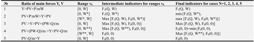
Different ways of calculating the game’s value arise in connection with the position of the point u v0( )0 as relating to the segment [0, ]Q . In addition, it is important the difference sign Q−PW, showing whether the defense party is able to destroy the entire reserve of attack party by its reserve. Analysis of options and indicators from which you need to find the maximum are shown in Tables 1 and 2.
Table 1. Options and indicators, the minimax of which gives the game value at Q−PW<0.
N Ratio of main forces Y, V Range v0 Intermediate indicators for ranges v0 Final indicators for cases N=1, 2, 3, 4, 5
1 Y>PV+P/mW [0, W] F1(Q, W) F1(Q, W)
2 PV+P/mW>Y>PV+(PW-Q)/m [0, W*] F1(Q, W*) Min {F1(Q, W*),
max [F1(Q, W), F0(0, W*)]}
[W*, W] Max [F1(Q, W), F0(0, W*)]
3 PV+(PW-Q)/m>Y>PV
[0, W*] F1(Q, W*) Min {F1(Q, W*),
Max [F1(Q, W**), F0(0, W*)],
F0(0, W**)}
[W*, W**] Max [F1(Q, W**), F0(0, W*)]
[W**, W] F0(0, W**)
4 PV>Y>PV-Q/m [0, W**] Max [F1(Q, W**), F0(0, 0)] Min {max [F1(Q, W**), F0(0, 0)], F0(0, 0)}=F0(0, 0)
[W**, W] F0(0, 0)
5 PV-Q/m>Y [0, W] F0(0, 0) F0(0, 0)
The boundaries of the ranges can be attributed to the right or to the left range, the result of calculating the game value will be the same. The final indicators are obtained by minimizing the intermediate indicators for the ranges.
Table 2. Options and indicators, the minimax of which gives the value of the game at.
№ Ratio of main forces Y, V Range v0 Intermediate indicators for ranges v0 Final indicators for cases N=1, 2, 3, 4, 5
1 Y>PV+P/mW [0, W] F1(Q, W) F1(Q, W)
2 PV+P/mW>Y>PV [0, W*] F1(Q, W*) min{F1(Q, W*),
max [F1(Q, W), F0(0, W*)]}
[W*, W] Max [F1(Q, W), F0(0, W*)]
3 PV >Y>PV+(PW-Q)/m [0, W] Max [F1(Q, W), F0(0, 0)] Max [F1(Q, W), F0(0, 0)]
4 PV+(PW-Q)/m >Y>PV-Q/m [0, W**] Max [F1(Q, W**), F0(0, 0)] F0(0, 0)=min{F0(0, 0), Max [F1(Q, W**), F0(0, 0)]}
[W**, W] F0(0, 0)
Remark 2. The values of the arguments of the indicator on which the minimax is implemented give optimal values v u0, 0. In the general case, the equations of dynamics has the form (15), (16)
1 max(0; ( ) , 0,1,... 1, 0 .
t t t t t
Y+ = mY + −u mV +v P t= T− Y =Y (33)
and
1 1
0
max(( ) ; ( )),
0,1,... 1,; .
n
t i t t i t t i t t i
V p mV v q mV v R mY u
t T V V
+ =
= + + − +
= − =
∑
(34)
where indicated for short
1
1
1 1
( ) ), , 1
n
i i i
i i
i
P p P q p
P P
−
=
=
∑
= = −In this case, the expression (28) for the game price will have the form
0 1
0 0
0 0
0 0 0
0 1
( , , 0, 0, 2) min max {max[0; ( ) ]
max(0; max[0; ( ) ]
( max(( ) ; ( )) )}.
v W u Q
n
i t t i t t i t t i
V Y V mY u mV v P
m mY u mV v P Q u
P m p mV v q mV v R mY u W v
≤ ≤ ≤ ≤
=
= + − + +
+ + − + + − −
−
∑
+ + − + + −(35)
The functions F F1, 0 defined by formulas (30, 31) will undergo similar changes.
1 0 0 0 0
0 0 0 0
1
( , ) max{ ( ) ;
(1 )[ ( ) ]
max(( ) ; ( ))}
n
i t t i t t i t t i
F u v mY u mV v P
m mY u mV v P Q u PW Pv
Pm p mV v q mV v R mY u
=
= + − +
+ + − + + − − + −
−
∑
+ + − +(36)
and
0 0 0 0 0
1
( , ) max{0;
max(( ) ; ( ))}.
n
i t t i t t i t t i
F u v Q u PW Pv
Pm p mV v q mV v R mY u
=
= − − + −
−
∑
+ + − + (37)After this, Lemma 2 and Corollary 1 remain valid. The game value and the optimal values u v0, 0 are obtained from Tables 1 and 2, depending on the ratio of reserves.
6. Conclusion
The authors describe in this paper a multi-step generalization of the “attack-defense” model, defined and studied by Germeier. In the military models the points are usually interpreted as directions and characterize the spatial distribution of defense resources across the width of the defense front. It is also possible to distribute the resources in depth in relation with the separation of the defense. The parties’ resources are heterogeneous in general case. All these areas of generalization of the classical “attack-defense” model have been studied by the authors in previous works. In reality, there is also a multistep continuation of the conflict in the form of a sequence of strikes inflicted before
a sufficient level of losses is achieved by one of the parties (exhaustion) that is incompatible with the continuation of the conflict. Therefore, in this paper, the authors constructed the model's dynamic extension in the form of a positional game with opposing interests of the parties' reserves distribution with complete information. The analytical solution of this extersion was obtained for two-step game; that has practical value as the attack party plans usually no more than two strikes in a day on the defense party. And it was shown that it is advantageous for an attack party to enter all reserves simultaneously, as in the classic attack-defense game.
References
[2] Karlin S. Mathematical methods in game theory, programming and economics. Moscow, Mir, 1964.
[3] Gorelik V. A. Game Theory and Operations Research. Moscow, Publishing House MINGP, 1978.
[4] Ogaryshev V. F. Mixed strategies in a single generalization of the Gross’ problem// Journal of computational mathematics and mathematical physics, 1973. V. 13. No. 1. pp. 59-70. [5] Reshetov V. Y., PtrevozchikovA. G., Lesik I. A. A Model of
Overpowering a Multilevel Defense System by Attak// Computational Mathematics and Modeling, 2016, Vol. 27, No. 2, p. 254-269.
[6] Reshetov V. Y., PtrevozchikovA. G., Lesik I. A. Multi-Level Defense System Models: Overcoming by Means of Attacks with Several Phase Constraints//Moscow University Computational Mathematics and Cybernetics, 2017, Vol. 1, No. 1, p. 25-31.
[7] Reshetov V. Y., PtrevozchikovA. G., Yanochkin I. E. An Attack-Defense Model with Inhomogeneous Resources of the Opponents//Computational Mathematics and Mathematical Physics, 2018, Vol. 58, No. 1, p. 38-47.
[8] Reshetov V. Y., PtrevozchikovA. G., Yanochkin I. E. Multilayered Attack-Defense Model on Networks//Computational Mathematics and Mathematical Physics, 2019, Vol. 59, No. 8, p. 1389-1397.
[9] Reshetov V. Y., Perevozchikov A. G, Lesik A. I. Multistep generalization of the attack-defense model//Bulletin of Tver State Univercity. Seria Applied Mathematics. 2017, No. 2. pp. 12-24. [10] Hohzaki R., Tanaka V. The effects of players recognition about
the acquisition of his information by his opponent in an attrition game on a network//In Abstract of 27th European
conference on Operation Research 12-15 July 2015 University of Strathclyde. - EURO2015.
[11] Molodtsov D. A. Adaptive control in repetitive games// Journal of computational mathematics and mathematical physics, 1978. Vol. 18, No. 1, pp. 78-83.
[12] Danilchenko T. N., Masevich K. K. Multistage game of two persons with a “cautious” second player and consistent transmission of information// Journal of Computational Mathematics and Mathematical Physics, 1974. V. 19. No. 5. pp. 1323-1327.
[13] Ereshko F. I., Propoi A. I. To the theory of dynamic games. News of the USSR Academy of Sciences. Techical cybernetics. 1970, No. 2, pp. 42-47.
[14] Krutov B. P. Dynamic quasi-informational extensions of games with an expandable coalition structure. Moscow, CC of RAS, 1986.
[15] Vatel I. A., Dranev Y. N. About one class of repetitive games with incomplete information in a two-level economic system. In Proceedings of International conference "Modeling of economic processes." Moscow, CC of the USSR Academy of Sciences, 1975, pp. 224-238.
[16] Vasin A. A., Morozov V. V. Game theory and models of mathematical economics. Moscow, MAX Press, 2005. [17] Fedorov V. V. Maximin’s numerical methods. Moscow,
Science, 1979.