An evolutionary classifier for steel surface defects with small sample set

R E S E A R C H

Open Access

An evolutionary classifier for steel surface

defects with small sample set

Mang Xiao

, Mingming Jiang

, Guangyao Li

, Li Xie

and Li Yi

Abstract

Nowadays, surface defect detection systems for steel strip have replaced traditional artificial inspection systems, and automatic defect detection systems offer good performance when the sample set is large and the model is stable. However, the trained model does work well when a new production line is initiated with different equipment, processes, or detection devices. These variables make just tiny changes to the real-world model but have a significant impact on the classification result. To overcome these problems, we propose an evolutionary classifier with a Bayes kernel (BYEC) that can be adjusted with a small sample set to better adapt the model for a new production line. First, abundant features were introduced to cover detailed information about the defects. Second, we constructed a series of support vector machines (SVMs) with a random subspace of the features. Then, a Bayes classifier was trained as an evolutionary kernel fused with the results from the sub-SVM to form an integrated classifier. Finally, we proposed a method to adjust the Bayes evolutionary kernel with a small sample set. We compared the performance of this method to various algorithms; experimental results demonstrate that the proposed method can be adjusted with a small sample set to fit the changed model. Experimental evaluations were conducted to demonstrate the robustness, low requirement for samples, and adaptiveness of the proposed method.

Keywords: Surface defect, Support vector machine, Random subspace, Bayes classifier

1 Introduction

With the growth in competition among producers of steel strip, the quality of the steel strip surface has become very important. Steel strip quality and the surface quality of structural products have assumed increasingly signif-icant importance [1]. The importance of surface quality requires that effective and efficient methods be imple-mented to replace conventional artificial visual inspection during which an expert can only inspect 0.05% of the total steel surface, which can be easily impacted by fatigue and other unfavorable conditions. Artificial inspection cannot satisfy the quality requirements. Therefore, auto-matic, high-accuracy steel surface inspection systems have become essential to the production system.

Surface defect inspection systems mainly consist of two parts: defect segmentation and defect processing. Defect processing entails feature extraction and defect classification. In recent years, abundant research has been

*Correspondence: [email protected]

2_{Department of Electronics and Information Engineering, Tongji University,} Shanghai, China

Full list of author information is available at the end of the article

conducted, and different kinds of feature extraction and classification methods have been introduced to classify steel strip surface defect. In [2, 3], the defects were classified by using K-nearest neighbor (KNN) methods with a co-occurrence matrix. Santanu Ghorai et al. [4] described an automated visual inspection system with dis-crete wavelet transform (DWT) features and a support vector machine (SVM). Wu et al. [5] described an algo-rithm with an undecimated wavelet transform (UWT) and a mathematical morphology to detect geometric defects that achieved a 90.23% accuracy that is difficult to achieve in real industrial application in 2008. However, in 2013, a noise-robust method based on a completed local binary proposed by Song [6] averaged 98% accuracy and was shown to be effective enough to be applied to real produc-tion. A review of vision-based steel surface inspection sys-tems [1] indicates that most such syssys-tems have achieved >90% accuracy.

For application to real production, some difficulties for steel surface defect detection remain. In a real production environment, different products can be produced on a sin-gle production line, and some products are manufactured

on several production lines at the same time. With the passage of time, the physical conditions of the equip-ment and of the detection device will both change. Each of these variables has only a small impact on the real-world model; however, the classifier trained by the original database will not work well on the changed real-world model. If we trained every production line and every prod-uct with a single database, it would take a long time for a steel company to get a large enough sample set for a newly built production line without a trained inspection system.

Unfortunately, most research has focused on algorithms that work only when a large number of samples is avail-able, there little research has focused on this production problem. Solly et al. proposed a rapidly evolving sys-tem with an expert’s feedback; however, that research describes an adaptive interactive evolution methodology for determining parameters to control segmentation of surface defects on images, and the classification accu-racy will still be impacted by changing the real-world model.

Therefore, to solve these issues, we propose an evo-lutionary classifier with a Bayes kernel (BYEC) that can be adjusted with small sample sets to fit the changed model. Because the small changes to the real-world model will impact some features of the clas-sifier, the misclassification of the classifier is mainly impacted by these features. Nevertheless, if we reduce the impact of these features, we should be able to restore the classifier to get a relatively high accuracy [7]. Thus, we built a classic classifier with an evolutionary Bayes kernel and adjusted the kernel with a small sam-ple set for the changed production model rather than training every product and every production line with a single data set.

Our technical contribution includes three points. First, we propose an evolutionary classifier with a Bayes kernel (BYEC) for steel defect classification. Second, we adopt multiple SVMs to predict individual features, enabling our evolutionary Bayes kernel to fit well with a small sample set for the changed production model. Third, and most importantly, we combine five selected fea-tures and prove that our method has high accuracy, is adaptive, and has a low requirement for samples in our experiments.

The rest of the paper is organized as follows: Section 2 depicts the procedures of the surface defect inspection system. Section 3 presents the features we used in this paper. The method to build SVM subclassifiers on a ran-dom subspace of features is provided in Section 4. The method to build the Bayes kernel and evolve the ker-nel is discussed in Section 5. Section 6 gives compara-tive experimental results of this algorithm and research on factors that affect the results. Finally, we conclude

this paper in Section 7 and give some suggestions for future work.

2 Structure of the evolutionary classifier for steel surface defects

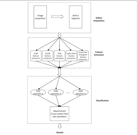
An evolutionary surface defect inspection system should be trained as a classic classifier and evolve to fit the changed real world on the real production line with a small sample set. The structure of the inspection sys-tem is presented in Fig. 1. Our syssys-tem mechanism mainly involves three processes: defect acquisition, fea-ture extraction, and defect classification.

The image acquisition system has been discussed in much of the literature [8–10] and has become a mature field, so we will not discuss it in this paper again.

As it illustrated in the Fig. 1, five kinds of features were introduced in this system. The reason of this is because the penalize of some features in the adjust-ment process drop some useful information of the defect and may lead to misclassification, so superfluous features were imported. We integrated the uniform local binary patterns (ULBP) [11], gray-level co-occurrence matrix (GLCM) features [12], the histogram of oriented gradient (HOG) feature, and gray-level histogram and Gabor fil-ter features. These abundant features guarantee enough information for the classifier. To utilize these features, a multiple classifier system was imported into this classifier. The classification part has two components in Fig. 1: multiple SVM classifiers and a Bayes kernel classifier. Compared with the classic steel surface inspection system, the fuser Bayes kernel makes the key contribution to this system by fusing the results from the multiple classifiers and adjusting the hybrid parameters.

The SVM [13] is a popular small sample set learning method. It offers very good performance for pat-tern classification problems by minimizing the Vapnik-Chervonenkis (VC) dimension and achieving a minimal structural risk. Because of its small sample set require-ment, fast learning capability, and good performance, SVM is a good choice for this method. Because each SVM classifier is trained by a subspace of the feature space, we can evaluate and penalize the features by using the corresponding SVM classifier.

Fig. 1Structure of the evolutionary classifier for steel surface defects using a Bayes kernel

in time so that future data may be badly processed if we maintain the same classification. Drift decreases the accu-racy of the classification result, the individual classifier evaluation is done on their accuracy on the new data. The best performing classifiers are selected to constitute the MCS committee after every loop. Kolter et al. [15] described a dynamic weighted majority algorithm. We also use an evolvable weighted method to change our classifier with time.

The method to fuse the subclassifiers must be adjusted with a small sample set and the accuracy of the subclas-sifiers must be evaluated; therefore, the Bayes classifier

is a good candidate as it builds a reference from prior probability to posterior probability. We can score the per-formance of the classifiers on the changed model by the posterior probability. With a small sample set, we can get the approximate posterior of the classifiers and use it to reweight the integrated classifier to fit the real model. A Bayes kernel was built based on this concept.

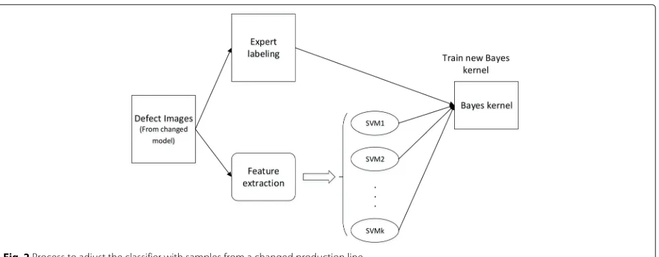
Fig. 2Process to adjust the classifier with samples from a changed production line

used to train the Bayes kernel classifier. This Bayes clas-sifier is combined with the multiple SVM clasclas-sifiers as an integrated classifier.

3 Extraction of features

To avoid the lack of information after integration, we introduce redundant features to overcome this weakness. Five different kinds of features are extracted in the inspec-tion system to describe the properties of texture, color, and shape, respectively. The feature space consists of a gray-level co-occurrence matrix, a uniform local binary pattern, a histogram of oriented gradient, a gray-level histogram, and a Gabor filter.

3.1 Gray-level co-occurrence matrix

Gray-level co-occurrence matrix is aNg×Ngmatrix where

Ng is the number of gray levels in the image, this matrix

reflects the direction, adjacent distance, and change range of the image. Every value in the matrix represents a joint probability that two gray-level pixels exist with a distance ofdand a directionθ, it is defined in Eq. 1. Where matrix C is computed over an n × m image I , d and θ are described by x andythat x = sin(θ)× d, y = cos(θ)×d. Whereiandjare the image intensity values of the image,pandqare the spatial positions in the image.

Cx,y(i,j)= p=1

n q=1

m

1, ifI(p,q)=iandI(p+x,q+y)=j

0, otherwise

(1)

The GLCM is sensitive to rotation, so we choose four directions 0°, 45°, 90°, and 135° to cover more information and select a distance of 8. The dimensions of the GLCM is too large for us to process, so we choose Haralick features [12] to describe it which calculates the correlation, energy,

contrast, entropy, and inertia quadrature of the GLCM. Finally, we get a vector to describe the GLCM feature.

3.2 Histogram of oriented gradient and gray level The histogram is a key tool in image processing, it is one of the most useful techniques in gathering information about a matrix. The gray-level histogram of the defect image represents the distribution of the pixels over the gray-level scale and reflects the contrast, gray level, and other infor-mation of the image. It can be visualized as if each pixel is placed in a bin corresponding to the color intensity of that pixels. We make the histogram of the defect image to 40 bins and turn it into a feature vector as the gray-level feature.

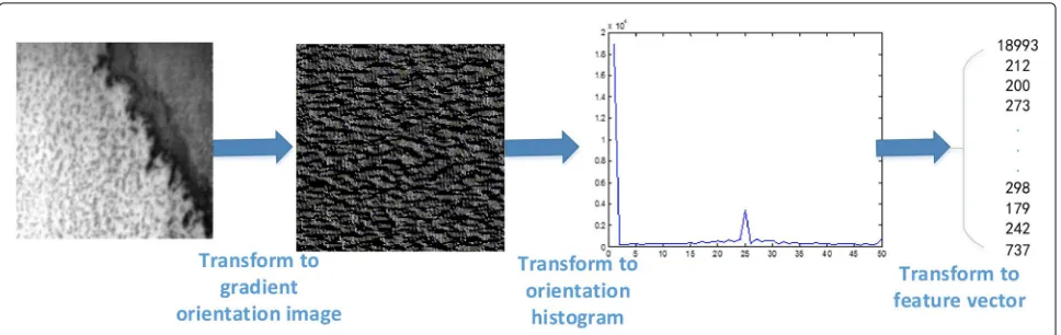
Dalal Navneet and Triggs Bill proposed the histogram of oriented gradient in 2005 [16], this feature is used in com-puter vision and image processing for object detection, which counts the occurrences of the oriented gradient in an image. The image can be described by the distribution of intensity gradients and edge directions. In convention-ally procedure, the image is divided into many small cells and calculated respectively, but in this paper, we make the histogram on the whole picture.

Gx=H(x+1,y)−H(x−1,y)

Gy=H(x,y+1)−H(x,y−1)

G(x,y)=

Gx(x,y)2+Gy(x,y)2

α(x,y)=tan−1

Gy(x,y)

Gx(x,y)

(2)

Equation 2 defines the gradient orientation and value, Gx is the gradient value ofxorientation,Gyis the

Fig. 3Process to convert defect image to HOG feature vector

then we make the histogram of the image with 50 chan-nels. Finally, we get the value of every bin and convert it to a feature vector to represent the HOG.

3.3 Uniform local binary pattern

The local binary pattern (LBP) is one of the most success-ful statistical approaches for texture classification due to its gray-scale and rotation invariance, this feature reflects the local texture of the image. LBP filter is a 3×3 win-dow. As it defined in Eq. 3, the gray level of the center pixel is set as the threshold, gray value of the adjacent 8 pixels around center pixel is compared with the threshold. If the value of a surrounding pixel is larger than the threshold, the position of this pixel is marked as 1, otherwise 0.

LBPP= P−1

p=0

s(gp−gc)2p,s(x)=

1 ifx0

0 ifx<0 (3)

One local binary filter can produce 2pdifferent values, and this dimension is too high for us to process. Ojala [11] proposed ULBP to reduce the dimension of the LBP. ULBP introduces a uniformity measureUwhich corresponds to the number of spatial transitions (between [0, 1]) in the pattern. For example, U(000000012) and U(000000102)

equal 2 as they have two transitions between [0, 1] . The Uvalue of most LBPs is not greater than 2, and the num-ber of these LBPs is 57. The ULBP is defined as Eq. 4, a unique id is assigned to a pattern that itsU value is not greater than 2, so we reduce the dimension from 256 to 58. As Fig. 4 described, to get the ULBP feature, firstly, we convert the defect image to a ULBP image and then we make the histogram of the ULBP image and convert the histogram to a feature vector.

ULBPP=

id(LBP) ifU(LBP(x))2

58 ifU(LBP(x)) <2 (4)

3.4 Gabor filter

The Gabor filter is used for edge detection in image pro-cessing, the frequency and orientation representations of

Gabor filters are similar to those of the human visual system and efficient to describe the texture. Its impulse response is defined by a sinusoidal wave multiplied by a Gaussian function. Because of the multiplication convolution property (Convolution theorem), the Fourier transform of a Gabor filter’s impulse response is the con-volution of the Fourier transform of the harmonic func-tion and the Fourier transform of the Gaussian funcfunc-tion. The filter has a real and imaginary component represent-ing orthogonal directions [17]. We only take the real part of the Gabor filter in this paper. The real Gabor filter kernel is defined as Eq. 5.

g(x,y;λ,θ,ψ,σ,γ )=exp

−x ₂

+λ2_y2

2θ2

cos

2πx

λ +ψ

(5)

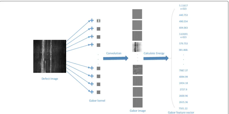
λ is the wavelength of the sinusoidal factor, θ repre-sents the orientation of the normal to the parallel stripes of the Gabor function,ψrepresents the phase offset of the sinusoidal function,σ represents the sigma deviation of the Gaussian envelope, andγ represents the spatial ratio. As depicted in Fig. 5, in this paper, we make a Gabor fil-ter bank withλ(2, 3, 4, 5, 6)andθ 0,1₈π,2₈π,3₈π,4₈π,5₈π,

6 8π,78π

, totally with 40 Gabor filter kernels, and apply convolution on the defect image with these Gabor filters and get 40 Gabor images. We make a Gabor feature vector composed of the energy of these Gabor images.

4 The SVM subclassifiers on a random subspace of features

Fig. 4Process to convert defect image to ULBP feature vector

subspace. We choose a feature subspace with the ran-dom sampling scheme rather than with a feature category or in sequence for two reasons: (1) the feature punished will involve features nearby that may contain some useful information and not interfered by the real-world model, and (2) features nearby may contain the same information and the classifier will not get a good result with nearby features.

To overcome the small sample set issue on the produc-tion line, we introduce a support vector machine, which

has been widely used in many areas, such as computer vision, natural language processing, and neuroimaging, for its good performance, fast training capability, and small sample set requirements for labeled samples.

There are six kinds of defects in the database which we used for the experiment, as SVM is a binary classifier, we implemented the multiclass classification with the “one-against-one” scheme which is usually applied for binary classifier [18, 19]. For every multiclass SVM classifier in this paper, the number of binary SVM classifiers we need

is defined as Eq. 6, thekis the number of classes exists in data set.

nSVM=k(k−1)/2 , wherek≥1. (6)

Corinna describes the standard SVM for two classifica-tions in [20] within the structural risk minimization. The key of SVM is to find the hyperplane to minimize the distance between the two classes to be separated.

With a training vectorsxi ⊆ Rn,i = 1,. . .,l, belong to

two classes, and vectory⊆Rlsuch thatyi ⊆ {1,−1}

indi-cate the class of the corresponding data, the SVM try to solve the following minimization problem in Eq. 7:

min

w,b,ξ

1 2w

T_w+C l

i=1

ξi

subject toyi

wTφ(xi)+b

≥1−ξi

ξi≥0,i=1,. . .,l,

(7)

theξiis a map function which mapsxiinto higher feature

space make the points easily to be separated andC>0 is the regularization parameter,wis the weight vector for the feature space. To solve the possible high dimensionality of the vectorw, we usually convert it to the dual problem as Eq. 8 presents:

min

α

1 2α

T_Qα−eT_α

subject toyTα=0,

0≤αi≤C, i=1,. . .,l.

(8)

In which e = [1,. . ., 1]T is the vector of all ones, Q represents anl by l positive semidefinite matrix, Qij ≡

yiyjK(xi,xj), and K(xi,xj) ≡ φ(xi)Tφ(xj) is the kernel

function.

Then, the problem is solved with the primal dual rela-tionship, we can calculate thewwith Eq. 9.

w=

l

i=1

yiαiφ(xi) (9)

Finally, we can classify the data points with the Eq. 10:

sgnwTφ(x)+b=sgn ⎛

⎝l

i=1

yiαiK(xi,x)+b ⎞

⎠. (10)

For the classification ofith andjth classes, we solve it with the Eq. 11 deduced from Eq. 7.

min

wij_,bij_,ξij

1 2w

ijT_wij_+C

t

ξij t

subject towijTφ(xt)+bij≥1−ξtij, ifxtin theith class

wijTφ(xt)+bij≥1−ξtij, ifxtin thejth class

ξij

t ≥0 (11)

We combine the results from the binary classifier with a voting scheme: every binary classifier has a vote, and a data point is classified into the class with the maximum number of votes. To solve the clash of the same votes, we simply choose the class with the greater sequence num-ber. In addition, we increase the sequence number for the classes with every multiclass SVM to avoid accumulated deviations. A simple example indicates the risks without this strategy: Assume we have three classes,A,B, andC, all with the same accuracy and scale. Then, samples classified intoAare least.

5 Combining subclassifiers by using the Bayes kernel

The combination of the subclassifiers is very important to this evolutionary classifier because it not only response for improving the performance of the final integrated clas-sifier but also for the ability to evolve itself to fit the new changed model. Many ensemble methods have been presented [21–23]; however, these methods do not suit this adaptive inspection system. This is because (1) these methods are sensitive to the size of the training sample set (although, even for a mature production line, there are not too many labeled samples), and (2) the fusion of classifiers may be biased from the combination of samples from the changed model.

For these reasons, we propose a new fusion strategy based on a native Bayes classifier. This is a highly practi-cal Bayesian learning method deduced from the Bayesian theorem

P(Bi|A)= _nP(Bi)P(A|Bi)

i=1P(Bi)P(A|Bi) (12)

This theorem was proposed for about 300 years by Thomas Bayes 12 and has developed into a great branch of machine learning. In some domains, it is presented as comparable to neural networks and to other machine learning methods. The naive Bayes classifier f(x) is described by a conjunction of attribute values when the f(x) is limited to a finite setV.

In Bayes learning, the training examples are described by a feature vector (a1,a2,a3. . .an)T; the Bayes

classi-fier makes decisions based on the probability for every possible value and selects the most portable target.

In this model, we assign every subclassifier as a fea-ture in the feafea-ture vector and described it as a prob-ability matrix. The feature vector of the Bayes vector is defined as (D1,D2,D3. . .Dm)T, the Di is the

The prior probability that theith classifier make decision kand the real class isjis defined as Eq. 13.

P(R=j|Di=k)=

1 m

m

i=1

1 ifDi=kandR=j

0 otherwise

(13)

The variable m describes the number of the samples; then, we can deduce the post probability of the decisionj, that theith classifier make decisionk, defined by Eq. 14:

P(Di=k|R=j)=

P(R=j|Di=k)

n

l=1P(R=j|Di=l)

. (14)

The advisable number of decisions that the classifier can make is defined by the variable n. With this post prob-ability for every individual classifier, the Bayes classifier can make decisions based on a multinomial model [24]. The naive Bayes classifier uses the simplifying assump-tions that the attribute values are conditionally indepen-dent and that individual classifiers are indepenindepen-dent in this model. The probability of observing the conjunction of classifiersD1,D2,D3. . .Dmis just the product of the post

probability of the individual classifiers, in which case, our Bayes classifier will make a decision based on Eq. 15.

v=argmax

vl∈V

P(R=l)

m

i=0

P(R=l|Di) (15)

The key structure of the naive Bayes fusion kernel in this model is the post probability matrix for individual classi-fiers that we trained with labeled samples. To adjust our model to fit the changed real-world model, we changed the post probability matrix.

As depicted in Fig. 2, to evolve the Bayes kernel, a new post probability matrix was trained to replace the old one with the labeled samples from the changed production line. The new classifier model is combined by the naive Bayes kernel with a new post probability matrix and SVM subclassifiers. The Bayes classifier takes advantage of not only the true positive result but also the true negative result from the subclassifiers. Because some subclassi-fiers may lose efficacy after a real-world model change and make a biased classification, this message can also be utilized by the integrated classifier.

6 Experimental results

To evaluate the effectiveness of the inspection system for surface defects, a surface defect data set was used. We then compared this approach with some other classification methods. In addition, some factors were examined that demonstrate how they affected classifica-tion accuracy.

6.1 Experiment implementation details

The accuracy of this evolutionary classifier has been compared with other classifiers such as SVM [25], NN-BP [26], and KNN [3]. To reveal the fairness of the clas-sifier, a surface defect database, the NEU surface defect database1 [6] was used. There are six kinds of typical defects of the hot-rolled steel strip surface in the database and 1800 gray-scale images, with 300 samples for every defect: rolled in scale (RS), crazing (CR), inclusion (IN), patches (PA), scratches (SC), and pitted surface (PS). Defect images collected and sampled at resolution are presented in Fig. 6.

The bias between different production lines is mainly caused by electronic circuit noise and sensor noise owing poor illumination and/or high temperature and these fac-tors often lead to Gaussian noise in image acquisition [27], so we added Gaussian noise to the NEU database with different variances to simulate the defect images from different changed production lines. Fourteen contrasting data sets are used with standard deviations from(0−13), the data with 0 deviation are the original data set. Paired photographs are shown in Fig. 7.

6.2 Adaptiveness of the classifier

To evaluate the adaptiveness of this evolutionary inte-grated classifier, the original NEU defect data set and 13 defect data sets formed by adding noise to the NEU defect data set were used. The standard deviations of the noise added to the NEU defect set were used (0–13), with an equal mean of 0. A total of 212 features were extracted from every defect image.

A BYEC classifier composed of 25 SVM subclassi-fiers was trained by 70% of the original NEU defect data set, and the remaining 30% of the data were used to evaluate the accuracy of the BYEC classifier on the original data set. Then, we randomly sampled 10% of the processed data sets to adjust our BYEC classifier. Finally, the accuracy of the adjusted BYEC classifier and the original classifier on the processed data set were tested by the remaining 90% of the processed data. As for the BYEC classifier, 70% of the original data set were used to train the KNN, BPNN, and SVM classifier and 30% were used to evaluate the accuracy on the original data set, then the accuracy of these classifiers on the processed data set was tested by 90% of the processed data set. The BPNN and KNN parameters were determined by cross-validation testing. The average accuracy of the classifiers on every data set was run 100 times, and the data sets were sampled individually.

Fig. 6Defect images, witheach rowbeing one of the six typical surface defects in the NEU database of sampling from 300 samples for one class Gaussian noise with standard deviation 1, and so on. The

accuracy associated with the SVM is higher than the cor-responding values for the KNN, original BYEC, and BYEC classifiers for the original data set, but the accuracies of the SVM, KNN, BPNN, and original BYEC classifiers all

decline as the standard deviation increases. The accura-cies of the KNN, SVM, and BPNN classifiers decline by nearly 30%, and the original BYEC classifier declines a lit-tle more slowly than them. One possible reason for the slower decrease of the original BYEC classifier may be

Fig. 8Accuracy of different classifiers on the defect samples with different standard deviations(0−13)

that more subclassifiers balance the bias from the original data set.

However, the increase of standard deviation has little impact on our BYEC classifier. It can be observed that this proposed method is more adaptive to different standard deviations in comparison with other classifiers. The accu-racy of the BYEC classifier on the original data is lower than that of the SVM classifier, perhaps because of infor-mation loss from the combination of SVM classifiers. The original BYEC classifier without an adjustment process also suggests a relatively high adaptiveness compared with other classifiers.

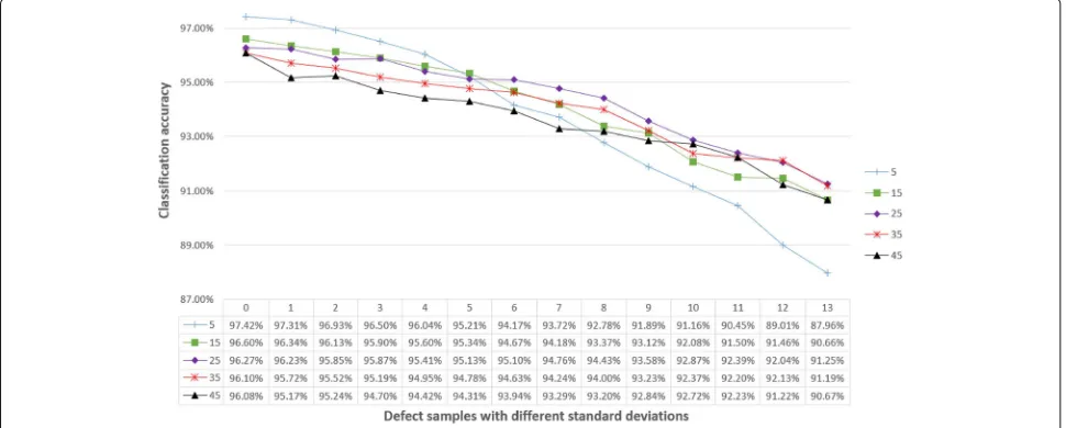
6.3 Number of the sub-SVM classifiers

The number of sub-SVM classifiers, defined ask, is a key parameter for our BYEC classifier. It decides the particle

size to which our system can be adjusted. The purpose of this section is to examine howkaffects the accuracy and the adaptiveness of the BYEC classifier.

We trained five BYEC classifiers with k=5, 15, 25, 35, and 45. These classifiers were trained as described in Section 6.2 with the original defect set, and they were adjusted with 10% of the processed data and tested with 90% of the data set for evaluation. The experimental results are presented in Fig. 9. The highest accuracy on the original defect set is acquired by the classifier with k=5, but the accuracy drops more rapidly compared with the other classifiers that perform at lower accuracy on the defect set with highest noise. The classifier withk = 25 gives the third highest accuracy compared to the original data set but acquires the highest accuracy on the defect set with the highest bias to the original data set. This figure

suggests that the BYEC classifier is more adaptive with a largerk value, but lower accuracy will be achieved with the BYEC classifier on the original data set.

As the results indicate in Fig. 9, k should be set with the real production environment. The BYEC classifier should be set with a largerkvalue when higher adaptive performance is needed. However, to avoid information loss, we should set the BYEC classifier with a smallerk value when the changed model has a small bias with the original model.

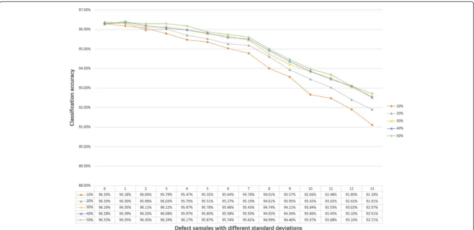
6.4 Set size of the sub-SVM classifiers

An important characteristic of classifiers is the size of the sample set that used to train the classifier. The more sam-ples that are supplied, the more information the classifier machine can learn about the model. For our BYEC clas-sifier, the accuracy of the subclassifiers can be evaluated more precisely with more samples.

The Fig. 10 depicts the accuracy of BYEC classifiers adjusted by different sizes of the samples. All the classifier were performed on the data set described at Section 6.2. We can see that the classifiers trained by 10% reach a low-est accuracy and have least adaptive, but the classifiers trained by 30% reached fairly good performance that the classifiers with more samples adjusted have little advan-tage over this classifier on accuracy and adaptive. Even in the defect set with standard deviation 13, the gap between the BYEC classifier trained by 10 and 50% is 1.01%. This illustrated that our BYEC converged very fast and the low requirement for the sample size.

Figure 10 depicts the accuracy of BYEC classifiers adjusted by different sizes of the samples. All the classi-fiers were used on the data set described in Section 6.2. We can see that the classifiers trained by 10% reach the lowest accuracy and are the least adaptive, but the clas-sifiers trained by 30% reach fairly good performance and classifiers with more samples adjusted have little advan-tage over this classifier in terms of accuracy and adap-tiveness. Even in the defect set with a standard deviation of 13%, the gap between the BYEC classifier trained by 10% and that trained by 50% is only 1.01%. This illustrates that our BYEC classifier converged very fast and the low requirement for sample size.

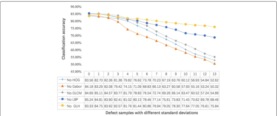
6.5 Evaluating the effect of features

The five types of features selected are able to capture the properties of texture, color, and shape, respectively. Those features are described in detail by Neogi and proved to be very important for classifying steel defects [1]. To evaluate the effect of each feature, when the num-ber of features is less than four, we observe that the accuracy of our method dropped very significantly, with accuracy barely reaching 70%. Therefore, we discuss the meaningful situation in which four features are used to classify the steel.

The Fig. 11 shows the accuracy of EFIC classifiers adjusted by different features. All the classifiers were used on the data set described at Section 6.2.

As shown in Fig. 11, the accuracy of EFIC classifiers without the Gabor feature is the lowest. However, the

Fig. 11The accuracy of BYEC classifiers adjusted by different features on the defect samples with standard deviations₍0₋13₎

Gabor feature is the most suitable for texture representa-tion and discriminarepresenta-tion of steel defect classificarepresenta-tion.

In contrast, the accuracy of EFIC classifiers without GLH is the highest. This demonstrates that the GLH fea-ture is the least suitable for steel defect classification. The main reason for this is that the GLH feature can only cap-ture gray feacap-tures but not texcap-ture and or shape. Other good performance features followed by four features no HOG, GLCM, and LBP.

In conclusion, in our experiments, the absence of any one feature of EFIC classifiers significantly reduced the accuracy. Therefore, by combining these five features, our method can obtain satisfactory accuracy for steel defect classification.

7 Conclusions

Because accuracy decreases in steel surface classifica-tion systems with a changed producclassifica-tion line model, in this research, we propose an evolutionary method that can be adjusted with a small sample set to fit a changed model and maintain relatively high accuracy. First, to overcome information loss in the process of evolution, we proposed five kinds of features that cover texture, color, and shape, respectively. Second, random subspace SVM classifiers are proposed to conquer the overfitting prob-lem and fit for adjustment. Then, we introduced a naive Bayes machine to fuse the results from SVM subclassi-fiers that suits the adjustment and requires a small sample set. Finally, we introduced a simple method to adjust the Bayes kernel. The experimental results indicate that the BYEC algorithm is more adaptive with changed steel sur-face defect data set compared with other algorithms. Our

research suggests that the adaptiveness of the classifier is highly related to the parameterk; with the growth ofk, the BYEC classifier shows a greater adaptiveness but, unfor-tunately, with some accuracy loss on the original data set. The small sample set requirement was shown to have been fulfilled from the experiment results.

With the advantages and disadvantages of the BYEC algorithm, in a new production line, we can use the orig-inal BYEC algorithm without any labeled samples on the changed model; with the growth of the sample set size, we can adjust the BYEC model to become more adaptive. A new classifier can be trained to replace the old classifier as the relatively low accuracy on large sample set. Our future work will focus on increasing the accuracy on both a large sample set and a changed production model. Meanwhile, more noise-robust methods can be combined with this method to increase the adaptiveness.

Endnote

1_{NEU surface defect database is the the Northeastern}

University (NEU) surface defect database, download link: http://faculty.neu.edu.cn/yunhyan/NEU_surface_defect_ database.html.

Acknowledgements

We thank Dr. Qiaochuan cheng from the Department of Electronics and Information Engineering, Tongji University, and anonymous reviewers for their useful comments and language editing which have greatly improved the manuscript.

Funding

Authors’ contributions

MX and MJ conceived and designed the study. MX, MJ, LX, and LY performed the experiments. MX and MJ wrote the paper. GL, MX, MJ, LX, and LY reviewed and edited the manuscript. All authors read and approved the manuscript.

Competing interests

The authors declare that they have no competing interests.

Publisher’s Note

Springer Nature remains neutral with regard to jurisdictional claims in published maps and institutional affiliations.

Author details

1_{School of Computer Science and Information Engineering, Shanghai Institute}

of Technology, Shanghai, China.2Department of Electronics and Information Engineering, Tongji University, Shanghai, China.

Received: 29 February 2016 Accepted: 4 July 2017

References

1. N Neogi, DK Mohanta, PK Dutta, Review of vision-based steel surface inspection systems. EURASIP J Image Video Process.2014(1), 1–19 (2014) 2. F Dupont, C Odet, M Cartont, Optimization of the recognition of defects

in flat steel products with the cost matrices theory. NDT & E International.

30(1), 3–10 (1997)

3. C Unsalan, A Erci,Automated inspection of steel structures. Recent Advances in Mechatronics. (Springer-Verlag Ltd, Singapore, 1999), pp. 468–480 4. S Ghorai, A Mukherjee, M Gangadaran, PK Dutta, Automatic defect

detection on hot-rolled flat steel products. IEEE Trans. Instrum. Meas.

62(3), 612–621 (2013). doi: 10.1109/TIM.2012.2218677

5. X-Y Wu, K Xu, J-W Xu, inImage and Signal Processing, 2008. CISP’08. Congress on. Application of undecimated wavelet transform to surface defect detection of hot rolled steel plates, vol. 4 (IEEE, 2008), pp. 528–532. http://ieeexplore.ieee.org/document/4566708/

6. K Song, Y Yan, A noise robust method based on completed local binary patterns for hot-rolled steel strip surface defects. Appl. Surface Sci.285, 858–864 (2013)

7. C Yan, Y Zhang, J Xu, F Dai, L Li, Q Dai, F Wu, A highly parallel framework for HEVC coding unit partitioning tree decision on many-core processors. IEEE Signal Process. Lett.21(5), 573–576 (2014)

8. G Wu, H Kwak, S Jang, K Xu, J Xu, inAutomation and Logistics, 2008 ICAL 2008. IEEE International Conference on. Design of online surface inspection system of hot rolled strips (IEEE, 2008), pp. 2291–2295. http://ieeexplore. ieee.org/document/4636548/

9. Y-J Liu, J-Y Kong, X-D Wang, F-Z Jiang, inAdvanced Computer Theory and Engineering (ICACTE) 2010 3rd International Conference on. Research on image acquisition of automatic surface vision inspection systems for steel sheet, vol. 6 (IEEE, 2010), pp. V6–189. http://ieeexplore.ieee.org/ document/5579393/

10. M Muehlemann,Standardizing defect detection for the surface inspection of large web steel. (Illumination Technologies Inc, 2000), pp. 1–9. http://www. il-photonics.com/cdv2/Illumination%20tech-Light%20Sources/white %20papers/surface_inspection.PDF

11. T Ojala, M Pietikäinen, T Mäenpää, Multiresolution gray-scale and rotation invariant texture classification with local binary patterns. IEEE Trans. Pattern Anal. Mach. Intell.24(7), 971–987 (2002)

12. RM Haralick, K Shanmugam, IH Dinstein, Textural features for image classification. IEEE Trans. Syst. Man Cybern, (6), 610–621 (1973). http:// ieeexplore.ieee.org/document/4309314/

13. VN Vapnik, V Vapnik,Statistical learning theory, vol. 1. (Wiley, New York, 1998) 14. M Wo´zniak, M Graña, E Corchado, A survey of multiple classifier systems

as hybrid systems. Inf. Fusion.16, 3–17 (2014)

15. JZ Kolter, M Maloof, et al., inData Mining, 2003. ICDM 2003. Third IEEE International Conference on. Dynamic weighted majority: a new ensemble method for tracking concept drift (IEEE, 2003), pp. 123–130. http:// ieeexplore.ieee.org/document/1250911/

16. N Dalal, B Triggs, inComputer Vision and Pattern Recognition, 2005. CVPR 2005. IEEE Computer Society Conference on. Histograms of oriented gradients for human detection, vol. 1 (IEEE, 2005), pp. 886–893. http:// ieeexplore.ieee.org/document/1467360/

17. JJ Henriksen,3d surface tracking and approximation using gabor filters. (South Denmark University, 2007). https://www.yumpu.com/en/ document/view/44234347/3d-surface-tracking-and-approximation-using-gabor-filters-covil

18. UH-G Kreßel, inAdvances in kernel methods. Pairwise classification and support vector machines (MIT Press, 1999), pp. 255–268. http://dl.acm. org/citation.cfm?id=299108

19. C-W Hsu, C-J Lin, A comparison of methods for multiclass support vector machines. IEEE Trans. Neural Netw.13(2), 415–425 (2002)

20. C Cortes, V Vapnik, Support-vector networks. Mach. Learn.20(3), 273–297 (1995)

21. M Göksedef, ¸S Gündüz-Ö ˘güdücü, Combination of web page recommender systems. Expert Syst. Appl.37(4), 2911–2922 (2010) 22. C Porcel, A Tejeda-Lorente, M Martínez, E Herrera-Viedma, A hybrid

recommender system for the selective dissemination of research resources in a technology transfer office. Inf. Sci.184(1), 1–19 (2012) 23. C Cabral, M Silveira, P Figueiredo, Decoding visual brain states from fMRI

using an ensemble of classifiers. Pattern Recognit.45(6), 2064–2074 (2012) 24. M Vangelis, L Androutsopoulos, P Georgios, inCEAS 2006 Third Conference

on Email and AntiSpam (CEAS 2006). Spam filtering with naive bayes-which naive bayes? (Mountain View, 2006). www2.aueb.gr/users/ion/docs/ ceas2006_paper.pdf

25. Y-J Jeon, D-C Choi, JP Yun, C Park, SW Kim, inControl, Automation and Systems (ICCAS) 2011 11th International Conference on. Detection of scratch defects on slab surface (IEEE, 2011), pp. 1274–1278. http://ieeexplore.ieee. org/document/6106307/

26. M Yazdchi, M Yazdi, AG Mahyari, inDigital Image Processing, 2009 International Conference on. Steel surface defect detection using texture segmentation based on multifractal dimension (IEEE, 2009), pp. 346–350. http://ieeexplore.ieee.org/document/5190595/

27. RC Gonzalez,Digital image processing. (Pearson Education, India, 2009). http://web.ipac.caltech.edu/staff/fmasci/home/astro_refs/