1
Vehicle Stabilization via a Self-Tuning Optimal Controller
M. Bayani i*; R. Kazemi ii and Sh. Azadiiii
Received 17September 2007; received in revised 23,September 2009; accepted 28June 2011
i * Corresponding Author, 1Mohsen Bayani Khaknejad awarded MSc in Mechanical Engineering by K. N. Toosi university of technology and is with the Automotive Industries Research and Innovation Center of Saipa, Tehran, Iran (e-mail: [email protected]).
ii R. Kazemi is the Associated Prof. in the Department of Mechanical Engineering, K. N. Toosi University of Technology, Tehran, Iran (e-mail: [email protected]).
iii Sh. Azadi is the Assistant Prof. in the Department of Mechanical Engineering, K. N. Toosi University of Technology, Tehran, Iran (e-mail: [email protected]).
ABSTRACT
Nowadays, using advanced vehicle control and safety systems in vehicles is growing rapidly. In this
regard, in recent years new control systems, called VDC, have been introduced. These systems stabilize vehicle yaw motion, by yaw moment resulted from tire controlling forces. In this paper, an adaptive optimal controller applied to a vehicle to obtain a satisfactory lateral and yaw stability. To derive the control law, we use LQR method. Considering that various parameters are included in the controller structure, which their measurement is either expensive or practically impossible, a least squared estimator with variable forgetting factor is proposed to estimate them. To optimize the system and in order to exert the control yaw moment, an ABS brake system is implemented in a new architecture to distribute brake forces on wheels. The controller rules are derived based on the bicycle model and the estimator is designed based on the 7 DOE model of the vehicle. To simulate and evaluate the performance of the proposed controller the full vehicle model of the reference car in ADAMS/Car, with 214 DOE, is also implemented. Finally, the results of the vehicle response, equipped with the controller system, in a standard maneuver are presented.
KEYWORDS
Vehicle Dynamic Control, ABS, Adaptive Optimal Control, Tire Force Estimation, ADAMS Model.
1. INTRODUCTION
Nowadays, safety is one of the competition factors in auto-industries. Thus we are faced with a progressive implementation of control systems in vehicles; that is due to their great role in prevention of crashes and hazards. It is investigated that the main cause of severe collides, which result in maiming and financial charges, is the spin out of the vehicle about the vertical axis [1]. From vehicle dynamic point of view, this will happen due to excessive side slip and severe over steering.
Lateral stability in ordinary cars is just controlled with the steering input. In critical situations in which vehicle is spinning around the vertical axis rapidly, the dynamic behavior of the vehicle would be nonlinear. This is mainly due to the saturation of tire lateral forces. Research indicates that in critical conditions the lateral dynamic factors don't show a response to the steering input. That is, the car is uncontrollable with the steering input [2].
In recent years, new control systems called VDC are introduced and implemented in modern vehicles. This system will control the yaw behavior of the car by exerting the corrective yaw moment about the vertical axis. This moment is mainly generated by the aim of lateral and longitudinal forces beneath tires. Bearing in mind that lateral tire forces are saturated in critical condition, this will be done by exerting unequal braking or traction forces beneath left and right tires. Considering that most of today cars are equipped with the ABS system, we can take advantage of it for generating the corrective forces. This approach is called differential braking.
benefit an estimator.
One of the first researches deals with vehicle dynamic control is done by Van Zanten and coworkers [1 & 2] the researchers of Bosch company in 1995. They presented their research in the Society of Automotive Engineers conference that could be considered as the birth of the VDC system, by considering all practical and implemental aspects. The structure of the proposed controller was a multi layer system in which the layers operate based on the state feedback and PID controller. Abe and co workers in 2001, analyzed vehicle lateral behavior with vehicle side slip controlling [3]. The control method used was the sliding mode control theorem. The final result of this research is the better performance of the direct yaw moment control system compared with a Four Wheel Steering system (4WS). Chung and Yi in 2006 designed a control system based on the sliding mode theorem to improve vehicle yaw stability [4]. In this research, vehicle instability boundaries are defined according to the side slip angle and its derivation and the control system will be active in case of exceeding from these boundaries. There are also significant researches on identification of tire parameters. One can refer to the work done in 1993 by Huang and coworkers [5] to identify and estimate vehicle parameters using a gradient method. In 2003, Carlson and Gerdes published an article [6] in which they used a non-linear estimator to identify the effective radius of tire and its longitudinal slip coefficient via a nonlinear estimator. Tonelli and coworkers in 2006 estimated the maximum tire friction coefficient in contact with road surface. They evaluated the proposed method performance in condition that the tire slips or purely rotates [7]. Gebbi and coworkers in 2008 designed a six channel sensor with which accurate measurement of tire forces, to be used in VDC systems, would be possible. The important note is considering the price and capability for manufacturing when tackling such equipments [8]. Li and coworkers in 2008 introduced a new algorithm for estimation of tire forces. The simulator they used was a hardware in the loop system with which the robustness of the system is examined in different road conditions [9].
2. MODELING AND VALIDATION
Due to restrictions in controller design based on the mathematical model, we have used the linearized bicycle model with longitudinal, lateral, Yaw DOFs [10], which is depicted in Fig. 1.
Figure 1: Bicycle model.
To use vehicle dynamic equations of the bicycle model in deriving the optimal controller gain, we will linearize the equations by assuming that vehicle speed in small intervals is constant. Undoubtedly, velocity of car in each step of the solution procedure will be updated. By considering that the steering input is small and assuming the steady state condition, the following 2-DOF equations of car are obtained.
(1) r f r f r yf C
F , = 2 α,
α
,(2)
u r L
v fr
r f r f , , , ± − =δ α (3) δ α α α α α f r f r r f f C v u C C r u L C L C mu v
m 2 2 2 2 ⎥ =2
⎦ ⎤ ⎢ ⎣ ⎡ + + ⎥ ⎦ ⎤ ⎢ ⎣ ⎡ − + + z f f r r f f r r f f zz M C L v u L C L C r u L C L C r I + = ⎥ ⎦ ⎤ ⎢ ⎣ ⎡ − + ⎥ ⎥ ⎦ ⎤ ⎢ ⎢ ⎣ ⎡ + + δ α α α α α 2 2 2 2
2 2 2
Here, Mz is the controlling moment. These equations can be represented in the state space form as:
(4)
ED BU AX X= + +
⎥ ⎦ ⎤ ⎢ ⎣ ⎡ = r v
X , U=
[ ]
Mz , D=[ ]
δ, 22 21 12 11 ⎥ ⎦ ⎤ ⎢ ⎣ ⎡ = a a a a
A 10 ,
⎥ ⎥ ⎦ ⎤ ⎢ ⎢ ⎣ ⎡ = zz I B ⎥ ⎥ ⎥ ⎥ ⎦ ⎤ ⎢ ⎢ ⎢ ⎢ ⎣ ⎡ = zz f f f I C Lm C E α α 2 2 mu C C
a =−2 αr+ αf
11 , mu u
C L C L
a =2 r αr− f αf −
12 u I C L C L a zz f f r
r α − α
=2
21 ,
u I C L C L a zz f f r
r α α
2 2 22 2 + − =
In order to simulate the vehicle behavior and evaluate the performance of the proposed controller in the virtual space, we use the 214-DOF full car model in ADAMS/Car. The model used here represents a sedan car equipped with McPherson suspension in front and torsion beam axel in rear. Sub-systems of the ADAMS model and their DOF are given in the Table 1:
TABLE 1
DOF OF ADAMSMODEL SUBSYSTEMS
Sub-System DOF
Front Suspension Assembly with Anti-Roll Bar and Tires 62
Rear Suspension Assembly with Anti-Roll Bar and Rear Tire 116
Steering Sub-System 8
Power Train with Engine Block and Front Differential 22
Car Body 6
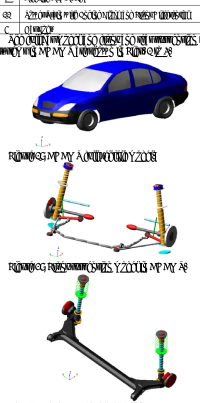
The full car model and front and rear suspension sub-systems in ADAMS are shown in Figs. 2 to 4.
Figure 2: ADAMS full vehicle model.
Figure 3: Front suspension model in ADAMS.
Figure 4: Rear suspension model in ADAMS.
The handling behavior of this model is validated with real test data of the reference car [11], which is given in Figs 5 - 6:
Figure 5: Steering angle vs lateral acceleration in CRC maneuver.
Figure 6: Roll angle vs lateral acceleration in CRC maneuver.
3. CONTROLLER DESIGN
In this section, we will design the control system to derive the controlling yaw moment and consequently, the desired brake torques. To do this, we will make use of the optimal LQR theory. The operation of this system is depicted in Fig 8, for special cases. In the case (a), the vehicle is under steer. Here, the control system guides the vehicle to the desired pass, by exerting the braking force on the rear inner wheel. In case (b) the vehicle is over steer and to guide the vehicle to the desired pass, the controller exerts braking force to the front outer wheel.
As described before a two layer controller is implemented to achieve the stabilization of the car. Different components of the controller and identifier are depicted in Fig 8.
Figure 8: Closed loop diagram of the controlling system.
A. Criterion for Vehicle Dynamic Evaluation
One of the main criteria for vehicle handling evaluation is monitoring the error between vehicle yaw rate and its desired value. The desired yaw rate is calculated in the steady state condition. Consequently, the variation related to the time is assumed to be zero. With this assumption, (3) can be rewritten as a series algebraic relations. With solving these new algebraic equations, the desired yaw rate becomes as (5):
(5)
(
1 Ku2)
Lu r
u d
+
= δ
In which L is equal to Lr+Lf and Ku is the
under-steering coefficient and is calculated as:
(6)
(
)
2
2C C L
C L C L m K
r f
f f r r u
α α
α
α −
=
B. Deriving the Controller Law
For simplification and to reduce the calculation time we use the linear quadratic regulator theory. This will also yield an optimized controlling input which in turn leads to a less energy consumption [12]. Accordingly, we define the controller input as a function of feed-back signals of vehicle dynamic quantities, such as yaw rate, r, lateral velocity, v and feed-forward of the steering input,
δ,.as:
(7)
) ( ) ( ) ( ) ( ) ( ) ( )
(t K t rt K t vt K t t
Mz = r × + v × + δ ×δ
Where, Ki is the controller gain.
Based on the classical optimal control problems we
should define a performance function to optimize the system response. Refer to the importance role of the car yaw rate and lateral velocity in evaluation of the overall lateral dynamic response of the vehicle, we opt these factors to form the performance index as:
(8)
[
]
∫
+ − −= tf
t d
T d T
CF U RU X X Q X X dt
I
0 ( ) ( )
2 1
⎥ ⎦ ⎤ ⎢ ⎣ ⎡ =
2 1
0 0
q q
Q
,
R=[ ]R,
⎥⎦ ⎤ ⎢ ⎣ ⎡ =
r v
X
,
⎥⎦ ⎤ ⎢ ⎣ ⎡ =
d
d r
X 0
,
z
M U=
Q is a positive semi-definite real matrix and R is a definite real matrix. Controller impute is involved in the equation to represent our desire to minimize the consumed energy.
Kalman [12] demonstrated that the optimal answer which satisfies (9) can be presented as the result of the (9) to (11):
(9)
[
() () ()]
) ( ) ( )
(t R1t B t Kt X t St
U =− − T +
(10)
K B KBR Q KA K A t
K()=− T − − + −1 T
(11)
KED QX S B KBR A t
S()=(− T+ −1 T) + d−
In which K is a symmetric 2×2 matrix and contains back gains and S is a 2×1 vector and is the feed-forward portion of the control law. Equation (10) is called as Riccati equation. Regarding to the intense inclination of the controller gains to constant values and considering that using differential equations instead of algebraic equations will complicate both the design and implementation in hardware and software procedures, one can rewrite controller equations as algebraic relations with the assumption of constant control gains in small time intervals.
(12)
0
1 =
− +
+KA Q KBR−B K
K
AT T
(13)
0 )
(−A +KBR−1B S+QX −KED=
d T T
To solve (12) and (13) we use LQ3 theory. Accordingly, the 2n×2n Hamiltonian matrix is defined such that the first n eigen values would be obtained from the matrix of the closed loop system of A-BR-1BTK and
the remaining n eigen values would be obtained as λj(n+i)
= -λji. Hence, matrix of K is calculated by solving the
matrix of equations of the eigen vectors [13].
By choosing R and Q properly we can be assured that optimal results will be gained. One of the approaches to opt appropriate values for R and Q is to assume them as diagonal matrixes consisting of maximum values of state variables and control inputs as their diagonal elements, respectively. That is to choose the elements of these matrixes as ||Xi,Max||2 and ||Ui,Max||2. This method was
(14)
( )
( )
2, 2 22 12
Max z zz z
M I
s r k v k t M t U
× + + = =
C. Brake Force Distribution and ABS Design
In this section, the calculated controller yaw moment in the previous section will be distributed among wheels by exerting brake forces on them.
The designed ABS system operates based on regulating the longitudinal slip of tires in the limits between 0.1 and 0.15. While driver brakes in this domain the maximum possible braking force can be achieved beneath the tires (Fig. 9).
Figure 9: Tire Lateral and longitudinal forces vs slip.
The proposed ABS system operates based on the rules given in Table 2. In each step based on the longitudinal slip of each wheel, the controller regulates the oil pressure in order to exert new brake torques which is the output of the optimal controller in ordinary condition and when the slip is close to the border limits the controller output is the magnitude of the previous step. And if the slip is beyond the border limit brake torque would be 90 percent of the magnitude of the previous step.
TABLE 2
SLIP LIMITS FOR ABSSYSTEM
0 < λ < 0.125 0.125 < λ <0.15
0.15 < λ
Slip Limits
TABS = Tb TABS = Tb-Previous
TABS = 0.9 × Tb-Previous Action
With reference to Fig. (5) and the direction of the vehicle spin about the vertical axis, the wheel on which the control brake torque should be applied is determined. This could simple be done as:
If δ > 0
z r b
z M
T F
M >0⇒ (3)=−2 ×
z f b
z M
T F
M <0⇒ (2)= 2 ×
If δ < 0
z f b
z M
T F
M >0⇒ (1)=− 2 ×
z r b
z F T M
M <0⇒ (4)= 2×
The brake torque to be applied on the nominated wheel is derived based on the wheel dynamic equation
which will be presented in (22) in the next section. If the calculated torque exceeds the boundary limits of that specific wheel, the VDC system will decide to take advantage of other wheels’ baking capacity.
4. ESTIMATOR DESIGN
The basis of the estimation is founded on deriving the unknown parameters based on the available information of the system. One of the most prevalent and basic estimation methods is the least squares (LS) estimation [14]. Usually, to increase the performance of this method, especially when tackling time variable cases, one can take advantage of a coefficient that will decrease exponentially over time. This is to diminish the effect of old data. The main idea in this approach is to minimize the overall error function of (15) with respect to the estimated values, that is
a
ˆ
(
t
)
[15]:(15)
ds
t
a
s
W
s
y
e
J
t rdr
t
s 2
0 ) (
)
(
ˆ
)
(
)
(
−
∫
=
∫
− λThe general mathematical model to relate the unknown parameters to available data can be represented as (16):
(16)
a
t
W
t
y
(
)
=
(
)
Where, a is the vector of unknown parameters, y is the output of the system and W is the matrix of measurable signals. The unknown parameters are iteratively estimated as:
(17)
e
W
t
P
a
ˆ
=
−
(
)
TP(t) is the estimation gain matrix and is written as (18):
(18)
P
t
W
t
PW
P
t
P
dt
d
[
]
=
λ
(
)
−
T(
)
(
)
It is of high importance to mention that to adjust the forgetting coefficient, a greater value of
λ
0 will result in faster estimation as well as more fluctuations in the estimated parameters. This is because of the shortened time to calculate the mean value of the disturbances. Consequently, it is more effective to regulate the value of the forgetting coefficient in the way to have data forgetting when W is always excited permanently. One solution to such a selection can be presumed as (19):(19)
⎟
⎟
⎠
⎞
⎜
⎜
⎝
⎛
−
=
0
0
1
)
(
k
P
t
λ
λ
Where, λ0 and k0 are positive constants, and indicate
maximum forgetting rate and gain matrix upper limit, respectively.
||P(0)|| ≤K0I in order to constrain the gain. In addition,
for the sake of simplification P(0) is defined to be a diagonal matrix as Diag ([5000, 5000, 5000, 5000, 50000000, 50000000, 10000000]) [15].
A. Velocity Estimation and Tire Force identification
In order to calculate the controller moment introduced in (14), we need to have the values of v, u, r, ax, ay, Caf,
Car and δ and to derive the braking torque, values of Fxij
and ωi are needed. Mentioning that measurement of exact velocities of a car is mainly limited due to the high cost of the equipments, we make use of a simplified approach to estimate the lateral and longitudinal velocity.
To estimate vx and vy by using the longitudinal and
lateral acceleration and the yaw angular velocity sensors, we refer to (3) and write the necessary equation as:
(20) ⎥ ⎦ ⎤ ⎢ ⎣ ⎡ + ⎥ ⎦ ⎤ ⎢ ⎣ ⎡ × ⎥ ⎦ ⎤ ⎢ ⎣ ⎡ − = ⎥ ⎦ ⎤ ⎢ ⎣ ⎡ ym xm y x m m y x a a v v r r v v dt d ˆ ˆ 0 0 ˆ ˆ
Where, axm, aym and rm are the measured longitudinal
and lateral accelerations and the yaw angular velocity, respectively.
v
ˆ
xandv
ˆ
yare the estimated longitudinal and lateral velocities.According to equation (1), the lateral forces of tires should be applied in order to calculate the quantities of
Caf and Car. To estimate tire and road interaction forces,
we use least square estimation with exponential forgetting factor. Accordingly, we use 7-DOE equations of car (Fig. 10) with freedom in longitudinal, lateral and yaw direction as well as four degrees of the wheels [11].
Figure 10: Free body diagram of 7 DOF vehicle model. The equations govern this model are given below:
(21)
(
)
( )
[
(
yfl yfr)
( )
xrr xrl]
xfr l f x y x F F Sin F F Cos F F m rv v + + + − + + = δ δ 1
(
)
( )
[
(
yfl yfr)
( )
yrr yrl]
xfr xfl x y F F Cos F F Sin F F m rv v + + + + + + − = δ δ 1
(
)
( )
(
)
( )
[
(
)
(
)
( )
(
)
( ) (
)
⎥ ⎦ ⎤ − + − + − + + − + + + = 2 2 2 1 r xrl xrr f yfr yfl f xfl xfr r yrr yrl f yfr yfl f xfr xfl zz T F F Sin T F F Cos T F F L F F Cos L F F Sin L F F I r δ δ δ δEquation of the wheels’ rotational dynamic is as: (22) 4 , 3 , 2 , 1 , . + − − = −
= F R T T T i
Jiωi xi w bi Rolli
In which, TRoll is the consequence of the hysteresis phenomenon and is called rolling resistance:
(23) 4 , 3 , 2 , 1 , . . =
= f F R i
TRolli r zi wi
fr is the rolling resistance coefficient and for passenger
cars is about 0.01 to 0.02 [10].
Considering that the controller just needs the overall lateral forces for front and rear tires, to reduce the calculation efforts we avoid separating the right and left forces in front and rear axle and assume an overall lateral force for each of the front axles instead of four separated variables. The components of the elements of (17) and (18) are written as:
(24) T w rl rl w rr rr w fl fl w fr fr y x I T w I T w I T w I T w r a a t y ⎥ ⎦ ⎤ ⎢ ⎣ ⎡ − − − − = ) ( (25)
[
]
Tyr yf xrl xrr xfl
xfr F F F F F
F t a()=
(26) ⎥ ⎥ ⎥ ⎥ ⎥ ⎥ ⎥ ⎥ ⎥ ⎥ ⎥ ⎥ ⎥ ⎥ ⎥ ⎥ ⎥ ⎥ ⎦ ⎤ ⎢ ⎢ ⎢ ⎢ ⎢ ⎢ ⎢ ⎢ ⎢ ⎢ ⎢ ⎢ ⎢ ⎢ ⎢ ⎢ ⎢ ⎢ ⎣ ⎡ − − − − − − + − = 0 0 0 0 0 0 0 0 0 0 0 0 0 0 0 0 0 0 0 0 cos 2 2 cos 2 sin cos 2 sin 1 cos 0 0 sin sin 0 sin 1 1 cos cos ) ( w w w w w w w w z r z f z r z r z f f z f f I R I R I R I R I L I L I T I T I T L I T L m m m m m m m m m t W δ δ δ δ δ δ δ δ δ δ δ
5. SIMULATION RESULTS
As indicated before we have made use of ADAMS as an advance solver for simulation and virtual evaluation of vehicle behavior equipped with the proposed controlling system. On the other hand, the designed estimation system has been modeled in MATLAB, which is a powerful calculating and analyzing software. To simulate all these together one needs to establish a direct interconnection between the two software and run them simultaneously.
After developing and validating full vehicle model in ADAMS, we need to build necessary inputs and outputs for the representative of the control system. The needed sensors for this control system are: Body yaw rate sensor, Body longitudinal and lateral accelerations, Steer wheel angle, Wheels angular velocity and Braking torques.
Braking torques applied by the driver
After building the needed sensors and actuators, we should create the control input/output gates and ADAMS/Solver system files which contain the information and equations of the model. Finally, by exporting ADAMS plant model, system files will be implemented in MATLAB/Simulink and the defined input/output channels will form (Fig. 11).
Figure 11: Block diagram of simulator in Matlab/Simulink.
Table 3 illustrates the magnitude of the vehicle parameters used in the model.
TABLE 3 VEHICLE PARAMETERS
Unit Magnitude
Parameter
Kg 1050
m
Kg/m2 1825.2
Izz
m 1.2247
Lf
m 1.4373
Lr
m 1.4375
Tf
m 1.4375
Tr
m/s2 9.806
g
Kg/m2 1.4
Ji
- 0.015
fr
m 0.283
Rw
N 50000
λ
C
N/deg 722.8
α
C
In fact, the simultaneous connection and cooperation of the developed controller in Matlab and the accurate dynamical vehicle model in ADAMS and running the whole in a closed loop is considered as a splendid engineering work.
A. Velocity Estimation and Tire Force Identification
In order to evaluate the performance of the proposed controller, several maneuvers are performed according to ISO standard and prevalent references in auto-industry [11]. Considering the presentation limitations, here we just illustrate and present results of sever braking in lane change maneuver on a µ-split road. In this maneuver driver starts to brake while driving with the initial speed of 100 km/h on a road with different friction coefficients
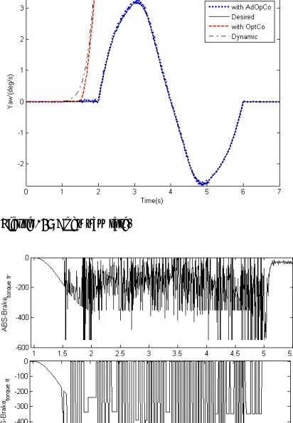
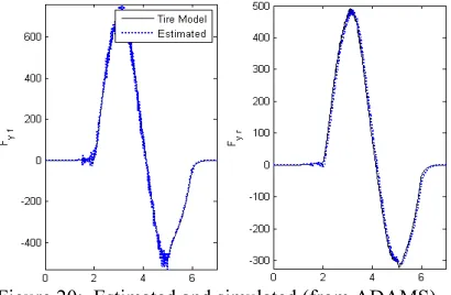
in right and left hand (right: 0.8 and left: 0.3). Furthermore, the driver starts to steer from the second of the maneuver. The steering input and car path is depicted in Fig. 12. All of the presented results with and without the controller are the outputs of full vehicle simulation in ADAMS. Evidently, vehicle without the controller (Dynamic) and the vehicle equipped with the optimal controller and the ABS system (with OptCn) rapidly tend to instability and disobey the driver inputs. On the other hand, the appropriate response of the vehicle equipped with adaptive controller with modified ABS (AdOpCn) is evident. Fig. 15 depicts the accurate response of the adaptive controller to follow the desired yaw rate. The performance of the modified ABS system is also illustrated in Fig. 18. It is crystal clear that the slip is maintained in the target domain. The rapid and precise performance of the velocity estimator and tire force identifier is presented in Figs. 13, 19 and 20. Brake torques applied by the ABS actuators on wheels are presented in Fig. 16 and 17. This periodic actuation from frequency point of view is completely applicable in current ABS systems [16].
Figure 12: Steering wheel angle and vehicle trajectory.
Figure 14: Lateral and longitudinal acceleration of car body.
Figure 15: Body yaw rate.
Figure 16: Brake torques of front wheels applied by the optimal controller.
Figure 17: Brake torques of rear wheels applied by the optimal controller.
Figure 18: Longitudinal tires' slip.
Figure 20: Estimated and simulated (from ADAMS) lateral force of tires.
6. CONCLUSION
In this research, we have designed and proposed an adaptive optimal controller to control and stabilize the lateral and rotational behavior of vehicle by the aim of differential braking concept. Accordingly, we distributed the controller braking forces with a new approach via an ABS system. The parameters of the optimal controller are regulated by an identifier and the velocity of the car is estimated in a simple way. Results of the vehicle maneuvers in standard condition indicate the appropriate performance of the controller.
7. NOMENCLATURE
Earth gravitational acceleration g
Friction coefficient between the tire and road
µ
Vehicle longitudinal velocity vx , u
Vehicle lateral velocity vy , v
Vehicle longitudinal acceleration ax
Vehicle lateral acceleration ay
Rolling resistance coefficient fr
Vehicle yaw rate r
Rotating angular velocity of the wheels ωi
Longitudinal slip of tires λi
Lateral Slip of Tires αi
Vehicle total mass m
Vehicle yaw moment of Inertia Izz
Distance between vehicle CoG from front axle Lf
Distance between vehicle CoG from rear axle Lr
Front tread Tf
Front wheels steer angle
δ
Lateral stiffness of tires Cαi
Longitudinal stiffness of tires Cλi
Tire longitudinal force Fxi
Tire lateral force Fyi
Understeering coefficient Ku
State vector X
State space matrixes A,B,C,E
Wheel moment of inertia Ji
Controlling input U
Disturbance D
Desired state vectors Xd
Desired yaw rate rd
Effective radius of tires Rw
Performance index J
Gain matrix in performance index T,Q,R
Feedback gains Ki
Hamiltonian function H
Wheel traction torque Ti
Wheel braking torque Tbi
Rolling resistance torque
TRoll
System output vector y
Signal matrix W
System unknown parameters estimation vector a
System unknown parameters estimation vector â
8. REFERENCES
[1] A. Van Zanten, R. Erhardt, K. Landesfiend and G. Pfaff, "VDC System development and perspective", in proc. 1998 SAE, paper No. 980235.
[2] A. Van Zanten, R. Erhardt and G. Pfaff "VDC, the Vehicle Dynamics Control System of Bosch", in proc. 1995 SAE, paper No. 950759.
[3] M. Abe et al, "Side-slip control to stabilize vehicle lateral motion by direct yaw moment", in proc. 2001 JSAE Review 22, pp. 413– 419.
[4] T. Chung and K. Yi, "Design and evaluation of side slip angle-based vehicle stability control scheme on a virtual test track", IEEE Trans. on Cont. Sys. Tec., vol. 14, No. 2, pp. 224-234, 2006. [5] F. Huang, J. R. Chen and L. W. Tsai, "The use of random steer test
data for vehicle parameter estimation", in proc. 1993 SAE, paper No.930830.
[6] C. R. Carlson and J. C. Gerdes, "Nonlinear estimation of longitudinal tire slip under several driving conditions", in proc. 2003 American Control Conf., pp. 4975-4980, 2003.
[7] M. Tanelli and M. S. Savaresi, "Friction-curve peak detection by wheel-deceleration measurements", Intelligent Transportation Sys. Conf. IEEE, Vol. 17-20, pp. 1592-1597, 2006.
[8] M. Gobbi, J. Botero and G. Mastinu, "Improving the active safety of road vehicles by sensing forces and moments at the wheels", Veh. Sys. Dyn., Vol. 46, 2008.
[9] L. Li, J. Song, H. Wang and C. Wu, "Fast estimation and compensation of the tyre force in real time control for vehicle dynamic stability control system", Int. Journal of Vehicle Design, Vol. 48, pp. 208-229, 2008.
[10] J. Y. Wong, Theory of Ground Vehicles, John Wiley & Sons Inc., 2001.
[11] M. B. Khaknejad, "Designing Vehicle Dynamic Stabilizer Estimator", MSc dissertation, Dept. Mechanical Eng., Univ. K. N. Toosi, Tehran, 2007.
[12] D. E. Kirk, Optimal Control Theory, Englewood Clifs, Prentice Hall, 1970.
[13] A. Gaffari, Advanced Control Course Book, Tehran, K. N. Toosi Univ. Pub., 2002.
[14] R. Lozano, D. Dimogianopoulos and R. Mahony, "Identification of linear time-varying systems using a modified least-squares algorithm", Journal of Automatica, Vol. 36, pp. 1009-1015, 1999. [15] J. J. Slotine and W. Li, Applied Nonlinear Control, 1st ed., Prentice
Hall International Inc., 1992.