R E S E A R C H
Open Access
Geometric bounding box interpolation:
an alternative for efficient video annotation
Pedro Gil-Jiménez
*, Hilario Gómez-Moreno, Roberto López-Sastre and Saturnino Maldonado-Bascón
Abstract
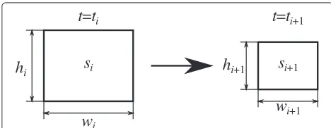
In video annotation, instead of annotating every frame of a trajectory, usually only a sparse set of annotations is provided by the user: typically its endpoints plus some key intermediate frames, interpolating the remaining annotations between these key frames in order to reduce the cost of the video labeling. While a number of video annotation tools have been proposed, some of which are freely available, and bounding box interpolation is mainly based on image processing techniques whose performance is highly dependent on image quality, occlusions, etc. We propose an alternative method to interpolate bounding box annotations, based on cubic splines and the geometric properties of the elements involved, rather than image processing techniques.
The algorithm proposed is compared with other bounding box interpolation methods described in the literature, using a set of selected videos modeling different types of object and camera motion. Experiments show that the accuracy of the interpolated bounding boxes is higher than the accuracy of the other evaluated methods, especially when considering rigid objects. The main goal of this paper is related with the bounding box interpolation step, and we believe that our design can be integrated seamlessly with any annotation tool already developed.
Keywords: Video annotation, Bounding box interpolation, Projective geometry, Cubic splines
1 Introduction
The growth in image and video processing demands larger quantities of annotated training data. A still image can be annotated at different levels. At the image level, annota-tions consist of simply indicating the objects present in the image, without any spatial information. At the pixel level, each pixel must be assigned to a label. Intermediate solutions may consist of drawing polygons surrounding the object or simple geometric shapes, such as rectan-gles or ellipses. The complexity, and thus, the cost or time required to annotate an image, depends on the level at which we need to annotate it.
Large-scale image databases are useful for supervised learning of visual object appearance. There are many pub-licly available databases. For instance, the PASCAL VOC Challenge [1] provides a standard dataset of annotated images at the bounding box level, for object categorization and detection. The images are collected from the flickr photo-sharing web site, and annotations are done at a
*Correspondence: [email protected]
Signal Theory and Communication Department, Universidad de Alcala, Crta Madrid-Barcelona km 33.600, Alcala de Henares, Spain
single annotation “party”, to ensure consistency. The Ima-geNet database [2] offers a collection of tens of millions of annotated images hierarchically organized, in this case, at the image level.
Many applications has been proposed in the literature for the task of image annotation, both for personal use and for massive annotations. In [3], Russell et al. proposed LabelMe, a web-based open tool that allows polygon-based image annotations. This tool can be accessed freely by any researcher, either to annotate their own images or to download the already annotated image collections. In [4], von Ahn and Dabbish took advantage of theGames With A Purpose(GWAP) philosophy to develop an online game which allows image annotation while the users are enjoying the game. In this case, images can only be anno-tated at the image level. The Human Intelligence Task (HIT) service provided byAmazon Mechanical Turkwas explored by Sorokin and Forsyth [5] to outsource human annotation services at a low cost. This approach enables the annotation of large image databases at the bounding box level in a short time.
Video annotation can also be done at different levels. For instance, ANVIL [6] is a free tool that allows video
annotations at the frame level, that is, without any spatial information. However, when object location is required, the temporal evolution of the annotated objects must also be provided. Manually annotating the object location for all the frames in the video sequence is a tedious task. This is typically solved by allowing the user to provide only a limited set of annotations for a given object, then propa-gating this to the rest of the frames. The frames where the annotations are supplied are calledkey frames, and this set must usually include the first and last frames where the object is visible, in order for the system to know the endpoints of the object’s trajectory.
The number of key frames needed depends on many factors, such as the object type (rigid or non-rigid), tra-jectory length (number of frames), type of object motion (straight, curved, or chaotic), and the accuracy required for the propagated annotations. The number and posi-tion of these key frames can be fixed or defined by the user. Vondrick et al. [7] discovered that ‘a fixed key frame schedule is significantly faster than a user-defined key frame schedule.’ However, the key frame frequency needs to be adjusted depending on the type of motion to annotate. When an object moves in a chaotic trajec-tory, more annotations are needed in order to accurately handle the chaotic motion. In this paper, however, we are not concerned with this issue and will use both schedules indiscriminately.
Propagation across frames has typically been performed by means of image and video processing techniques. In [8], Badrinarayanan et al. proposed a propagation scheme, given the pixel-level annotation of the first and last frames of a video sequence. The algorithm is based on a hid-den Markov model and labels every pixel in all the frames between the endpoints. In [9], Liu et al. proposed a con-tour tracker to track the concon-tour provided by the user in the first frame. The user can specify a time-varying depth value for each annotated object, intended to handle occlu-sions and 3D linear interpolation. The user may also be requested for an inspection to correct tracker mistakes. Contour tracking is also used in [10] to track annotated curves in a video sequence forrotoscoping, i.e., the pro-cess of tracking shapes throughout a video sequence. In [11], Kalal et al. proposed a long-term tracker of a bound-ing box provided by the user in the first frame. The system is able to automatically re-detect the object after a period when it is not in the field of view or after tracking fail-ure, by learning the object appearance from the previous frames.
Propagation can also be done by means of the geometric properties of the elements involved. In this case, the user provides a set of simple (rectangle, ellipse, etc.) or complex shapes, and the system computes the coordinates of the polygon for the remaining frames. For this case, the main techniques described in the literature will be analyzed in
Section 2, where different publicly available annotation tools will be introduced. Section 3 describes the alterna-tive procedure proposed in this paper. Section 4 describes the experiments performed to compare the existing soft-ware applications. Section 5 concludes the paper.
2 Related works
In this paper, we propose an alternative method to prop-agate bounding box annotations between key frames. For that reason, we will analyze here the most popular soft-ware packages for video annotation at the bounding box level, focusing on the propagation algorithms proposed in each.
2.1 Available software
VIdeo Performance Evaluation Resource (ViPER) is one of the earliest video annotation tools provided by the research community [12]. The initial goal was to create a flexible ground truth format and a tool for ground truth generation and sharing. It is a JAVA application that allows the user to define object categories (people, cars, ani-mals, etc.) and different attributes, including spatial ones (bounding box, bounding ellipse, points, etc.). The soft-ware includes a default linear interpolation utility. For this interpolator, if we define bi to be the coordinates of a bounding box att=ti, then
bi=
xi yi wi hi
, (1)
where (xi,yi) are the coordinates of the center of the bounding box and(wi,hi)are its width and height. Given two consecutive annotationsbiandbi+1, the coordinates of the bounding box for a given timet=tjare
bj=
ti+1−tj ti+1−ti
bi+
tj−ti ti+1−ti
bi+1. (2)
Linear interpolation can be defined as the simplest approach [7] for label propagation. This method has two main drawbacks. On the one hand, linear interpolation can only handle straight trajectories, since interpola-tion between adjacent segments are computed indepen-dently. On the other hand, it can not accurately capture scale transformations due to perspective effects. A recent update can be found in [13], which allows semiautomatic video annotation. Nevertheless, the system is based on a foreground/background motion detection, which limits its use to videos recorded with static cameras.
being the linear interpolation discussed above. The other method is based on dynamic programming, using a visual model of the annotated object. They extract the model from theN bounding boxes provided, compute a feature descriptor composed of HOG and color features, and train a linear SVM classifier from positive and negative (back-ground) samples. The main drawback is that the algorithm is highly dependent on the image quality, and the system can even fail in the case of object occlusions. The sys-tem includes a constant to allow the visual interpolator to gracefully degrade to linear interpolation when the former becomes inaccurate.
Instead of relying on visual properties, the interpola-tion can be done using the geometric properties of the elements involved. In this case, when interpolating coor-dinates, we can use image or spatial coordinates.
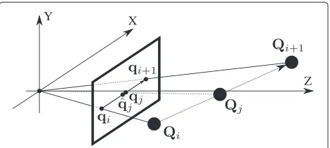
Consider a pointQmoving in front of a camera, as in Fig. 1. Att = ti, the point will be located atQiin spatial coordinates, and its image will be atqi, and similarly for t = ti+1. If we suppose constant motion for the point, at tj = (ti +ti+1)/2, the point will be located atQj, at the intermediate position between the points in space and its image atqj. However, if we interpolate using image coor-dinates, the point qˆj will be located at the intermediate position between the image points, and as can be seen in Fig. 1, the coordinatesqjandqˆjdo not coincide, due to the effects of perspective.
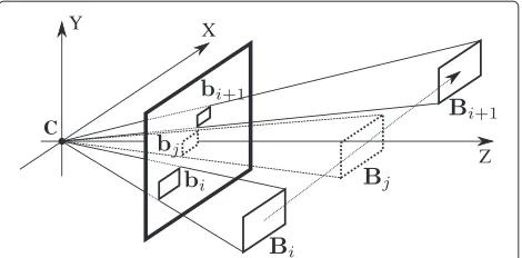
Perspective effects get canceled only when the object moves parallel to the image plane. These effects increase as the component of the motion normal to the image plane increases. For instance, in Fig. 2, we can see two annotated trajectories. Object1moves almost parallel to the image plane, so that the perspective effects are mini-mal and interpolation using image coordinates can be an accurate solution.
However, parallel motion is not the general situation. For object2in Fig. 2, the variation in depth is large. In this situation, the last assumption does not hold, and the accuracy in the bounding box interpolation decreases, as we will see later, in Section 4.
Fig. 1Interpolation of the intermediate position betweenQiand Qi+1using image (qˆj) and spatial (qj) coordinates
Fig. 2Perspective effects for an object which moves parallel (1) and for an object which does not move parallel (2) to the image plane
To take into account this effect, Yuen et al. [14] pointed out that ‘a constant velocity in space does not project to a constant velocity in the image plane, due to perspec-tive effects.’ In their work, they proposed an alternaperspec-tive method to project the coordinates of the annotated object to the image plane for any time between two key frames.
Assuming that an object in space is moving with con-stant motion between two key frames, any point of the object will therefore move in a straight line. The line in the image plane joining the same point of the object in both key frames will be the image of the line followed by this point in space. If all the points of the object move in paral-lel trajectories, all points in space will meet at infinity, and so the cross point in the image plane of all lines will be the vanishing point for this trajectory. The coordinates of any point of the object for a given timetis computed using
(x(t),y(t))=
x0+λ(t)xv
λ(t)+1 ,
y0+λ(t)yv
λ(t)+1
(3)
where (x0,y0) are the coordinates of the point in the frame att = 0, andpv = (xv,yv)are the coordinates of the vanishing point computed as described above.λ(t)is the displacement of the point along the direction of the motion in space, and since constant motion is assumed, we haveλ(t) = vt, wherevis the velocity of the point in space and can be computed, given a second key frame at t=t1, using
v= x1−x0 t1·(xv−x1)
. (4)
Fig. 3Errors in computation of the vanishing point from a pair of bounding boxes
to meet at the same point. For some points in the last figure, some of the cross points are even located outside the image plane. Furthermore, for motion parallel to the image plane, the vanishing point will lie at infinity, so that in (3), there is an indetermination that must be resolved some other way. The second drawback is that this schema can only be employed between a pair of key frames, while assuming straight paths in between, which is not a correct assumption for object motion in general.
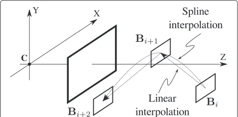
The second drawback is solved by Lee et al. in [15, 16] by interpolation using cubic splines [17]. In their work, they proposed a tool for collaborative video annotation, mainly intended for interactive services (i.e., smart TV) in the multimedia industry. They also proposed a dynamic sampling-based cubic spline interpolation (DSCSI) algo-rithm to reduce the size of the trajectory data on a “clickable video”. Focusing on the interpolation part, the object position is computed using cubic spline interpola-tion (CSI) from a sparse set of annotainterpola-tions. Nevertheless, the interpolation is performed using image coordinates instead of spatial coordinates, so that, as explained above, it is not able to accurately model object trajectories with large depth variations.
To address these problems, in this paper, a new inter-polation algorithm that combines a 3D reconstruction schema is proposed, similar to the one proposed in [14], with the cubic spline interpolation used in [16]. How-ever, the main difference with respect to [14] is that the algorithm proposed in our paper performs a con-tinuous reconstruction in the spatial coordinates, as will be described in Section 3.3. This improvement allows us to use cubic splines to interpolate the spatial bound-ing box coordinates, instead of usbound-ing linear interpolation, to model object trajectories. The main difference with respect to [16] is that the proposed 3D reconstruction allows us to model more accurately the trajectory of objects when they exhibit large depth variations.
3 Geometric interpolation
In this section, we will describe the process designed to compute the bounding box coordinates for any frame
from the known bounding box annotations. The over-all schema is depicted in Fig. 4. Suppose we have two annotationsbiandbi+1of an object, the key idea is find-ing the coordinates Bi andBi+1of the bounding box in space. Having that, computing the coordinatesbj of the bounding box in the image plane for any timet = tj is straightforward, assuming we know the motion model of the object in space.
We will demonstrate that using only bounding box coordinates, we can perform a 3D reconstruction of the bounding box positions. If the camera’s internal param-eters are not known, i.e., we are working with an uncal-ibrated camera, the 3D positions can be computed only up to a scale transformation. Nevertheless, we will see that actual 3D coordinates are irrelevant for bounding box interpolation, and so, no camera calibration is needed.
Prior to defining the interpolation schema proposed in this paper, we introduce briefly the basic concepts related with central projection and the camera model needed. The notation has been taken from [18] where possible. We will first describe the interpolation technique for a sim-pler two-dimensional case and then extend the concepts to three dimensions.
3.1 Two-dimensional camera model
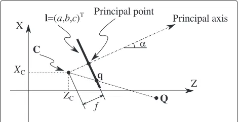
In the two-dimensional case, central projection is based on theline camerashown in Fig. 5. This camera projects points on the plane XZonto animage line. Let the cen-ter of projection be the pointC=(XC,ZC, 1)T, expressed in homogeneous coordinates, and letl =(a,b,c)Tbe the homogeneous vector representing the image line. The dis-tance from the linelto the pointCisf, which is called the focal lengthof the camera. The line from the center of pro-jection, normal to the image line, is called the principal axis of the camera, and the cross point between the image line and the principal axis is called the principal point.
Fig. 4Overview of 3D interpolation technique. Given annotationsbi
andbi+1, the computation ofbjis performed by a 3D reconstruction
Fig. 5Model for a two-dimensional projective camera
Under this model, a point Q = (XQ,ZQ, 1)T in the plane is mapped to the pointq = (xq,wq)T in homoge-neous coordinates in the image line. This point will be located where a line joining the pointQwith the center of projectionCmeets the image line. The homogeneous coordinates of q can be computed from the projection matrixP:
P=K·R·[ I| −C] (5)
where K is the 2×2 camerainternal parametermatrix, R is the 2 × 2 camera rotation matrix, I is the 2× 2 identity matrix, andC= {XC,ZC}is the center of projec-tion expressed in inhomogeneous coordinates. In order to simplify the problem, suppose that the camera is placed at a canonical position, that is, suppose that the cen-ter of projection is the origin of the coordinate system, C = (0, 0, 1)T, and that the principal axis is the Z axis (α=0), as in Fig. 6. Furthermore, we can have the princi-pal point be the origin of the image coordinate system. In this situation, P reduces to
P=
f 0 0 1
·
1 0 0 1
·
1 0 0 0 1 0
=
f 0 0 0 1 0
. (6)
A pointQ=XQ,ZQ, 1
T
in the plane is projected onto the image line at
Fig. 6An object moving in the planeXZ, with the camera placed at a canonical position
q=
xq wq
=P·Q=
f ·XQ ZQ
(7)
which can be expressed in inhomogeneous coordinates as
q= f ·XQ ZQ
. (8)
3.2 Reconstruction for a single segment
Now, consider an object moving in front of a line camera fromt=titot=ti+1, as shown in Fig. 6. In this section, we will consider a trajectory defined by only one segment, that is, only two key frames, at the start and endpoints of the trajectory, without intermediate key frames. In the fol-lowing sections, we will extend the method to any number of segments.
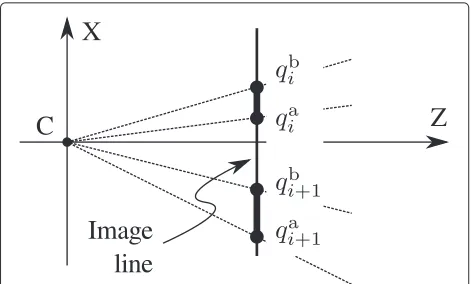
If we call a the lower edge of the object, and b the upper one, as can be seen in Fig. 7, the edges of the object will have inhomogeneous coordinatesQai = {Xai,Zi}and
Qbi = {Xbi,Zi}, respectively. Note that we have assumed the object to be parallel to the image line, thus the coordi-nateZfor both points is the same. Under a camera matrix P, the pointais imaged onto the image line at
qai = f ·X a i Zi
(9)
as shown in Fig. 8. If the shift of the object fromtitoti+1 isi = {Xi,Zi}, then the coordinates for point aat t=ti+1will be
Qai+1=Qai +i (10) and will be imaged by the camera at
qai+1= f ·(X a i +Xi)
Zi+Zi (11)
and similarly for pointb. Gathering all the equations, we have
⎧ ⎪ ⎪ ⎪ ⎪ ⎪ ⎪ ⎨ ⎪ ⎪ ⎪ ⎪ ⎪ ⎪ ⎩
qai = f·Xia Zi
qbi = f·Xbi Zi
qai+1= f·(Xia+Xi) Zi+Zi
qbi+1= f·
Xbi+Xi
Zi+Zi .
(12)
Fig. 8Projection of the object points onto the camera image line
Before going on, we will analyze the effect of the focal lengthf. As can be seen in Fig. 9, for an image pointqiat t=ti, if we assume the point depth to beZ=Ziand use a camera with focal lengthf, the point is back projected to
Qi = {Xi,Zi}. Now, changing the camera focal length to f=kE·f while keeping the same depthZi, the point coor-dinates will change toQi = {Xi,Zi}. By similar triangles, we have
qi f =
Xi Zi
(13)
and
qi f =
Xi Zi
(14)
which gives Xi = kE ·Xi, and the same for t = ti+1. Since our final interest is not the reconstruction itself, but the computation of the images of intermediate positions, it can easily be seen that the interpolation is indepen-dent of the particular focal length chosen. For instance, if we interpolate the image coordinates for the point at the middle position between ti andti+1, assuming constant
Fig. 9Effect of the camera focal length on the interpolated points. The inhomogeneous coordinateqjof the interpolated point is
independent of the particular focal lengthfchosen
motion, the coordinates for the point when focal length is f will be
Qj=
Xi+Xi+1
2 ,
Zi+Zi+1 2
(15)
which will be imaged at
qj=f
Xi+Xi+1 Zi+Zi+1
. (16)
In the same way, if the focal length isf, the interpolated position will be
qj=f
Xi+Xi+1 Zi+Zi+1
=f
Xi+Xi+1 kE·(Zi+Zi+1)
=qj,
(17)
that is, both points are imaged onto the same image coordinate. Figure 9 shows a graphical example.
The last proof shows that the coordinate of the interpo-lated points is independent of the particular focal length chosen, and therefore, the internal camera parameters are not needed. Thus, to simplify the problem, we choose f =1. Reorganizing the initial equations,
⎧ ⎪ ⎪ ⎨ ⎪ ⎪ ⎩
qaiZi−Xia=0
qbiZi−Xib=0
qai+1Zi+qai+1Zi−Xia−Xi=0
qbi+1Zi+qbi+1Zi−Xib−Xi=0
. (18)
The last result forms a system of linear equations in the unknownsBi=[Xai,Xbi,Zi,Xi,Zi], which can be com-puted from its null space. Since (18) is a homogeneous system of equations, Bi can be found up to a constant factorks. The meaning from the geometric point of view is that the space is reconstructed up a scale transfor-mation. However, under central projection, two points related by a scale transformation are imaged onto the same image coordinates. This means that the particular constant factor ks chosen for Bi is not important, since only the relation between all variables is important. We will come back to this concept when analyzing trajectories composed of more than one segment.
With a little computation from (18), we get
qai+1−qaiZi+qia+1Zi−Xi=0
qbi+1−qbiZi+qbi+1Zi−Xi=0 (19) and
Xia=qaiZi
Xib=qbiZi . (20)
Solving (19) using the cross product, we obtain
⎧ ⎨ ⎩
Zi=qib+1−qai+1=si+1
Zi=
qbi −qia−qbi+1−qai+1=si−si+1
Xi=qbiqai+1−qaiqbi+1
wheres =qb−qa is the size of the object in the image line. Finally, (20) can be solved using these last results:
Xia=qai ·si+1
Xib=qbi ·si+1 . (22)
3.3 Reconstruction from multiple segments
The results obtained in the previous section allow us to interpolate the coordinates for any frame between two key frames. For a trajectory composed ofN key frames, we could apply the same process independently for the N − 1 segments. However, since the computations are independent, the results would give disjoint reconstructed segments. To see this, suppose we have three different annotations for an object,bi,bi+1, andbi+2, as in Fig. 10.
The reconstruction for the segment defined bybi and
bi+1givesBiandBi+1. Likewise, for pointsbi+1andbi+2 we haveBi+1andBi+2. The reconstructed segments will be, in general, disjoint. Although both reconstructions are correct, they are only useful if further interpolations are performed independently for each segment, i.e. assum-ing straight paths between key frames. However, typi-cal object motion is better modeled with interpolation schemes which need more samples. As we will see later, we will use cubic spline interpolation, a method which uses more than two samples to compute any interpolation. To this end, we need the reconstructed trajectory to be continuous along the whole path.
Continuity can be achieved easily taking into account that reconstruction can only be computed up to a scale transformation. We can adjust the scale factorks, intro-duced before, for the second segment to haveBˆi+1=Bi+1:
ˆ
Bi+1=ksi ·Bi+1=Bi+1 (23)
wherekis = Zi+1/Zi+1is the scale factor to be applied to the second segment, that is,Bˆi+1 =kis·Bi+1andBˆi+2=
ksi ·Bi+2. Figure 11 shows how, applying this scale correc-tion, we can make the trajectory continuous. Furthermore, for the next segment, a new scale factorkis+1=Zi+2/Zi+2
Fig. 10Independent reconstruction for two segments of an object trajectory
Fig. 11Scale correction for the second segment to build a continuous trajectory
must be computed, so that the coordinates for that seg-ment will beBˆi+2 = kis·kis+1·Bi+2 = kis·Bi+2, and so on.
3.4 Three-dimensional case
Extrapolating the problem to three dimensions is not straightforward. A first approach could be to perform the reconstruction independently for the horizontal and verti-cal coordinates, but this would yield different depth values (Zi andZi) for the horizontal and vertical reconstruc-tions. Although we can adjust the scale factorks of one of the coordinates to make the depth valuesZiequal for both coordinates, the other value, Zi, will, in general, be different and so will be the object depth fort = ti+1, but, obviously, the depth position should be the same for both coordinates along the whole path, since it is the same point.
The depth values for the horizontal and vertical coor-dinates will only be equal when the bounding box aspect ratio is kept constant between annotations. Thus, to improve the performance, we have to correct the aspect ratio variation between key frames. To see this, suppose given an object annotation fort = tiandt = ti+1as in Fig. 12. As the object moves away from the camera, its size will decrease and inversely. If the aspect ratio of the anno-tated rectangle was kept constant between the key frames, this would be the only variation on both height and width. This can easily be checked if we look at the equations in (21) for the computation of Z andZ. Applying the
equation for the computation of the depth information, substituting s → w for the horizontal coordinate, and s→hfor the vertical coordinate, we haveZix =wi+1and
Zix = wi −wi+1for the x coordinate andZyi = hi+1 andZiy = hi −hi+1for theycoordinate. We can use the scale correction factor ks introduced before to have
ˆ
Zyi =ksi·Ziy=Zix, that is, the depth position at the begin-ning of the segment will be the same for the horizontal and vertical reconstructions. In this situation, the depth shift for the vertical reconstruction will be
Zˆyi =kis·Zyi = Z x i Zyi ·Z
y i =
wi+1 hi+1(
hi−hi+1). (24)
If both rectangles have the same aspect ratio,
hi+1 hi =
wi+1
wi (25)
and after a little calculation, we obtain
Zˆyi = wi hi(
hi−hi+1)=wi−wi+1=Zxi, (26)
that is, the computed depths for the x and y coordi-nates are the same, as desired. However, if the aspect ratio is not maintained, the last equation does not hold, and so, the depth shifts for the horizontal and vertical reconstructions do not coincide.
The aspect ratio of an imaged object is only main-tained when considering planar rigid objects that move without rotating. But even in this hypothetical case, errors in object annotations will generally result in the bounding box aspect ratio not being maintained. When annotating non-rigid objects, the problem gets worse. For instance, consider a person standing up in one key frame, and the same person crouching in the next key frame. In that situation, the bounding box height will halve, whereas the width will be the same, or even increase.
In order to improve performance, we need to take such aspect ratio variations into account. Again, consider the object annotations given in Fig. 12. As we saw before, one of the factors that make the height and width of the object change is depth variation. If we denote bykid the size variation fromti toti+1due to the change in depth and compute it from the geometrical mean of its width and height,
kid=
hi+1·wi+1 hi·wi
, (27)
the variation in height will be
hi+1=kid·kih·hi, (28)
and similarly for its width. In the last equation,kih(andkwi for the width) is the variation in height not included in the size variation due to the change in depthkdi. This factor can be computed by
khi = hi+1 kid·hi =
wi·hi+1 wi+1·hi
(29)
for the height, and
kwi = wi+1 kidwi =
wi+1·hi wi·hi+1 =
1
kih. (30)
That is, the factors are inversely proportional. Thus, to complete the system, we only have to take into account the last variablekihalong the trajectory, modifying the width and height of the bounding box of the annotated rectan-gle correspondingly. Since its value can change along the different segments of the trajectory, interpolation of this variable between key frames needs to be considered to eliminate abrupt size changes between segments.
3.5 Bounding box interpolation
The process described so far allows us to perform, up to a scale transformation, a three-dimensional reconstruc-tion of the annotated trajectory. The last step is the design of the interpolation schema to compute the bounding box coordinates for any frame. First of all, thanks to the reconstruction process described, the interpolation is not performed over the image plane coordinates but over the reconstructed spatial coordinates. Once we have the interpolated 3D coordinates, we project them over the image plane to get the new bounding box coordinates. In Section 3.1, we chose the camera to have its center of pro-jection at the origin of the system of coordinates, with its principal axis theZaxis and with focal length equal to 1. Since this is the camera employed in the reconstruction, it will be the one to project the interpolated coordinates to the image plane.
Algorithm 1:Algorithm for the interpolation of bounding box coordinates combining 3D recon-struction and cubic splines.
1 function Interpolation(T,j); Input :T =[b0,b1,. . .bN] where
bi=[xi,yi,wi,hi]: list ofN+1 bounding box annotations for a given trajectory j: Required interpolation time
Output:bj: bounding box coordinates for timej
2 if bj∈Tthen 3 returnbj
4 else
5 Perform 3D reconstruction to obtain T=[B0,B1,. . .BN], where
Bi=[Xi,Yi,Zi.kih]
6 ComputeBj=[Xi,Yi,Zi] fromTusing a 4 cubic spline interpolator
7 ProjectBjto the image plane to obtainbj, using projection matrix P=[ I|0]
8 returnbj
9 end
Although cubic splines can accurately model general object motion, they are not able to model abrupt motion changes, like a ball bouncing on the floor. This can easily be solved by allowing the user to inserttrajectory breaksat these points, so that the interpolation is computed inde-pendently at either side of the break. Figure 14 shows the improvement when breaks are included in the trajectory annotation.
4 Results and discussion
In order to test the interpolation schema described in this paper, the proposed algorithm has been implemented in Python, using OpenCV. For the cubic spline interpolation, we used the functions implemented in the SciPy library [19]. For comparison purposes, the following algorithms have been implemented and tested:
Fig. 13Comparison between linear and spline interpolation over the reconstructed spatial coordinates
1. Geometric cubic spline interpolation (GC): This is the algorithm described in this paper.
2. Geometric interpolation (GI): A simplified version of the algorithm described, without using cubic spline interpolation.
3. Linear interpolation (LI): A linear interpolator, as defined in Eq. (2). This is the interpolation used in ViPER [12].
4. LabelMe (LM): Although the original work was designed for general polygonal annotations [14], the algorithm can be easily adapted to work with rectangles. For the computation of the vanishing pointpv, we used the cross point between the lines defined by the top-left and the bottom-right corners of consecutive rectangles. Velocity and point coordinates are computed according to (4) and (3). 5. Cubic spline interpolation (CS): Following the
original work by Lee et al. [15], the center
coordinates of the bounding box and the rectangle size in the image plane as well are interpolated between key frames using the cubic spline functions implemented in the SciPy library.
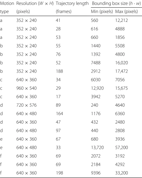
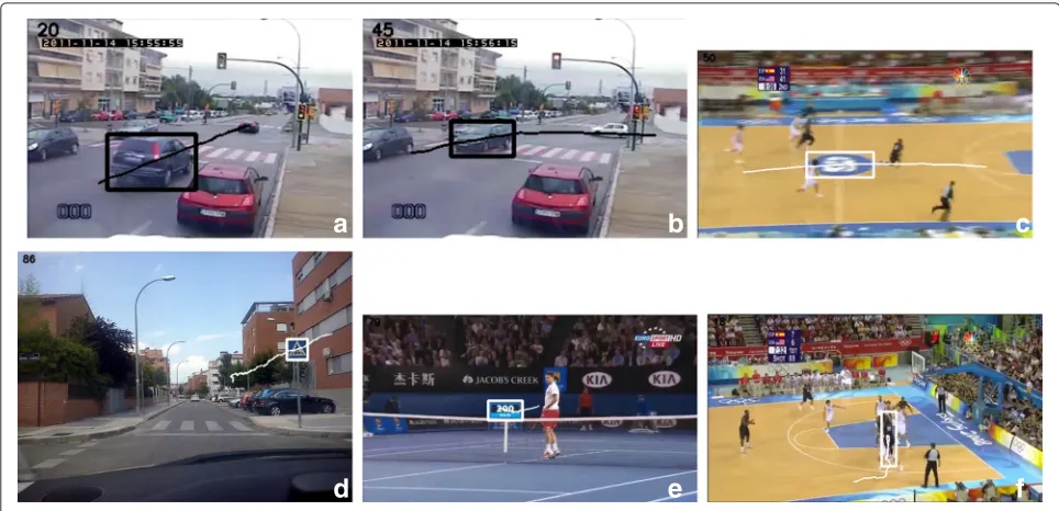
To test the performance of the interpolation algorithms, 19 short (a few seconds long) video clips were selected and manually annotated. The clips were extracted from surveillance and broadcasted video and personal cam-eras. All the videos, annotations, source code, and a Python application can be downloaded from the project web page [20]. The objects were carefully annotated in every frame (which can involve more than one hun-dred frames each). Table 1 summarizes the main prop-erties of the videos selected for the test. The selection includes different object and/or camera motion types (see column motion type in this table), to check the algo-rithms against a number of situations. These include the following:
(a) Rigid object moving in straight path, static camera (b) Rigid object moving in curved path, static camera (c) Static object, with camera panning
(d) Static object, with camera translation (e) Static object, with camera zoom
(f) Non-rigid objects
Also, Fig. 15 shows some sample images of the video data set.
a
b
Fig. 14Comparison of trajectories using cubic spline interpolationawithout andbwithtrajectory breaks. Normal key frames are marked withblack circles, while breaks are marked withwhite circles
ei=bpi ∪bgi−bpi ∩bgi (31)
where the first term denotes the union of the interpolated bounding box with the annotated one (or ground truth) and the second their intersection. For a given trajectory, the interpolation error is computed as the average of all partial overlap errors:
en= 1 M
M
ei (32)
Table 1Video data set summary
Motion Resolution (W×H) Trajectory length Bounding box size (h·w)
type (pixels) (frames) Min (pixels) Max (pixels)
a 352×240 41 560 12,212
a 352×240 28 616 4888
a 352×240 53 660 1856
b 352×240 55 1440 5508
b 352×240 76 1392 4800
b 352×240 52 7488 16,020
b 352×240 188 2912 17,472
c 640×360 34 6030 7056
c 960×540 29 12,920 15,675
c 640×360 17 3942 5270
d 720×576 89 240 4640
d 640×480 164 1176 6360
d 640×360 47 432 2480
d 640×480 97 440 2808
e 640×360 67 680 3936
e 640×480 33 13,720 57,200
f 640×360 69 2072 3192
f 640×360 69 2184 4292
f 640×360 198 9396 33,200
See text for the description of the column motion type
where the subscript n indicates the interval between a pair of key frames. In this case, since we removed one half of the samples of the trajectory,n = 1 sample. Note that since we have to remove one half of the samples, we can create one test trajectory by removing the odd sam-ples and a second one removing the even samsam-ples. So, the computation ofe1is finally obtained as the mean value of e01ande11, where the superscript 0 means the error when the test trajectory is obtained by keeping the even sam-ples (that is, we start keeping the sample in 0, remove the sample in 1, keep the sample in 2, and so on), and sim-ilarly for the superscript 1. Likewise, e2is computed by constructing a new test trajectory removingn = 2 out of three samples. In this case, we can havee02,e12, ande22, and so the errore2is computed as the mean of these three values. We performed this computation until the interval n=20.
a
b
c
d
e
f
Fig. 15 a–fSample images of the video data set used in the experiments. See text for description
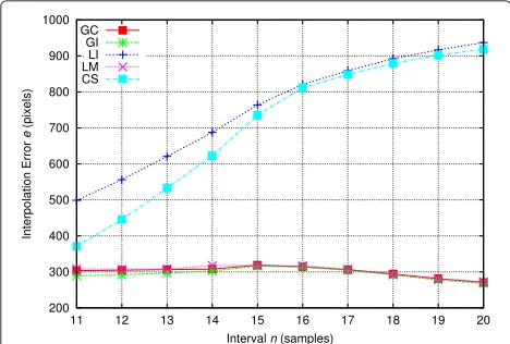
based on depth recovery but on interpolation from image coordinates, (LI) and (CS), yield the worst results. Table 2 shows the numerical results for the overall performance of the interpolators for different values of the intervaln.
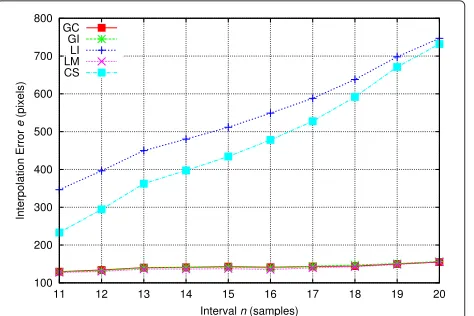
In order to make a more detailed analysis of the per-formance of the interpolators, we next present partial results considering the different types of object and cam-era motions. Figure 17 shows the mean error using only the trajectories of rigid objects moving in a straight path with great depth variations. In this case, the algo-rithms using depth recovery performed similarly and better than those using interpolation from the image coordinates.
Fig. 16Overall interpolation error
However, when the object follows a curved path, algorithms using cubic splines can model the object motion better. As can be seen in Fig. 18, the inclu-sion of a cubic spline interpolation improves the per-formance. In this case, the algorithm proposed in this paper (GC) yields the best results, since the objects also exhibits depth variations. The algorithms which com-pute straight paths between key frames decrease their performance.
When considering static objects but non-static cameras, the results are quite similar. If we analyze the trajectory on the image plane of a static object recorded with an on-board camera, we get the results shown in Fig. 19. In this case, the situation is equivalent to an object in front of a static camera moving in the opposite direc-tion, so that the same comments made before are valid here, that is, the algorithms using depth recovery perform better than those interpolating from image coordinates. However, since the videos are recorded with on-board cameras, camera vibration adds a random shift to the object trajectories, which degrades the performance of all the interpolators.
Table 2Overall interpolation erroren(pixels)
Intervaln(samples) GC GI LI LM CS
5 332.9 356.0 362.5 360.3 331.3
10 610.2 612.5 649.7 623.8 588.2
15 815.5 832.0 937.9 840.8 889.4
Fig. 17Results for straight paths with depth variations, static camera
Next, we obtained results for a static object while the camera is panning. In this case, since neither the object depth nor the size changes significantly, the algo-rithms based on image plane interpolation perform bet-ter than those based on depth recovery, as can be seen in Fig. 20. The main reason that makes the algorithms based on depth recovery decrease their performance is the nature of the annotations. In this case, although the object size in the image plane does not change, the annotations do, because they were done manually. This random change degrades the performance of those algorithms.
Next, we analyze the performance when the camera is zooming. In this case, the variation in the image plane of the object size due to the change in the camera’s focal length is not equivalent to the change in depth. In fact, an alternative study to the one developed in this paper can be done to model this type of trajectory. Nevertheless, Fig. 21 shows that it can be modeled accurately with the algorithms which use depth recovery (GC, GI, and LM).
Fig. 18Results for curved paths, static camera
Fig. 19Results for static object, with camera translation
The algorithm proposed in this paper is mainly intended to work with rigid objects. On the other hand, when working with non-rigid objects, like humans, geomet-ric assumptions do not hold, and the results get worse. This is due to the fact that a change in object size is erroneously interpreted as a change in object depth, and non-rigid objects can change their size in the image with-out changing their depth in space. For instance, the image of a man while crouching can reduce its bounding box height while maintaining the same distance from the cam-era. In order to analyze the performance for non-rigid object annotation, Fig. 22 shows the results for this kind of object. As can be seen, the results are a little worse than before, although all interpolators analyzed perform simi-larly, with a small advantage for the algorithms based on cubic splines.
5 Conclusions
In this paper, we have presented an alternative method that interpolates the bounding box annotations between
Fig. 21Results for static object, with camera zoom
key frames for video labeling. The method is based on a 3D reconstruction of the bounding box using the provided annotations, based on the geometric properties of the ele-ments involved. Once the 3D coordinates are computed, the interpolation of the bounding box for the remaining frames is performed in spatial coordinates, using cubic spline interpolation, and finally projected onto the image plane. The algorithm has been evaluated using a selected set of video clips that includes different types of object and camera motions and compared with other interpo-lation algorithms proposed in the literature. The results show a good performance, especially when considering rigid objects moving in trajectories with great variation in depth, where the accuracy of the interpolated bounding boxes is higher than the other evaluated algorithms. Since bounding box interpolation is a specific part of any anno-tation tool, we believe that the proposed algorithm can be a good alternative for all these tools when accurate object annotations are required.
Fig. 22Results for non-rigid objects
Competing interests
The authors declare that they have no competing interests.
Acknowledgements
This research was supported by projects CCG2014/EXP-055 and TEC2013-45183-R.
Received: 26 May 2015 Accepted: 7 February 2016
References
1. M Everingham, LV Gool, C Williams, J Winn, A Zisserman, The PASCAL visual object classes (VOC) challenge. Int. J. Comput. Vis.88, 303–338 (2010)
2. J Deng, W Dong, R Socher, LJ Li, K Li, L Fei-Fei, inIEEE Conf. Computer Vision and Pattern Recognition. ImageNet: a large-scale hierarchical image database (IEEE, New York, 2009)
3. B Russell, A Torralba, K Murphy, W Freeman, LabelMe: a datadata and web-based tool for image annotation. Int. J. Comput. Vis.77(1), 157–173 (2008)
4. L von Ahn, L Dabbish, inProceedings of the Conference on Human Factors in Computing Systems. Labeling IImage with a computer game (ACM, New York, 2004)
5. A Sorokin, D Forsyth, inIEEE Conference on Computer Vision and Pattern Recognition Workshops. Utility data annotation with Amazon Mechanical Turk (EEE, 2008), pp. 1–8
6. M Kipp, inProceedings of the 7th European Conference on Speech Communication and Technology. Anvil - A generic annotation tool for multimodal dialogue (INTERSPEECH, Aalborg, 2001), pp. 1367–1370 7. C Vondrick, DCR Patterson, Efficient scaling up crowdsourced video
annotation. Int. J. Comput. Vis.101(1), 184–204 (2012)
8. V Badrinarayanan, F Galasso, R Cipolla, inIEEE Conf. on Computer Vision and Pattern Recognition. Label propagation in video sequences (IEEE, New York, 2010)
9. C Liu, WT Freeman, EH Adelson, Y Weiss, inIEEE Conference on Computer Vision and Pattern Recognition. Human-assisted motion annotation (IEEE, New York, 2008)
10. A Agarwala, A Hertzmann, DH Salesin, SM Seitz, inACM Transactions on Graphics. Keyframe-based tracking of rotoscoping and animation (ACM, New York, 2004)
11. Z Kalal, K Mikolajczyk, J Matas, Tracking-learning-detection. Pattern Anal. Mach. Intell.34(7), 1409–1422 (2012)
12. D Doermann, D Mihalcik, inInt. Conf. on Pattern Recognition. vol. 4. Tools and techniques for video performance evaluation (IEEE, New York, 2000) 13. MA Serrano, J García, MA Patricio, JM Molina, inDistributed Computing and
Artificial Intelligence. vol. 79. Interactive video annotation tool (Springer-Verlag, Berlin - Heidelberg, 2010), pp. 325–332 14. J Yuen, B Russell, C Liu, A Torralba, inIEEE Int. Conf. Computer Vision.
LabelMe video: building a video database with human annotations (IEEE, New York, 2009)
15. JH Lee, KS Lee, GS Jo, inProceedings of the International Conference on Information Science and Applications (ICISA). Representation method of the moving object trajectories by interpolation with dynamic sampling (IEEE, New York, 2013), pp. 1–4
16. KS Lee, AN Rosli, IA Supandi, GS Jo, Dynamic sampling-based interpolation algorithm for representation of clickable moving object in collaborative video annotation. Neurocomputing.146, 291–300 (2014) 17. M Unser, Splines: a perfect fit for signal and image processing. Signal
Process. Mag.16(6), 22–38 (1999)
18. R Hartley, A Zisermann,Multiple View Geometry in Computer Vision, 2nd ed. (Cambridge University Press, Cambridge, 2003)
19. E Jones, T Oliphant, P Peterson, et al., SciPy: Open source scientific tools for Python (2001). http://www.scipy.org/. Accessed 15 Feb 2016 20. P Gil-Jiménez, TrATVid annotation tool. http://agamenon.tsc.uah.es/