Alternative method: outlier treatments with Box Jenkins and neural network via interpolation method

*Corresponding author: [email protected]

2018 UTHM Publisher. All right reserved. e-ISSN: 2600-7924/penerbit.uthm.edu.my/ojs/index.php/jst

Alternative Method: Outlier Treatments with Box-Jenkins and Neural

Network via Interpolation Method

Norsoraya Azurin Wahir*, Maria Elena Nor, Mohd Saifullah Rusiman and G. P. Khuneswari

Department of Mathematics and Statistics, Faculty of Applied Sciences and Technology, University Tun Hussein Onn Malaysia.

Received 30 September 2017; accepted 17 May 2018; available online 1 August 2018

1. Introduction

The presence of outliers in statistical data is an important issue especially when involving forecasting. The observation is called as an outlier when one of the data appears greatly different from the rest of the observations in the data [1]. Several factors that cause this outlier which are errors in data transmission, natural abnormal spikes in the data, periodic malfunction of measurement devices and others. The presence of this aberrant data gave bad influence on statistical method under assumption of normality and estimation. If this issue happens in the data, it does not represent the real value of the population and the estimation could also be greatly be affected. Detecting the outlier is the normal case and the modern software can be used to detect it in the data but, dealing or treat it is a difficult process and it is the main aspect to be concerned. The skewness coefficient, the data set and estimation method including results from the estimation also can affect and this had been proven [2]. Commonly, many researchers and statistician face this problem in handling outlier [3]. In order to reduce the error and deal with the present of outlier, there are several different opinions either to remove them, replace with the new value using special method or manual intervention. Some of researchers may remove it directly from the

data to achieve the best estimation [4]. Unfortunately, removing the outlier without replacing it with any new data may give invalid and undesirable result [5]. During the estimation of model parameter, the data that contains of outliers tend to loss the forecast accuracy and affecting the estimation [6]. In the real time traffic flow detection was shown that, the ability of some system can be enhance in adapting the changes of traffic patterns by treating the outlier before the forecasting was

applied. The detected outliers were

recommended and should be necessary to be treated in performing the short term traffic condition forecasting since it might indicate the changes in measurement errors, pattern changes and parameters [7]. Some researchers prefer to apply robust method as outlier treatment. The robust method was applied to estimate the model parameters with the presence of outlier and all the outliers were treated in same techniques [8]. Due to this reason, some robust method performs well and performs poor [9]. This is because the robust method cannot find the information about the individual outlier and may cause inaccurate forecast. The locations and types of outlier must be identified first before the treatment is applied. Then, the detected outlier must be treated with suitable method. Some researchers also considered outlier as missing data and assumed as time series model for the

Abstract: Outliers represent the points that greatly diverge and act differently from the rest of the points. These kinds of phenomenon usually happen in the data especially in time series data. The presence of this outlier gave bad effect in all statistical method including forecasting if there are no actions on it. Thus, this paper discusses alternative methods which are linear interpolation and cubic spline interpolation to the time series data as outlier treatment. Assuming outlier as missing value in the data, the outlier were detected and the results were compared using forecast accuracies by two popular forecasting model, Box-Jenkins and neural network. The monthly time series data of Malaysia tourist arrival were used in this paper from 1998 until 2015. The result indicates that the improved time series data using the linear interpolation and cubic spline interpolation showed great performance in forecasting than the original data series.

123

contaminated series and to replace the new value with interpolation method from the

missing data, [10,11]. Additionally, to

interpolate the outlier, missing elements, and to detect fraud, interpolation method was used by applying two algorithms on actual data. Obtained results from the simulation showed the better performance for NMF algorithms comparing with the ALS algorithm. For the

simulation, long-term (hourly) actual

electricity consumption data was used after applying the interpolation method [12]. For measuring HRV in daily lives, cubic-spline and linear interpolation were employed in completing the missing RRIs to reduce the noise and artefact. Evaluation of RRI measurement status, exclusion of RRI outlier, and complement of missing RRIs show that the technique is applicable for managing long term time-series and can enhance the correctness of HRV frequency domain particularly in several estimation algorithms while using as a RRI outlier processing tool for ECGs than the commonly used methods [13].Thus, this paper follows the method which was employed in the business Tankan surveys [14]. In this study the outlier is considered as missing value and handled by using various techniques such as linear and

cubic-spline interpolation methods by

replacing the missing values with the new improved series values. Then, the outliers were identified by using fit ARIMA distribution method through the SAS software. This paper also presents the comparison between Box-Jenkins and neural-network approaches by

using both linear and cubic-spline

interpolation methods in terms of forecast accuracy. All the enhanced series were compared with the original values from both approaches. Finally, discussion of each outlier in the data series and the comparisons conducted before and after the outlier treatment are presented.

2. Materials and Method

In this study, monthly time series data of tourist arrivals in Malaysia from 1998 to 2015 were used which were recovered from the website of Ministry of Malaysia Tourism. After applying both of the interpolation methods, the new set of data was called improved time series data. All the missing values were regarded as outlier in this data

series [12]. After that, all the outliers were identified through the ARIMA fit distribution. The interpolation method was used to estimate

new values of the function y(x) for any values

between x_0, and x_n with the values of y_0, to y_n [15]. In other words, this method also was used to generate new values for the missing data at (x,y) locations in the data depending on the closest points.This study mainly focuses on outlier treatment rather than detection of all the outlier which were replaced by using linear and cubic-spline interpolation methods. To indicate any changes before and after the outlier treatment, the original Box-Jenkins time series data and neural-network models were evaluated and analyzed with the new improved series from the same approach for using forecast accuracy. Several statistical softwares were used in this study like SAS, Minitab, SRS1Spline, and S-PLUS to analyze the data.

Linear Interpolation

The simplest form of interpolation if the linear interpolation method that joints two consecutive data points with a direct line. The outlier can be estimated directly by using the equation of linear interpolation as shown in equation (1).

𝑓 (𝑥) = 𝑏0+ 𝑏1(𝑥 − 𝑥0) (1)

Where,

𝑥 = The nondependent variable (time of

the missing observation)

𝑥0= A known value of the nondependent

Variable (time point of the missing observation)

𝑓1(𝑥) = The value of the dependent variable

for a value 𝑥 of the nondependent variable (the

missing observation)

From Equation (1),

𝑏0= 𝑓(𝑥0) (2) and

𝑏1 =

𝑓(𝑥1) − 𝑓(𝑥0)

𝑥1− 𝑥0

(3)

where,

𝑓(𝑥0) and 𝑥0 = starting points of the gap

124 Cubic-Spline Interpolation

One of the common interpolation

techniques is Cubic-spline interpolation

method as it can produce more smooth and seamless curves. The general equation of cubic-spline interpolation is presented in Equation (4).

𝑆𝑖(𝑥) = 𝑎𝑖(𝑥 − 𝑥𝑖)3+ 𝑏𝑖(𝑥 − 𝑥𝑖)2+

𝑐𝑖(𝑥 − 𝑥𝑖) + 𝑑𝑖

for 𝑥 ∈ [𝑥𝑖 , 𝑥𝑖+1] (4)

Where,

𝑎𝑖, 𝑏𝑖, 𝑐𝑖 and 𝑑𝑖 are constant values

The third order polynomial should satisfy the following conditions:

i. The 𝑆𝑖(𝑥) has to interpolate the 𝑦

values at the piece knots of 𝑥𝑖 and

𝑥𝑖+1, 𝑌𝑖 = 𝑆𝑖(𝑥𝑖), 𝑌𝑖+1= 𝑆𝑖(𝑥𝑖+1),

ii. Cubic polynomials 𝑆𝑖(𝑥) and 𝑆𝑖+1(𝑥)

over adjoining pieces with a common interior knot at 𝑥𝑖 which must have same value at the common knot.

iii. Cubic 𝑆𝑖(𝑥) and 𝑆𝑖+1(𝑥) over

adjoining pieces with common knot must have same first derivative value at the common identity as 𝑆_𝑖′(𝑥𝑖) =

𝑆𝑖′(𝑥𝑖+1)

iv. Cubic 𝑆𝑖(𝑥) and 𝑆𝑖+1(𝑥) over

adjoining pieces with common knot must have same second derivative

value at the common identity

as 𝑆𝑖′′(𝑥𝑖) = 𝑆𝑖′′(𝑥𝑖+1)

v. Second derivative at the end points of

entire data are zero where 𝑆𝑖′′(𝑥0) =

0 and 𝑆𝑁′′(𝑥𝑁) = 0

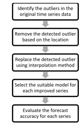
Thus, Fig. 1 indicates several steps for the outlier treatments that has been applied in this study.

Fig. 1 The process of outlier treatment by using the interpolation method

3. Results and Discussions

The Box-Jenkins and neural-network approach were tested in this research to interpolate the outliers by using interpolation methods. In this paper, the linear interpolation was used to generate the new data point which is a straight line and this may produce better fit of a smooth graph with less percentage of outlier in the data. Other than that, the cubic-spline interpolation also has same function as linear interpolation but, this interpolation will make the piecewise continuous curve while passing through the points of the graph.

Thus, Table 1 indicates the forecast accuracies between the original Box-Jenkins series that were treated before the outlier, and the improved time series data which is identified as the new series after applying the outlier treatment. Hence, all the data series were calculated and compared by using forecast accuracies which are Mean Square Error (MSE), Mean Absolute Deviation (MAD), and Mean Absolute Percentage Error (MAPE). The differences between MSE results from the original Box-Jenkins series and the improved series for both interpolation methods show massive improvement which was approximately more than 80,000 for linear interpolation and more than 85,000 for cubic spline interpolation from the original series. Moreover, similar findings were observed for the MAD and MAPE though, there are differences before and after the outlier

Identify the outliers in the original time series data

Remove the detected outlier based on the location

Replace the detected outlier using interpolation method

Select the suitable model for each improved series

125

treatment was applied in this series. From this result, cubic-spline showed the better results in interpolating the new data points after the linear interpolation.

Table 1 Forecast Accuracies of Original Box-Jenkins series comparing with Improved Time Series Data

Measurement

Before Outlier Treatment

After Outlier Treatment

Original Box-Jenkins

Improved Time Series Data

Linear Interpolation

Cubic-Spline Interpolation

MSE 259,693 178,389 173,415

MAD 175 172 163

MAPE 8.45% 8.06% 7.63%

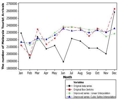
Fig. 2 presents time series plot of actual time series data, results of original

Box-Jenkins approach, improved linear

interpolation, and improved cubic-spline interpolation in the year 2015. Original data plot shows that the tourists are in extreme fluctuating trend for the whole year. At the end of the November 2015, the graph suddenly rises up to the highest limit which is nearly same as original series of Box-Jenkins graph. After applying the outlier treatment, the month of December 2015 indicates the normal observation like the previous months. The improved linear and cubic-spline interpolation graph show more stable pattern compared to the both of the original series of data. Thus, after the outlier treatment, two of the improved series plots show better performances rather than before the outlier treatments.

Fig. 2 Time Series Plots of Original Time Series Data, Original Box-Jenkins, Improved

Linear Interpolation, and Improved Cubic-Spline Interpolation

Table 2 presents the forecast accuracy between original neural-network approach and improved time series data for linear and cubic-spline interpolation which are applied before and after the outlier treatment. The MAD, MSE, and MAPE were compared and the results indicate that the MSE value for the

linear interpolation and cubic-spline

interpolation has huge improvement from the

original neural-network approach. The

difference of the linear interpolation from the original approach is more than 20,000. On the other hand, cubic-spline interpolation reached to 4446 from 32,516. These differences are presenting the massive variations after the application of outlier treatment.

Moreover, MAD and MAPE findings also indicate big differences comparing with the original neural-network approach. Values for MAD and MAPE for linear interpolation display about 50% gap from the values of original approach. At the same time, MAD and MAPE values for cubic-spline shows great improvements which are more than 50% comparing with the original MAD and MAPE values. Thus, all the values of forecast accuracy for both interpolation methods which are applied after the outlier treatment by using the neural-network strategy show great performances comparing with the original data series.

Table 2 Forecast Accuracies between Original Box-Jenkins series with Improved Time Series Data

Measurement

Before Outlier Treatment

After Outlier Treatment

Original Neural Network

Improved Time Series Data Linear

Interpolation

Cubic Spline Interpolation

MSE 32,516 12,323 4,446

MAD 174 73.82 60.17

MAPE 7.94% 3.47% 2.81%

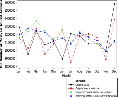
Fig. 3 demonstrates the time series plots of the original Malaysia tourist arrival data in the year 2015, the original Neural-Network approach, the improved series for linear interpolation, and cubic-spline interpolation data series of tourists arrival. The original data plot shows that the number of tourists are in fluctuating trend for the whole year from January to the end of December 2015. The pattern of the graph presents almost similar

Dec Nov Oct Sep Aug Jul Jun May Apr Mar Feb Jan 2700000 2600000 2500000 2400000 2300000 2200000 2100000 2000000 1900000 1800000 Month T h e n u m b e r o f M a la y s ia T o u ri s t A rr iv a ls

126

trend of the data series plot obtained from original neural-network where both of the graph show abrupt changes moving to the highest limits at the month of December 2015. After applying the outlier treatment as linear and cubic-spline interpolation methods, most of the months are displaying a little fluctuating behavior without having any abrupt changes like the previous two plots. Especially in between the month of November and December 2015, graph show normal behavior like other months. Thus, the number of tourists exhibit more stationary pattern after applying the interpolation methods while the cubic-spline interpolation method shows smooth curves than the linear interpolation as well as original series.

Fig. 3 Time Series Plot of Original Time Series Data, Original Neural-Network approach, Improved Linear Interpolation

method, and Improved Cubic Spline Interpolation strategy

In general, the outcomes of the forecast accuracies present positive results with good impact after the application of outlier treatment by using linear and cubic-spline interpolation methods in both of the Box-Jenkins and neural-network approaches for predicting the outliers in the original time series data. Moreover, all the improved data series show great performances especially the cubic-spline interpolation method followed by the linear interpolation approach.

4. Conclusion

In a nutshell, presence of outliers in data series especially in time series data could lead

to the bias in estimating the model and may affect the estimation of the variance in forecasting seriously. Thus in this study, the outliers has been considered as missing value and handled by using linear and cubic-spline interpolation methods as outlier treatment. Original data series are used in this research for both of the Box-Jenkins and neural-network approaches to interpolate the outlier of the Malaysia tourist arrival data. Both approaches were examined and compared with the improved series to evaluate the differences before and after the application of the outlier treatments. Linear interpolation method and cubic-spline interpolation method also were compared to get the best interpolation method in generating the new data series. In conclusion, the results acquired from all the enhanced series of Box-Jenkins and neural-network methods have smaller values for MAD, MSE, and MAPE than all the original data series. As the cubic-spline interpolation shows best performances followed by linear interpolation method, the forecast accuracy offers better result after applying the outlier treatment rather than before applying the treatment.

Acknowledgments

Authors would like to express their gratitude to the Malaysian Tourism Development Cooperation (MTDC) for providing the information of tourist arrivals. Authors also would like to thank University Tun Hussein Onn Malaysia (UTHM) for all the technical supports.

References

[1] Battaglias,F.(2006). “On Outlier Detection

in Multivariate Time Series”. Unpublished Paper Presented, Seminar in the University of Liverpool, United Kingdom.

[2] Álvarez, E., García-Fernández, R. M.,

Blanco-Encomienda, F. J., & Muñoz, J. F. (2014). “The Effect of Outliers on the Economic and Social Survey on Income and Living Conditions” in World Academy of Engineering and Technology,

International Journal of Social,

Behavioral, Education, Economic,

Business and Industrial Engineering, Vol. 8. No. 10 pp. 3268-3272.

Dec Nov Oct Sep Aug Jul Jun May Apr Mar Feb Jan 2600000

2500000

2400000

2300000

2200000

2100000

2000000

1900000

1800000

Month

T

h

e

N

u

m

b

e

r

o

f

M

a

la

y

s

ia

T

o

u

ri

s

t

A

rr

iv

a

ls

Original series Original Neural Network Improved Series: Linear Interpolation Improved Series: Cubic Spline Interpolation

127

[3] Pigott, T. D., (2001). “A Review of

Methods For Missing Data” in

Educational Research and Evaluation, Vol. 7. No. 4 pp. 353-383.

[4] Judd, C. M., & McClelland, G. H.,

(1989). Data analysis: A model

comparison approach. Harcourt Brace Jovanovich. San Diego, CA.

[5] Orr, J., Sackett, R. & Dubois, C. (1991). “Outlier detection and treatment in I/O psychology: A survey of researcher beliefs and an empirical illustration” in

Personnel Psychology, Vol. 44. No 3 pp.

473-486.

[6] Chen, C., & Liu, L. M. (1993).

“Forecasting time series with outliers” in

Journal of Forecasting, Vol. 12. No. 1 pp. 13-35.

[7] Cemgil, T., Kurutmaz, B., Cezayirli, A.,

Bingol, E., & Sener, S. (2017).

Interpolation and fraud detection on data collected by automatic meter reading. In

Smart Grid and Cities Congress and Fair (ICSG), 2017 5th International Istanbul

pp. 51-55.

[8] Martin, R. D., (1981). Robust Estimation

for Time Series Auto-Regression in Robustness in Statistics. Applied Time Series Analysis II. New York Academic Press. New York.

[9] Alice, C. and Bovas, A., (1989).

“Comparison of Parameter Estimation Methods in Time Series Outliers: A

Simulation Study” in ASA Proceedings,

Business & Economic Statistics Section, Vol. 4. pp. 83-92.

[10]Shittu, O. I., (2008). “Accommodation of

Outliers In Time Series Data: A Case

Study” in Asian Journal of Mathematics

and Statistics, Vol 1. No. 1, pp. 24-33. [11]Xie, Z., (1993). Case Study IX In Time

Series Analysis : Miscellaneous Cases Study. World Scientific Publishing.Plc. London. UK

[12]Guo, J., Huang, W., & Williams, B. M. (2015). Real time traffic flow outlier

detection using short-term traffic

conditional variance prediction.

Transportation Research Part C: Emerging Technologies, No 50, pp. 160-172.

[13]Eguchi, K., Aoki, R., Shimauchi, S.,

Yoshida, K., & Yamada, T. (2018). Rr Interval Outlier Processing For Heart Rate Variability Analysis Using Wearable

ECG Devices. Advanced Biomedical

Engineering, Vol 7, pp. 28-38.

[14]Atsushi, I., Shunsuke. E. and Tetsuya.

S.,(2010). “Treatment of Outliers in Business Surveys: The Case of Short-Term Economic Surveys of Enterprises in

Japan (Tankan)” in Bank in Japan

Working Paper Series. Japan. Vol.10. No. E-8.

[15]Chin Foon Khoo, Sharifah Sakinah Syed

Ahmad, and Zuraini Othman. (2008).