http://www.sciencepublishinggroup.com/j/acm doi: 10.11648/j.acm.20190803.11
ISSN: 2328-5605 (Print); ISSN: 2328-5613 (Online)
A Fifth-fourth Continuous Block Implicit Hybrid Method for
the Solution of Third Order Initial Value Problems in
Ordinary Differential Equations
Adoghe Lawrence Osa
1, Omole Ezekiel Olaoluwa
21Department of Mathematics, Ambrose Alli University, Ekpoma, Edo State, Nigeria 2
Department of Mathematics, Federal University of Technology, Akure, Nigeria
Email address:
To cite this article:
Adoghe Lawrence Osa, Omole Ezekiel Olaoluwa. A Fifth-fourth Continuous Block Implicit Hybrid Method for the Solution of Third Order Initial Value Problems in Ordinary Differential Equations. Applied and Computational Mathematics. Vol. 8, No. 3, 2019, pp. 50-57. doi: 10.11648/j.acm.20190803.11
Received: January 30, 2019; Accepted: March 17, 2019; Published: August 12, 2019
Abstract:
In this paper, block method was developed using method of collocation and interpolation of power series as approximate solution to give a system of non linear equations which is solved to give a continuous hybrid linear multistep method. The continuous hybrid linear multistep method is solved for the independent solutions to give a continuous hybrid block method which is then evaluated at some selected grid points to give a discrete block method. The basic properties of the discrete block method were investigated and found to be zero stable, consistent and convergent. The derived scheme was tested on some numerical examples and was found to give better approximation than the existing method.Keywords:
Collocation, Interpolation, Approximate Solution, Continuous Block Method, Discrete Block Method, Convergence1. Introduction
This paper considered the approximate methods of solution of the general third order initial value problems of the form
(
) ( )
0( )
0( )
0''' , , ', '' , 0 , ' 0 , '' 0
y =f x y y y y =a y =b y =c (1)
Where f is continuous within the interval of integration. Equation (1) has a wide application in Engineering, Thermodynamics and other real life problems; hence it is important for researchers to study the methods of solving (1).
However, only a limited number of analytical methods are available for solving (1), hence the resort to numerical approximation methods. The well-known conventional method for solving (1) is to reduce it to a system of first order differential equations, Fatunla 1988)
The reduction of such problems of type (1) to systems of first-order equations, leads to serious computational burden as well as wastage in computer time
It has been reported that direct method for solving (1) is
more efficient than the method of reduction to system of first order ordinary differential equations [1-18].
Implicit linear multistep methods which have better stability properties than explicit methods have been developed for the solution of (1) above [3-6, 10, 13, 17], among others proposed multi-derivative linear multistep method were implemented in predictor-corrector mode. Although successes were recorded by these methods, the major setback of the predictor-corrector is that apart from the computational burden associated with the method, the predictors are in reducing order of accuracy; hence, the method does not give better approximation.
To cater for these set-backs of the predictor corrector methods, researchers developed block methods. Block method have been developed individually using different approximate solutions (see [1-2, 13, 15-17]). It was found out that block method is more efficient in terms of time of execution, cost effectiveness and accuracy than the predictor-corrector method.
new method preserves the traditional Runge-kutta advantage of being self-starting. The paper is organized as follows: Section two considers the method and the materials for the development of method. Section three considers the analysis of the basic properties of the method which include, zero stability, consistency and convergent. Section four considers numerical examples where the efficiency of the derived method is tested on some numerical examples. Section five considers the discussion of results and the finally chapter six is the conclusion.
2. Development of Method
Taylor series expansion of exponential function is adopted as a basis function for the approximation of (1)
1
0
( ) ( )
r s j j j
Y x a
φ
x+ −
=
=
∑
(2)Where ( ) !
j j
x x
j
φ = and
w s
j'
are the coefficients to bedetermined and a polynomial of degree
r
+ −
s
1
. The 5-Point hybrid Computational method is constructed by imposing the following conditions on (2).(3)
(4)
Putting (1) into (4) gives
( , , ', '') j( ) '''
f x y y y =φ x (5)
Here, a step-length of 5
4
k= with constant step size
1 4
h= . Interpolating (3) at , 1 1 3, , 4 2 4 n j
x=x+ j= and
collocating (4) at , 0 1 5 4 4
n j
x=x + j=
gives a system of
non-linear equation of the form
QX =B (6)
Solving (6) for the aj,j=0(1)8 and substituting back into (2) above and after much algebraic simplification yield a method of the form
3 1
( ) ( ) ( ) ( )
0 0
k k
y x x y h x f v x fn v
j n j j n j
j α j β β
−
= ∑ + + ∑ + + +
= = (7)
where
y x
( )
is the numerical solution of the ivp and 1 1 3 5, , , 4 2 4 4
v= . and are constants and fn j+ = f x( n j+ ,yn j+ ,y′n j+ ,yn j′′+ )
[
]
(0) ( ) 3
1 0
(
)
(
)
(
)
!
k i
i i
m i n i n i m
i
jh
A Y
e y
h
d f y
b F Y
i
− +
=
=
∑
+
+
(8)Where
( )
( )
( ) 1
1 1
3 ( )
1 4
1 1
2
2 2
1 ( )
2
1 1 ( ) 1
4 4
1 4
1
( ) 4
3 3
3
4 4
4 ( )
5 5
5
4 4
4
, , ,
i n
n n
i
n n
n n
i n
i
n n n
m m n n
n i
n n
n
n i
n n
n
y
y f f
y
y f
f
y f y
Y f Y y f y f
y f y
f
y f
y
+
+ +
− +
+ +
−
+ + +
+
−
+ + +
+ +
+
= = = =
1
n
y
−
Thus (6) reduces to the following
(0)
1 0 0 0 0 0 1 0 0 0 0 0 1 0 0 0 0 0 1 0 0 0 0 0 1 A
=
0 1 2 0
3129 1
1 0 0 0 0 0 0 0 0
0 0 0 0 32 2580480
4
317 1
0 0 0 0 1 1 0 0 0 0 0 0 0 0
0 0 0 0 8 40320
0 0 0 0 1 2
9
, , ,
0 0 0 0 1 3 0 0 0 0
0 0 0 0 32
4 0 0 0 0 1
1
0 0 0 0 1 0 0 0 0
0 0 0 0 1
2 5
25 0 0 0 0
0 0 0 0 4
32
e e e d
= = = = 783 0 0 0 0
40960 89 0 0 0 0
2520 29125 0 0 0 0
516096 − 0
975 1931 173 1539 139 516096 12910240 184320 286720 2580480
367 19 61 89 1
20160 2016 10080 40320 2880 16119 2187 423 1539 243 286720 143360 28672 286720 286720
73 1 11 5 1
630 90 315 504 630
101875 625 19375 625 516096 258048 258048 7
b − − − − − − = − − − 1375 3728 516096
1 2 1
when 1
1231 1 0 0 0 0
0 0 0 0 80640
4
71 0 0 0 0 1 1 0 0 0 0
0 0 0 0 2016
0 0 0 0 1 2
123
, ,
0 0 0 0 1 3 0 0 0 0
0 0 0 0 2240
4 0 0 0 0 1
47 0 0 0 0 1 0 0 0 0 0 0 0 0 1
630 5
1525 0 0 0 0
0 0 0 0 4
16128
i
e e d
= = = = , 1
863 761 341 94 107 32256 40320 80640 80640 161280
34 37 17 101 1 315 1008 630 10080 630 3501 9 87 9 9 17920 2240 1792 560 3584
89 11 38 1 1 315 315 315 63 315 11875 625 3125 625 275 32256 8064 16128 16128 32256
b − − − − − = −
when i=2
2 2 2
95 1427 133 241 173 35 0 0 0 0
1152 5760 960 2880 5760 640
7 43 7 7 1 1
0 0 0 0 1 0 0 0 0
90 120 180 180 60 360 0 0 0 0 1
51 219 57 57 21
, ,
0 0 0 0 1 0 0 0 0
640 640 320 320 64 0 0 0 0 1
7 0 0 0 0 0 0 0 0 1
90 95 0 0 0 0
1152
e d b
− − − − = = = 3 0 640 16 2 16 7
0 45 15 45 90 125 125 125 125 95 384 576 576 384 1152
3. Basic Properties of the Methods
3.1. Order and Error Constant of the Main Method
Let the linear Operator defined on the method be [ ( ); ],y x h where
( ) ( ) ' (3 ) 0
[ ( ); ]
[
(
)
(
)]
k
o i i
m n i m i m
i
jh
y x h
A Y
y
h
d f y
b F y
i
− =
Expanding the form
Y
mandF y
(
m)
in Taylor Series and comparing coefficients in powers of h, we obtained. [ ( ); ] 0 ( ) 1 '( ) ... ( ) 1 1 1( ) 2 2 2( ) ...
p p p p p p
p p p
y x h C y x C hy x C h y x C +h + y + x C +h + y + x
∆ = + + + + + (10)
Theorem 1: The linear operator and the associated block method are said to be of order p if
0 1 ... p p 1 0, p 2 0, p 2 0, p 3 0
C =C = C =C + = C + = C + = C + ≠ Cp+3 is called the error constant. It implies that the local truncation error
is given by
3 3 4
4
( )
(
)
p p p
n k p
T
+=
C
+h
+y
+x
+
O h
+ (11) Expanding the block in Taylor Series gives3
' 2 '' 3 '''
0 0
' 2 ''
0
1
1 1 3929 995 1 1931 1 173 3 1539 139 5 4
( ) ( ) ( ) (1) ( ) ! 4 32 2580480 ! 516096 4 1290240 2 184320 4 286720 2580480 4 1
1 1 317 2
! 2 8 40320
q
q q q q q q
n n n n n
q q
q
n n n n
q
h
h y y hy h y h y
q q
h
y y hy h y q ∞ ∞ + = = ∞ = − − − − − − + − + − − − −
∑
∑
∑
3 ''' 30
3
' 2 '' 3 '''
0 0
367 1 19 1 61 3 89 1 5 ( ) ( ) ( ) (1) ( ) ! 20160 4 2016 2 10080 4 40320 2880 4 3
3 9 783 16119 1 2187 1 423 3 4
( ) ( ) ( ) ! 4 32 40960 ! 286720 4 143360 2 28672 4
q
q q q q q
n q
q
q q q q
n n n n n
q q h h y q h h y y hy h y h y
q q ∞ + = ∞ ∞ + = = − − + − + − − − − − − + −
∑
∑
∑
( ) 3
' 2 '' 3 '''
0 0
' 2 ''
0
1539 243 5 (1) ( ) 286720 286720 4
1 1 89 73 1 1 1 11 3 5 1 5
( ) ( ) ( ) (1) ( ) ! 2 2520 ! 630 4 90 2 315 4 504 630 4 5
5 25 29125 4
! 4 32 516
q q
q
q q q q q q
n n n n n
q q
q
n n n n
q
h h
y y hy h y h y
q q
h
y y hy h y q ∞ ∞ + = = ∞ = + − − − − − − + − + − − − −
∑
∑
∑
3 ''' 30 0 0 0 0 0
101875 1 625 1 19375 3 625 1375 5 ( ) ( ) ( ) (1) ( ) 096 ! 516096 4 258048 2 258048 4 73728 516096 4
q
q q q q q
n q h h y q ∞ + = = − − + − +
∑
(12)and comparing the coefficients of h, the order of the block is p=6 with error constant
3
-82459 -4091 -53487 -13 1700375
, , , ,
7997698867200 62482022400 380842803200 5857689600 959723864064
P
C + =
3.2. Consistency
It is important that a linear multistep method satisfied the necessary and sufficient conditions. A numerical method is said to be consistent if the following conditions are satisfied.
i. The order of the scheme must be greater than or equal to 1 i.e. p≥1.
ii. 0 0, k j j j α α = =
∑
's are the coefficients of the firstcharacteristic polynomial
iii.
ρ
( )
r
=
ρ
'
( )
r
=
0
where r=1 , root of thecharacteristics polynomial
iv.
ρ
(3)( )
r =3!σ
( )
r forr
=
1
, σ(r) is the second characteristic polynomial.The first condition is a sufficient condition for the associated block method to be consistent [8, 9, 11-13].
3.3. Zero Stability of the Method
The general form of block method is given as
(0 ) ( )i mu[ i i ]
m m i m m i
A Y =A Y − +h B Y +B Y − (13) Applying (9-16) gives
(0) ( )i
A A
λ
−
1 0 0 0 0 0 0 0 0 1 0 1 0 0 0 0 0 0 0 1 0 0 1 0 0 0 0 0 0 1 0 0 0 1 0 0 0 0 0 1 0 0 0 0 1 0 0 0 0 1
= −
5 4 0, 0, 0, 0, 01
λ −λ = λ=
the above conditions
3.4. Region of Absolute Stability of the Method
In (14), we express the stability in the form below [4, 13, 18].
1
( ) ( )
M z = +V zB M−zA−U (14) Together with the stability function
( , ) det( ( ))
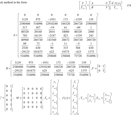
We express block method in the form 2
1 1
( )
i i
Y A U h f y
Y+ B V Y−
=
(16)
0 0 0 0 0 0
3129 975 1931 173 1539 139 2580480 516096 12910240 184320 286720 2580480
317 367 19 61 89 1 40320 20160 2016 10080 40320 2880
783 16119 2187 423 1539 243 40960 286720 143360 28672 286720 286720
89 73 1 11 5 1
2520 630 90 315 504 63
A
− −
− −
= − −
− −
0 29125 101875 625 19375 625 1375 516096 516096 258048 258048 73728 516096
− −
3129 975 1931 173 1539 139
0 1 2580480 516096 12910240 184320 286720 2580480 ,
29125 101875 625 625 625 1375 0 1 516096 516096 258048 258048 73728 516096
B V
− −
= =
− −
0 1 0 1 0 1 , 0 1 0 1 0 1 U
=
1 0 0 0 0 0 1 0 0 0 0 0 1 0 0 0 0 0 1 0 0 0 0 0 1 M
=
,
1 1
4 4
1 1
1
2 2 1
1 1
5
3 3
4
4 4
1 1
5 5
4 4
, ( ) , ,
n n
n n
n n n
n
m i i
n n
n n
n n
n n
y f
y f
y f y
y
Y f y Y Y y
y f y
y f
y f
+ +
+ + + +
− +
+
+ +
+ +
+ +
= = = =
Figure 1. Region of Absolute Stability of the Method.
4. Numerical Experiment
In this section, the efficiency and the performance the new developed methods is tested on five test problems. We present some numerical experiments widely solved [2, 14,
20]. The performance of the new developed method is examined on seven third-order initial value problems of ordinary differential equations. Tables 1-7 shows the comparison of our method with the selected problems in the existing methods [2, 14, 20] in terms of absolute errors.
Problem 1
''' '' ' 0, (0) 1, '(0) 0, ''(0) 1, 0 1
y −y + − =y y y = y = y = − ≤ ≤x
Exact soln:
y x
( )
=
cos
x
Problem 2''' 5 '' 7 ' 3 0, (0) 1, '(0) 0, ''(0) 1
y + y + y+ y= y = y = y = − ,
1, 0 x 1
− ≤ ≤
Exact soln:
y x
( )
=
e
−x+
xe
−xProblem 3
''' 3sin , (0) 1, '(0) 0, ''(0) 2, 0 1
y = x y = y = y = − ≤ ≤x
''' '(2 '' ') 1
(0) 1, '(0) , ''(0) 0, 0.01 2
y y xy y
y y y h
= +
= = = =
Exact solution: ( ) 1 1 2 2 2
x
y x inl
x +
= + −
Problem 5
''' 4
(0) 0, '(0) 0, ''(0) 1, 0.01
y x y
y = −= y = y = h=
Exact solution:
2
3 3
( ) cos(2 )
16 16 8
x
y x = − x + +
Problem 6
The non-linear boundary layer flow problem
( )
( )
( )
2 '''y +yy''=0, y 0 =0, ' 0y =0, '' 0y =1, h=0.1
This is the famous Blasius equation Problem 7
''' ', (0) 0, '(0) 1, ''(0) 2, 0.1
y = −y y = y = y = − h=
Table 1. Results of problem 1, h=0.01.
X Exact solution Computed solution Error in Proposed Method Error in [14]
0.0100000 0.999950000417 0.999950000417 0.0000e+00 6.72000e-07 0.0200000 0.999800006667 0.999800006667 1.1102e-16 1.34410e-06 0.0300000 0.999550033749 0.999550033749 4.4409e-16 2.01700e-06 0.0400000 0.999200106661 0.999200106661 5.8842e-15 2.68840e-06 0.0500000 0.998750260395 0.998750260395 2.6201e-14 3.35940e-06 0.0600000 0.998200539935 0.998200539935 8.3822e-14
0.0700000 0.997551000253 0.997551000253 2.0750e-13 0.0800000 0.996801706303 0.996801706303 4.4142e-13 0.0900000 0.995952733012 0.995952733013 8.4743e-13 0.1000000 0.995004165278 0.995004165280 1.5086e-12
Table 2. Results of problem 2, h=0.1/32.
X Exact solution Computed solution Error in our Method
0.0101563 0.999948773170 0.999948773170 7.9936e-15 0.0109375 0.999940619910 0.999940619910 1.1546e-14 0.0117188 0.999931869541 0.999931869541 1.5543e-14 0.0125000 0.999922523000 0.999922523000 2.2093e-14 0.0132813 0.999912581224 0.999912581224 3.0309e-14 0.0140625 0.999902045148 0.999902045148 4.0079e-14 0.0148437 0.999890915707 0.999890915707 5.1625e-14 0.0156250 0.999879193834 0.999879193834 6.4615e-14 0.0164063 0.999866880460 0.999866880460 8.2045e-14 0.0171875 0.999853976517 0.999853976517 1.0258e-13
Table 3. Results of problem 3, h=0.1.
X Exact solution Computed solution Error in our Method Error in [2]
0.100000 0.990012495834 0.990012495834 2.2204e-16 2.5934e-12
0.200000 0.960199733524 0.960199733524 4.4409e-16 1.1857e-11 0.300000 0.911009467377 0.911009467377 1.3323e-015 2.6224e-11 0.400000 0.843182982009 0.843182982009 3.8858e-015 4.7034e-11 0.500000 0.757747685671 0.757747685671 9.2149e-015 7.2700e-11 0.600000 0.656006844729 0.656006844729 1.8985e-014 1.0437e-10 0.700000 0.539526561853 0.539526561853 3.4084e-014 1.4049e-10 0.800000 0.410120128041 0.410120128041 5.7343e-014 1.8197e-10 0.900000 0.269829904812 0.269829904812 9.0095e-014 2.2736e-10 1.000000 0.120906917604 0.120906917604 1.3678e-013 2.7729e-10
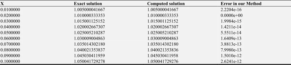
Table 4. Results of problem 4, h=0.01.
X Exact solution Computed solution Error in our Method
Table 5. Results of problem 5, h=0.01.
X Exact solution Computed solution Error in our Method
0.0100000 0.000049998750 0.000049998750 1.7896e-17 0.0200000 0.000199980001 0.000199980000 5.7085e-13 0.0300000 0.000449898762 0.000449898759 2.7015e-12 0.0400000 0.000799680068 0.000799680061 7.3797e-12 0.0500000 0.001249219010 0.001249218995 1.5592e-11 0.0600000 0.001798380777 0.001798380749 2.8358e-11 0.0700000 0.002447000710 0.002447000664 4.6545e-11 0.0800000 0.003194884367 0.003194884296 7.1128e-11 0.0900000 0.004041807602 0.004041807499 1.0308e-10 0.1000000 0.004987516655 0.004987516511 1.4336e-10
Table 6. Results of problem 5, h=0.1.
X Exact solution Computed solution Error in our Method (p=6) Error in [20] (p=7) Error [21] P=6
0.100000 0.004987516655 0.004987516655 2.1530e-013 1.1899e-11 2.0952e-09 0.200000 0.019801063624 0.019801063633 8.5054e-012 3.0422e-09 1.6375e-08 0.300000 0.043999572204 0.043999572273 6.8439e-011 7.7796e-08 1.1154e-07 0.400000 0.076867491997 0.076867492292 2.9415e-010 1.5559e-07 9.8800e-07 0.500000 0.117443317650 0.117443318550 8.9993e-010 3.0541e-07 3.0406e-06 0.600000 0.164557921036 0.164557923257 2.2216e-009 4.6102e-07 9.0126e-06 0.700000 0.216881160706 0.216881165434 4.7276e-009 3.1380e-07 1.6965e-05 0.800000 0.003194884367 0.003194884368 7.4418e-013 7.0374e-07 2.6772e-05 0.900000 0.004041807602 0.004041807603 1.1100e-012 1.0177e-06 3.8135e-05 1.000000 0.004987516655 0.004987516656 1.5931e-012 1.6528e-06 5.0596e-05
Table 7. Results of problem 6, h=0.1.
X Exact solution Computed solution Error in our Method Error in [3]
0.100000 0.00499995518745601 0.004999958334 3.147e-09 4.2730e-08 0.200000 0.0199986590802381 0.019998666843 7.760e-09 1.20759e-06 0.300000 0.0449898741025947 0.044989878832 4.730e-09 8.60719e-06 0.400000 0.0799573773516761 0.079957372944 4.410e-09 3.40900e-05 0.500000 0.124870047646537 0.124870034341 9.500e-09 9.74068e-05 0.600000 0.179677126361217 0.179677059379 1.3700e-08 2.25711e-04 0.700000 0.244303612900385 0.244303394383 1.2.00e-09 4.54547e-04 0.800000 0.318645979464674 0.318645494176 2.333e-08 8.08473e-04 0.900000 0.402568606213134 0.402567554422 1.110e-09 1.32622e-03 1.000000 0.495900337629337 0.495898354558 1.983e-06 2.02206e-03
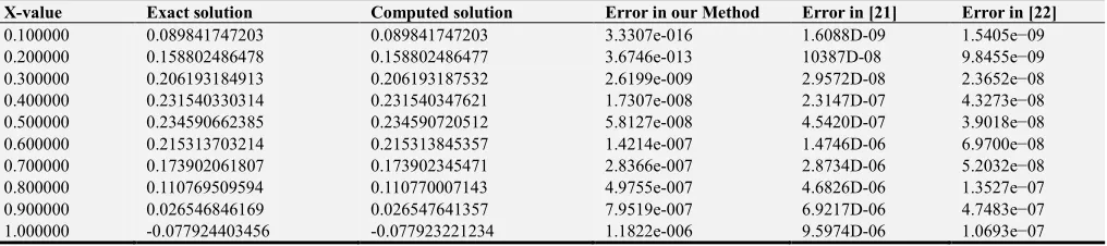
Table 8. Results of problem 7, h=0.1.
X-value Exact solution Computed solution Error in our Method Error in [21] Error in [22]
0.100000 0.089841747203 0.089841747203 3.3307e-016 1.6088D-09 1.5405e−09 0.200000 0.158802486478 0.158802486477 3.6746e-013 10387D-08 9.8455e−09 0.300000 0.206193184913 0.206193187532 2.6199e-009 2.9572D-08 2.3652e−08 0.400000 0.231540330314 0.231540347621 1.7307e-008 2.3147D-07 4.3273e−08 0.500000 0.234590662385 0.234590720512 5.8127e-008 4.5420D-07 3.9018e−08 0.600000 0.215313703214 0.215313845357 1.4214e-007 1.4746D-06 6.9700e−08 0.700000 0.173902061807 0.173902345471 2.8366e-007 2.8734D-06 5.2032e−08 0.800000 0.110769509594 0.110770007143 4.9755e-007 4.6826D-06 1.3527e−07 0.900000 0.026546846169 0.026547641357 7.9519e-007 6.9217D-06 4.7483e−07 1.000000 -0.077924403456 -0.077923221234 1.1822e-006 9.5974D-06 1.0693e−07
5. Conclusions
The development and implementation of a Fifth-fourth Continuous block implicit hybrid Method for the Numerical Solution of General Third Order Initial Value Problems in Ordinary Differential Equations is study in this research. In forming the method, the method of collocation approach was adopted by introducing off-grid points both at interpolation and collocations. The analysis of the method was studied and it was found to be consistent, convergent
References
[1] Fatunla, S. O. (1988): Numerical methods for initial value problems in ordinary differential equations, Academic press Inc. Harcourt Brace Jovanovich Publishers, New York. [2] A. Olaide Adesanya, D. Mfon Udoh and, A. M. Ajileye (2013):
A New Hybrid Block Method For The Solution Of General Third Order Initial Value Problems Of OrdinaryDifferential Equations: International Journal of Pure and Applied Mathematics Volume 86 No. 2, 365-375.
[3] Adoghe L. O, Ogunware B. G and Omole E. O (2016): A family of symmetric implicit higher order methods for the solution of third order initial value problems in ordinary differential equations: Journal of Theoretical Mathematics & Applications, 6 (3): 67-84.
[4] Adoghe L. O and Omole E. O (2018): Comprehensive Analysis of 3-Quarter-Step Collocation Method for Direct Integration of Second Order Ordinary Differential Equations Using Taylor Series Function. ABACUS (Mathematics Science Series) Vol. 44, N0 2, pp. 311-321.
[5] Awoyemi D. O (2001): A new Sixth –Order Algorithm for General Second Order Ordinary Differential Equations. International Journal of Computer mathematics, Vol 77, pp. 117-124.
[6] Awoyemi, D. O and Idowu, O. M. (2005): A class of hybrid collocation Method for third ordinary differential equations. International Journal of Computer Math, 82 (10), 1287-1293. [7] Atkinson K. E (1989): An introduction to Numerical Analysis,
2nd Edition, John Wiley and Sons, New York.
[8] Fatokun, J. O (2007): Continuous Approach for deriving Self –starting multistep methods for initial value problems in ordinary differential Equations. Journal of Engineering and Applied Sciences Vol. 2 (3) pp. 504-508.
[9] Jain. M. K, Iyengar, S. R. K, Jain, R. K (2008): Numerical Methods for scientific and engineering computations (fifth edition). New Age International Publishers Limited.
[10] Henrici, P. (1962): Discrete Variable method in ordinary differential equations, John Wiley and Sons, New York. [11] Kayode, S. J and A. Adeyeye (2011): A 3-step hybrid method
for direct solution of second order initial value problems, Aust. J. of Basic and Applied Sciences, 5, No. 12 (2011), 2121-2126.
[12] Lambert J. D (1973): Computational Methods in ODES. John Wiley & Sons, New York.
[13] Lambert J. D. (1991): Numerical methods for initial value problems in ordinary differential equation, New York, Academics Press Inc.
[14] Mohammed U. and R. B Adeniyi (2014): A Three Step Implicit Hybrid Linear Multistep Method for the Solution of Third Order Ordinary Differential Equations. Gen. Math. Notes, Vol. 25, No. 1, pp. 62-74.
[15] Samuel. N. Jator (2008): On the numerical integration of third order boundary value problems by a linear multistep method; International Journal of Pure and Applied Mathematics, Vol. 46, No 3,375-388.
[16] Skwame, Y., Sabo, J. & Kyagya, T. Y. (2017): The constructions of implicit one-step block hybrid methods with multiple off-grid points for the solution of stiff ODEs. JSRR, 16 (1): 1-7.
[17] Tumba, P., Sabo, J. & Hamadina, M., (2018): Uniformly Order Eight Implicit Second Derivative Method for Solving Second- Order Stiff Ordinary Differential Equations ODEs. Academic Journal of Applied Mathematical Sciences, 4: 43-48. [18] Ogunware B. G, Adoghe L. O, Awoyemi D. O, Olanegan O.
O., and Omole E. O (2018): Numerical Treatment of General Third Order Ordinary Differential Equations Using Taylor Series as Predictor. Physical Science International Journal, 17 (3): 1-8; DOI: 10.9734/PSIJ/2018/22219.
[19] Yakubu D. G., Manjah N. H, Buba. S. S, and Masksha. A. I. (2011): A family of uniform accurate Lobatto–Runge–Kutta collocation methods: Journal of Computational and Applied Mathematics., Vol. 30, N. 2, pp 315-330.
[20] Awoyemi D. O., Kayode S. J. and Adoghe L. O (2014).: A four–point fully implicit method for numerical integration of third-order ordinary differential equations, Int. J. Physical Sciences, 9 (1), 7-12.
[21] T. A. Anake, A. O. Adesanya. G. J. Oghonyon, and M. C. Agarana (2013): Block Algorithm For General Third Order Ordinary Differential, ICASTOR Journal of Mathematical Sciences Vol. 7, No. 2, 127 – 136.