A s s e s s m e n t
O
f
B o n e D e n s i t y a n d
S t r u c t u r e
I
n
T h e C a l c a n e u s
Charanjit Kang
University College London
Submitted for
The Degree o f Doctor of Philosophy The University of London
ProQuest Number: 10106939
All rights reserved
INFORMATION TO ALL USERS
The quality of this reproduction is dependent upon the quality of the copy submitted.
In the unlikely event that the author did not send a complete manuscript and there are missing pages, these will be noted. Also, if material had to be removed,
a note will indicate the deletion.
uest.
ProQuest 10106939
Published by ProQuest LLC(2016). Copyright of the Dissertation is held by the Author.
All rights reserved.
This work is protected against unauthorized copying under Title 17, United States Code. Microform Edition © ProQuest LLC.
ProQuest LLC
789 East Eisenhower Parkway P.O. Box 1346
Magnetic resonance imaging (MRI) has shown the potential to provide information
related to the microarchitecture of the trabecular bone matrix. Detailed measurements
of the structure of bone samples were made by histomorphometry and compared to
T2’ (%CV=6.3 ± 2.7 - 8.7 ± 5.0) measured with a specially implemented sequence,
PRIME (Partially Refocused Interleaved Multiple Echo), at 1.5 Tesla. After correction
for bone mass, T2’ in 12 samples was significantly correlated to trabecular perimeter
(r=-0.61,p=0.04), number density (r=-0.61,p=0.03) and width (r=-0.66,p=0.03),
demonstrating the ability of MRI to characterise these important measures of the
trabecular bone surface. This result strengthens the hypothesis that the sensitivity of
T2’ to osteoporosis-related bone changes is due to magnetic susceptibility effects in
which rapid transitions between bone and marrow create local magnetic field
inhomogeneities which result in a shortening of the T2’ relaxation time.
In-vivo measurements of bone mineral density (BMD) and ultrasound parameters
were made in the calcaneus of 55 postmenopausal women aged 43-87 years.
Calcaneal T2’ was measured in 32 women and was significantly correlated to BMD
(r=-0.79,p<0.0001) and ultrasound parameters (r=-0.59,p=0.0004). These 3 techniques
have not previously been compared in the same study population. Z scores for all
techniques were significantly different in normal and osteopenic women defined by
spine BMD. All BMD and ultrasound parameters were significantly different in
normal and osteopenic women after adjustment for age and years since menopause
(YSM), while T2’ was only significantly different before correction. T2’ was
significantly correlated to the number of vertebral fractures (r=0.38, p=0.03), as were
BMD and ultrasound. The only parameters that were significantly different (after
adjustment for age and YSM) between women with (n=19) or without (n=14)
vertebral fractures were the change in BMD of the calcaneus or lumbar spine over one
year. The calcaneus was shown to be a sensitive and precise site for the measurement
Errata
Page Line
17 10 Replace 1/T2'by 1/T2*
1 1 T 2 T 1*
17 31 R eplace--- by
T2* T2 { T 2 - T 2 * )
35 17 Replace ‘attenuating it or reflecting i f by ‘absorbing it or scattering it’
40 9,10 Replace A-by Y
40 17 Replace R2*= R2 + R2 by R2*= R2 + R2’
50 24 Replace ‘reflected and refracted’ by ‘absorbed and scattered’
65 15 R eplace‘hip’ b y ‘right hip’
73 6 Replace ‘one minute’ by ‘10 seconds’
124 7 In the sheep femur column of Table 3.5, replace the per./area value of
‘0.0883 ± 0.0015’ with the value ‘0.0088 ± 0.0015’
130 5 Insert at end of paragraph ‘Another explanation for the difference in
BMD between the two bone cube orientations is that with the
trabeculae parallel to the x-ray beam many photons vdll pass straight
through the gaps. Hence any non-linear effects between attenuation in
bone and attenuation in marrow substitute will be observed’
146 2 Replace ‘r=80’ by ‘r=0.80’
146 19 Replace ‘r=-0.77’ by ‘r=0.77’
146 20 Replace ‘r=-0.76’ by ‘r=0.76’ and replace ‘r=-0.80’ by ‘r=0.80’.
159 3 Replace ‘Table 4.13’ by ‘Table 4.12’
166 1 Replace whole line by ‘(r=0.74) compared to the anatomical ROI
(r=0.46) with a p-value of <0.01.’
166 3 Replace ‘does not have fixed transducers’ by ‘does not have tranducers
in a fixed position relative to a footplate.’
ABSTRACT... 2
CONTENTS... 3
FIGURES...10
TABLES...12
ACKNOWLEDGEMENTS... 14
GLOSSARY...15
CHAPTER ONE INTRODUCTION AND REVIEW... 19
1.1 OVERVIEW ... 19
1.2 OSTEOPOROSIS AND BONE L O S S ... 20
1.2.1 Mechanisms o f bone loss...20
1.2.2 The importance o f bone structure...21
1.2.3 The role o f bone mass measurement...21
1.2.4 Selection o f measurement site...22
1.2.5 The calcaneus...23
1.3 TECHNIQUES OF BONE MASS MEASUREMENT... 25
1.3.1 Dual and Single Energy Absorptiometry...25
1.3.1.1 Development... 25
1.3.1.2 Sources of error...25
1.3.1.3 Accuracy... 26
1.3.1.4 Morphometric X-ray absorptiometry (MXA)... 26
1.3.2 Quantitative Computed Tomography...27
1.3.2.1 Conventional... 27
1.3.2.2 Peripheral Quantitative Computed Tomography (pQCT)...27
1.3.3 Summary Table...28
1.3.4 Other Techniques...28
1.3.4.1 Compton scattering...28
1.3.4.2 Low angle x-ray scattering... 29
1.3.4.3 Radiogrammetry...29
1.3.4.4 Grading of trabecular patterns... 29
1.4 HISTOMORPHOMETRY... 32
1.4.1 Introduction...32
1.4.3 Parameters o f bone structure...34
1.4.4 Dynamic variables...34
1.4.5 Limitations...35
1.5 MAGNETIC RESONANCE IMAGING...35
1.5.1 Introduction...35
1.5.2 MR Theory...36
1.5.3 Magnetic susceptibility effects...39
1.5.4 Investigations o f magnetic susceptibility effects...41
1.5.5 Effect o f trabecular orientation to main magnetic fie ld...42
1.5.6 Measurement o f relaxation tim es...43
1.5.6.1 Asymmetric spin echo...43
1.5.6.2 Gradient echo... 43
1.5.6.3 Calculation of relaxation times... 44
1.5.7 Effect o f bone marrow...45
1.5.8 High Resolution MR imaging...46
1.5.8.1 Techniques... 46
1.5.8.2 In-vitro imaging... 47
1.5.8.3 In-vivo imaging... 48
1.5.9 ^'P Studies...49
1.6 ULTRASOUND... 50
1.6.1 Introduction...50
1.6.2 Theory...51
1.6.3 Relationship to bone structure and strength...53
1.6.4 In-vivo studies...55
1.6.5 Commercial instruments... 55
1.6.6 Instrument factors and measurement problems...57
1.6.6.1 Phase cancellation...57
1.6.6.2 Other factors... 58
1.6.7 Advances...58
1.7 MICROCOMPUTED TOMOGRAPHY...59
1.8 SUMMARY...59
C HAPTER TW O MEASUREMENT METHODS AND P R E C IS IO N ...61
2.1 INTRODUCTION... 61
2.2 SUBJECTS... 61
2.2.1 Description o f subject groups...62
2.2.2 Criteria fo r selection ofpostmenopausal group...64
2.2.2.1 Inclusion criteria... 64
2.2.2.2 Exclusion criteria...64
2.4.1.1 Spine and femur measurements... 65
2.4.1.2 Patient positioning for calcaneus scanning...66
2.4.1.3 Description of calcaneus scan modes... 67
2.4.1.4 Calcaneus scanning and analysis... 68
2.4.2 DXA in-vivo precision study...69
2.4.3 Morphometric X-ray absorptiometry...73
2.4.4 Density measurements o f bone samples with DXA...74
2.4.4.1 Vertebral bone cubes...74
2.4.4.2 Sheep femur samples...74
2.4.5 Density measurements o f bone samples by QCT....76
2.5 MAGNETIC RESONANCE IMAGING AT 1.5T...76
2.5.1 In-vivo measurements...76
2.5.2 In-vivo MRI precision study...82
2.5.3 MR measurements on bone samples...83
2.5.3.1 The FISPPSIF gradient echo sequence... 83
2.5.3.2 The HIRES spin-echo sequence... 84
2.5.3.3 Measurement of vertebral cubes... 85
2.5.3.4 Measurement of sheep femur samples... 86
2.5.4 In-vitro MRI precision study...91
2.5.5 Quality control...93
2.6 ULTRASOUND... 96
2.6.1 Measurements...96
2.6.2 Ultrasound in-vivo precision study...97
2.7 STATISTICAL ANALYSIS...99
2.7.1 Study design...99
2.7.2 Correlation analysis...99
2.7.3 Tests fo r differences between groups...100
2.8 SUMMARY... 101
CHAPTER THREE IN-VITRO INVESTIGATIONS... 102
3.1 INTRODUCTION... 102
3.2 M ETHODS... 103
3.2.1 Histology...103
3.2.1.1 Introduction...103
3.2.1.2 Resin embedding...103
3.2.1.3 Sectioning...104
3.2.1.4 Staining... 106
3.2.2.1 Introduction...108
5.2.2.2 Image analysis system... 108
3.2.2.B Measurement of histomorphometry parameters...109
3.2.2.4 Accuracy and Precision... 113
3.2.3 High resolution MR imaging...115
3.2.3.1 Introduction...115
3.2.3.2 Hardware...115
3.2.3.3 Image Acquisition... 116
3.2.4 M RI measurements at 1.5 T....118
3.2.5 Bone density measurements...122
3.3 RESULTS... 123
3.3.1 Histomorphometry...123
3 .3 .1.1 Precision of measurements... 123
3.3.1.2 Histomorphometry results... 123
3.3.1.3 Correlation within parameters...124
3.3.2 High resolution MR imaging...125
3.3.3 Bone Density Measurements...127
3.3.3.1 DXA of vertebral cubes... 127
3.3.3.2 DXA of sheep femurs... 128
3.3.3.3 Comparison of methods... 129
3.3.3.4 Structural effects with DXA scanning... 129
3.3.4 M RI measurements at 1.5 T....130
3.3.4.1 Measurement results... 130
3.3.4.2 Correlation of MRI measurements with bone density... 131
3.3.4.3 Correlation of MRI and histomorphometry results...132
3.3.4.4 Correction of MRI parameters using the HIRES sequence... 133
3.3.4.5 Correction of MRI parameters using measurement orientation... 134
3.4 SUMMARY POINTS... 135
3.5 DISCUSSION AND CONCLUSIONS... 136
3.5.1 Discussion...136
3.5.1.1 Correlations with density...136
3.5.1.2 Structure independent of density...136
3.5.1.3 T2’ versus T2*... 137
3.5.1.4 Relationship to osteoporosis...138
3.5.1.5 Confirmation of magnetic susceptibility effects...138
3.5.1.6 High Resolution MR imaging...138
3.5.2 Conclusions...139
CH A PTER FO U R IN-VIVO INVESTIGATIONS W ITH DXA AND ULTRASOUN D ...140
4.1 INTRODUCTION...140
4.2.1.2 Variation in bone density across the calcaneus... 144
4.2.1.3 Choice of optimum measurement sites... 144
4.2.1.4 Measurement results in the axial skeleton... 145
4.2.1.5 Correlations between bone sites...146
4.2.1.6 Summary Points...147
4.2.2 Ultrasound measurement results...147
4.2.2.1 Correlation within ultrasound parameters... 148
4.2.2.2 Ultrasound compared to DXA...149
4.2.2.S Summary Points... 152
4.2.3 Comparison between techniques...152
4.2.3.1 Correlations with age... 152
4.2.3.2 Patterns and rates of bone loss...156
4.2.3.3 Age dependence of ultrasound...159
4.2.3.4 Correlation between rates of change... 161
4.2.3.5 Effects of weight and height...161
4.2.3.6 Comparison of Z scores... 162
4.2.3.T Summary Points... 163
4.2.4 Discussion...162
4.2.4.1 Variation in bone density across the calcaneus...163
4.2.4.2 Calcaneus BMD compared to axial... 164
4.2.4.3 Correlation between ultrasound and axial BMD...164
4.2.4.4 Correlation between ultrasound and calcaneus BMD... 165
4.2.4.5 Fixed versus, anatomical ROIs...165
4.2.4.6 Patterns and rates of bone loss...166
4.2.4.7 Changes in ultrasound parameters with age... 168
4.2.4.8 Correlations between rates of change of the parameters... 169
4.2.4.9 Effect of weight and height on DXA and ultrasound parameters... 170
4.3 PREDICTION OF FRACTURE PREVALENCE... 170
4.3.1 Results...170
4.3.1.1 Details of subject groups... 170
4.3.1.2 Measurement results... 171
4.3.1.3 Correlation within fracture indices...171
4.3.1.4 Correlations between fracture and BMD parameters...171
4.3.1.5 Correlations between fracture and ultrasound parameters...172
4.3.1.6 Z scores...172
4.3.2 Summary Points...173
4.3.3 Discussion...174
4.3.3.1 Fracture and BMD... 174
4.3.3.2 Fracture and ultrasound... 175
4.4 CONCLUSIONS...176
CHAPTER FIVE IN-VIVO MRI AND COMPARISON OF TECHNIQUES... 178
5.1 INTRODUCTION...178
5.2 RESULTS IN NORMAL AND OSTEOPENIC WOMEN... 178
5.2.1 Subjects and Measurements...178
5.2.2 Relaxation times...181
5.2.3 Dependence on age and weight...182
5.2.4 Summary Points...184
5.3 COMPARISON TO DXA AND ULTRASOUND... 185
5.3.1 Correlations with DXA and ultrasound....185
5.3.2 Comparison o f Z scores by all measurement techniques...186
5.3.3 Comparison o f age related changes by all measurement techniques...187
5.3.4 Summary Points...188
5.4 PREDICTION OF VERTEBRAL FRACTURES... 188
5.4.1 Correlation with vertebral fracture...188
5.4.2 Fracture Z scores and comparison to DXA and ultrasound...189
5.4.3 Risk classification by different techniques...190
5.4.4 Summary Points...193
5.5 DISCUSSION AND CONCLUSIONS... 193
5.5.1 Discussion...193
5.5.1.1 Comparison of MRI results with the literature...193
5.5.1.2 Differences between study groups... 194
5.5.1.3 Age related changes in T2’ and T2*...195
5.5.1.4 Age related changes in T2...196
5.5.1.5 Effect of weight... 196
5.5.1.6 MRI and density... 197
5.5.1.7 Correlation with ultrasound...197
5.5.1.8 MRI and vertebral fracture...199
5.5.2 Conclusions...200
CHAPTER SIX CONCLUSIONS AND FUTURE WORK... 201
6.1 CONCLUSIONS... 201
6.2 SUGGESTIONS FOR FUTURE W O RK...203
6.2.1 Improvements in MRI measurements precision...203
6.2.2 Other measurement sites fo r MRI....203
6.2.3 Other M RI parameters...203
6.2.4 Matching the measurement orientation fo r MRI and Ultrasound...205
Figures
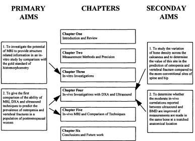
Figure 1.1 Aims o f the study and layout of thesis chapters... 20
Figure 1.2 Illustration o f the bones of the foot and magnetic resonance image of the heel...24
Figure 1.3 Changes in the trabecular patterns of the calcaneus with osteoporosis...31
Figure 1.4 T1 relaxation... 38
Figure 1.5 T2 and T2* relaxation... 39
Figure 1.6 Effect of the trabecular matrix on magnetic field homogeneity... 41
Figure 2.1 The foot positioning device used for DXA scanning of the calcaneus...66
Figure 2.2 The position of ROIs used in calcaneus scan analysis...69
Figure 2.3 ROIs used for the analysis of DXA scans of whole sheep femurs... 75
Figure 2.4 Measurement arrangement for subjects in the Siemens 1.5 T system ...78
Figure 2.5 Sequence diagram for PRIME... 78
Figure 2.6 PRIME image of heel to show placement of measurement R O I... 79
Figure 2.7 Signal Intensity variation with TE for PRIME images o f the calcaneus of a 80 year old fem ale... 79
Figure 2.8 PRIME image sequence for the calcaneus of a 80 year old female... 80
Figure 2.9 FISP: Steady state of the longitudinal and transverse magnetisation... 84
Figure 2.10 Measurement arrangement for MRI of bone cube samples... 86
Figure 2.11 Photographs of the measurement arrangement for MRI o f bone samples... 87
Figure 2.12 Measurement arrangement for MRI of sheep femurs...89
Figure 2.13 PRIME images o f a proximal sheep femur with marker and standard...90
Figure 2.14 MRI image o f a flood phantom showing the rapid loss of signal with distance from the coil...90
Figure 2.15 Illustration of the correction factor applied to MR images of sheep femur sam ples... 91
Figure 2.16 MRI QA measurements of the signal intensity o f the saline standard used with the bone cubes... 94
Figure 2.17 MRI QA measurements of the signal intensity o f the CuSO^ standard used with the sheep femur samples... 95
Figure 3.1 Preparation o f bone sections...105
Figure 3.2 Bone sections stained with toluidine blue... 107
Figure 3.3 The Magiscan image analysis system...109
Figure 3.4 Steps in the measurement o f histomorphometry parameters... I l l Figure 3.5 Photographs showing the image analysis step s... 112
Figure 3.6 Variation o f detected bone area in two bone cube samples with number o f fields measured...114
Figure 3.11 PRIME sequence images for a proximal and distal sheep femur sample...121
Figure 3.12 HIRES images of bone samples... 121
Figure 3.13 Illustration of different trabecular architecture at constant bone m ass... 125
Figure 3.14 High resolution images of a vertebral cube and a proximal sheep femur...126
Figure 4.1 Distribution of DXA BMD in the calcaneus... 144
Figure 4.2 Age dependence o f DXA parameters...157
Figure 4.3 Age dependence o f ultrasound parameters... 160
Figure 5.1 First six MRI PRIME images of the calcaneus of a 30 year old female... 180
Figure 5.2 Correlation between calcaneal T2’ and T2* in all subjects... 182
Figure 5.3 Age dependence of T2’ measured in the calcaneus... 183
Figure 5.4 Age dependence of T2 measured in the calcaneus... 183
Figure 5.5 Dependence of calcaneal T2* on years since m enopause... 184
Figure 5.6 Dependence of calcaneal T2 on years since menopause...184
Figure 5.7 BMD and BUA of the calcaneus in 55 postmenopausal women...191
Figure 5.8 Plots o f BMD, BUA and T2’ in the calcaneus o f 32 women with (circles) and without (diamonds) vertebral fractures... 192
Figure 5.9 MRI images of the calcaneus in three planes... 198
Figure 6.1 Sagittal and coronal images o f the patella...204
T ables
Table 1,1 Characteristics o f the major imaging techniques for quantifying bone mass... 28
Table 2.1 Number o f subjects measured by each technique... 63
Table 2.2 Description o f study groups...63
Table 2.3 Precision of DXA measurements of the calcaneus in 20 female volunteers measured three tim es... 71
Table 2.4 Summary of published studies on the precision o f DXA bone density measurements o f the calcaneus in-vivo...72
Table 2.5 Scan and analysis details for DXA measurement of bone samples... 75
Table 2.6 Precision of in-vivo MRI measurements of the calcaneus... 82
Table 2.7 MR sequence parameters for HIRES and FISPPSIF... 85
Table 2.8 Precision of MRI measurements in bone sam ples... 92
Table 2.9 Precision of in-vivo ultrasound measurements o f the calcaneus...97
Table 2.10 Summary of published studies on the precision o f ultrasound measurements of the calcaneus in-vivo...98
Table 3.1 Histomorphometry parameters...113
Table 3.2 Variation in directly measured histomorphometry parameters with number of fields sampled for 2 sheep femur samples...114
Table 3.3 Image parameters for high resolution M RI... 118
Table 3.4 Histomorphometry precision errors... 123
Table 3.5 Histomorphometry results for bone samples... 124
Table 3.6 Significant correlation coefficients within histomorphometry parameters for 12 vertebral cubes...125
Table 3.7 DXA measurements in 12 bone cube samples positioned with the trabeculae perpendicular and parallel to the x-ray beam... 128
Table 3.8 Summary of MRI measurement results for in-vitro sam ples... 131
Table 3.9 Significant correlation coefficients within MRI parameters for 12 sheep femur samples... 131
Table 3.10 Correlations between MRI parameters in 12 vertebral cubes and histomorphometry 132 Table 3.11 Significant correlations o f corrected MR parameters and bone architecture... 133
Table 3.12 Significant correlations o f ‘net’ MRI parameters in 12 vertebral cubes with bone architecture... 135
Table 4.1 Results for BMD of different regions of the calcaneus measured by DX A ...142
Table 4.2 Summary of published values for the bone mineral density of the calcaneus in-vivo by photon absorptiometry... 143
Table 4.3 Characteristics of three calcaneal DXA BMD sites chosen for further analysis... 145
in-vivo with the Lunar Achilles system... 148
Table 4.7 Correlation coefficients for BMD measured by DXA with ultrasound parameters
measured in the calcaneus in postmenopausal women...150
Table 4.8 Summary of published values for the correlation between ultrasound measurements
in the calcaneus and bone densitometry measurements in the calcaneus...151
Table 4.9 Correlation coefficients for DXA and ultrasound parameters with age, in
postmenopausal women... 153
Table 4.10 Summary o f published values for the correlation between calcaneal bone density
and age, weight, and height... 154 Table 4.11 Summary o f published values o f the correlation between ultrasound parameters and
a g e ...155 Table 4.12 Relationship of BMD and ultrasound parameters to age, weight and height
in all postmenopausal women... 156 Table 4.13 Summary of published values for the percentage change per year in bone
density measurements... 158
Table 4.14 Correlations with rates o f change o f parameters...161
Table 4.15 Comparison of Z scores for BMD and ultrasound in normal and osteopenic
postmenopausal women... 162
Table 4.16 Characteristics o f postmenopausal women with and without vertebral fractures...171 Table 4.17 Correlation between BMD and ultrasound parameters and fracture status
in 33 postmenopausal w om en... 172
Table 4.18 Comparison of Z scores for BMD and ultrasound in postmenopausal women
with and without vertebral fractures...173 Table 5.1 Characteristics of women who had MRI measurements...179
Table 5.2 Results for MRI measurements o f relaxation times in pre and postmenopausal women 181
Table 5.3 Correlation of MR parameters with DXA and ultrasound in groups and 0„,
com bined...186
Table 5.4 Comparison of Z scores and age-related changes for BMD, ultrasound and MRI
in normal and osteopenic postmenopausal w om en...187
Table 5.5 Characteristics of the 32 postmenopausal women with and without vertebral deformities who
had MRI measurements...189
Table 5.6 Differences in MRI parameters between postmenopausal women with and without vertebral
fractures...189
Acknowledgements
A part-time PhD is an enormous undertaking and would not have been possible
without the help of many people and the support o f my employer AEA Technology.
This has been a period of great change culminating in the recent privatisation, and I
am extremely grateful to all those who supported me through these challenging times.
Many thanks to my supervisors Robert Speller and A lf Linney for their help and
encouragement over the last three and a half years and to Roger Ordidge for his
helpful suggestions. I have been extremely fortunate during this study to have access
to the MRI scanner at the Middlesex Hospital for which I would like to thank
Margaret Hall-Craggs and Martyn Paley. Further thanks to Martyn for his ever
cheerful guidance in MRI and to all the radiographers especially Ann, Maria, Clare
and Julia who helped me out many times.
I am very grateful to Debbie Inskip of Aura Scientific and to Lunar Corporation for
the loan o f the Achilles ultrasound machine and to John Truscott and the group at
Leeds General Infirmary for the loan of the calcaneus measuring device. Thanks also
to Julie Horrocks at St Bartholomews Hospital for the QCT measurements.
During this PhD I have learned a great deal about the work of other areas of the
Biomedical Research Department. Many thanks to Jim and Karen for training me in
the art of histology and to Keith and Sam for their help in histomorphometry. Thanks
also to all the members of the clinical trials team especially Sybil and Alison for their
help with DXA and to Adrian for his advice and assistance. I am very grateful to
Alicia for advice on statistics and to my volunteers who gave up their time and
cheerfully endured many measurements during the study.
Finally apologies to my family and friends for neglecting them over three and a half
busy years. Special thanks to Allan and to Karamjit for putting up with me and for
%bone: bone area/tissue area determined by histomorphometry, expressed as a
percentage. It is equivalent to bone area fraction
2D: two dimensional
3D: three dimensional
AP: anterior-posterior
A pparent density: dry weight o f specimen/total volume
Arc: a line or curve in histomorphometry representing a bone/marrow boundary
ASE: asymmetric spin echo - a magnetic resonance imaging sequence
BMC: bone mineral content
BMD: bone mineral density
BMI: body mass index equal to weight/height^
Bg: main magnetic field
BUA: broad band ultrasound attenuation
Object: a test line over bone in histomorphometry
CV: coefficient o f variation, equal to standard deviation/mean, normally expressed as
a percentage
DPA: dual photon absorptiometry
DXA: dual energy x-ray absorptiometry
FID: free induction decay
FOV: field of view
FISP: fast imaging with steady state precession - a magnetic resonance imaging
sequence
FLASH: fast low angle shot - a magnetic resonance imaging sequence
HIRES: term used in this study to indicate a specific spin echo magnetic resonance
imaging sequence
HRT : hormone replacement therapy
Intercept: a point marking a boundary between bone and marrow in
histomorphometry
Mode F: clinical forearm dual energy x-ray absorptiometry scan mode used for
Mode S: small animal (total body) dual energy x-ray absorptiometry scan mode used
for calcaneus scanning in this study
MTPD: mean trabecular plate density equivalent to the term used in this study of
trabecular number or trabecular number density (Tr. N.)
MTPS: mean trabecular plate separation equivalent to the term used in this study of
trabecular separation (Tr. S.)
M TPT: mean trabecular plate thickness equivalent to the term used in this study of
trabecular width (Tr. W.)
NMc; number o f vertebra on a lateral spine morphometry image classed as deformed
according to the McCloskey criteria
MXA: morphometric x-ray absorptiometry, a feature on modem dual energy x-ray
absorptiometry machines that allows lateral scanning of the whole spine. Vertebral
deformities can then be identified by visual inspection or by the placement of markers
on each vertebra.
N. int.:the number o f intercepts (points marking a boundary between bone and
marrow in histomorphometry)
NMin: number of vertebra on a lateral spine morphometry image classed as deformed
according to the Minne criteria
NS: not statistically significant
Nvis: the number of fractured vertebra identified on a lateral spine morphometry
image by visual inspection
p-value: this gives the statistical significance of a result. In this study p-values <0.05
were considered statistically significant
Point-typing: an analysis method in dual energy x-ray absortiometry where each
pixel is assigned to bone or soft tissue
Postmen.: abbreviation for postmenopausal
Premen.: abbreviation for premenopausal
PRIM E: partially refocussed interleaved multiple echo, a magnetic resonance
imaging sequence previously used to study brain iron and implemented for this study
to investigate trabecular bone
PSIF: part o f the fisp sequence, samples the signal before the radioffequency pulse
r: correlation coefficient, it expresses the magnitude of the relationship between
variables
r^: the square o f the correlation coefficient, used to indicate the extent of the variation
in one variable accounted for by the variation in another
RF: radiofi-equency
rms: root-mean-square
RO I: region of interest
R2: transverse relaxation rate (1/T2)
R2*: effective transverse relaxation rate (1/T2’)
R 2’: the difference between the effective transverse relaxation rate (R2*) and the true
transverse relaxation rate (R2).
SCV: standardised coefficient o f variation, equal to CV divided by the population
range of that variable
sd: standard deviation
SNR: signal to noise ratio
SOS: speed of sound
SPA: single energy photon absorptiometry
SE: spin echo, a type of signal in magnetic resonance imaging
SSFP: steady state free precession, a magnetic resonance technique using a rapid
sequence of radiofrequency pulses to produce a steady state
Stiffness: an index devised by Lunar Corporation for use with the Achilles ultrasound
bone densitometer. It is a mean of normalised broad band ultrasound attenuation
(BUA) and speed of sound (SOS) and should not be confused with biomechanical
stiffness
SXA: single energy x-ray absorptiometry
T. per.: trabecular perimeter in histomorphometry
T2: the transverse relaxation time
T2*: the effective transverse relaxation time
T2’: a relaxation parameter related to magnetic susceptibility induced signal loss. It is
TE: time to echo
TR: repetition time
T r. N.: trabecular number in histomorphometry
T r. S.: trabecular separation in histomorphometry
T r. W.: trabecular width in histomorphometry
UTV: ultrasound transmission velocity
Chapters 3 and 5
In the MRI studies relaxation times such as T2' have been used to assess correlation
between variables. Relaxation rates such as R2’ could also be used. Use o f R2' instead
of T2' did not improve any o f the correlation coefficients presented in the thesis.
Chapter 2, section 2.4.3
Lateral spine radiographs are the established way of assessing vertebral fractures. In
this study morphometric x-ray absorptiometry (MXA) was used to evaluate vertebral
deformities in the interests o f reducing radiation dose to volunteers. This is a
convenient but new and hence unvalidated method. In this study a visual inspection of
the lateral spine images was used to determine the presence or absence of fractures.
Because this is a subjective judgement, all scans were viewed by the same individual.
The Minne and McCloskey indices were also used in this study. The Minne spine
deformity index is obtained by normalising the anterior, mid and posterior height
estimates by the corresponding L4 height estimates to compensate for height
differences between subjects, and then comparing the resulting values to normal
ranges. The differences from normal values (in L4 height units) are reported as the
spine deformity index for each height parameter at each vertebral level. The
McCloskey deformity indices are obtained by comparing anterior, mid and posterior
heights for a given vertebral level not only to one another but also to a “predicted
posterior height value” obtained from four adjacent vertebra. Both ratios must be
more than 3 sd below normal for a deformity to be reported. Anterior, mid, posterior
and crush deformities are evaluated separately.
Chapter 2, section 2.7.2
Correlation coefficients have been used in this study to quantify relationships between
variables. While these provide a useful measure for comparison of methods the
disadvantage is that the correlation is dependent on the range o f values in the sample
Chapter One Introduction and Review
Figure 1.1 Aims o f the study and layout o f thesis chapters
PRIMARY
AIMS
CHAPTERS
SECONDAY
AIMS
1. To investigate the potential o f MRI to provide structure related information in an in- vitro study by comparison witi the gold standard of histomorphometry
Chapter One
Introduction and Review
Chapter Two
Measurement Methods and Precision
Chapter Three
In-vitro Investigations
2. To give the first comparison o f the ability of MRI, DXA and ultrasound techniques to predict the prevalence o f osteopenia and vertebral fractures in a population o f postmenopausal
Chapter Four
In-vivo Investigations with DXA and Ultrasound
1. To study the variation o f bone density across the calcaneus and to determine the value o f this site in the prediction o f osteopenia and vertebral fracture compared to the more conventional sites of spine and hip
Chapter Five
In-vivo MRI and Comparison o f Techniques
Chapter Six
Conclusions and Future work
\
2. To determine whether the moderate in-vivo correlations reported between ultrasound and BMD are improved if measurements are made in the same bone at a matched anatomical location
1.2 OSTEOPOROSIS AND BONE LOSS
1.2.1 Mechanisms of bone loss
Osteoporosis is a term for generalised fragility o f the skeleton caused by a reduction
in the amount of bone and by disruption of the skeletal microstructure. Trabecular
bone is a lattice work of horizontal and vertical bars contained within a thin cortical
shell with the spaces filled with red marrow or fat. The relative importance of
trabecular bone in osteoporosis compared to cortical bone is as a result o f its large
surface area to mass ratio. Hence trabecular bone has an increased surface area in
close proximity to the cells that participate in bone turnover. Bone remodelling
initiated by hormonal or physical signals is carried out by osteoclasts which resorb
cavities about 60 pm deep (Marcus 1994). Coupled to resorption, bone formation by
The precise pathogenesis of osteoporosis is still unknown. Riggs et al (1982) suggest
two independent but parallel processes. The rapid decrease in bone content seen
immediately after menopause is associated with a marked decrease in trabecular bone.
This is superimposed on the age-related loss of bone, which shows a more gradual
decrease in both trabecular bone and cortical bone.
1.2.2 The importance of bone structure
The mechanism of bone loss is very relevant to fracture risk. Generalised trabecular
thinning will maintain connectivity while the loss of the same amount of bone but in a
manner that produces holes in areas of otherwise normal bone will have very different
biomechanical consequences (Kleerekoper et al 1985). Weinstein and Hutson (1987)
showed that 67.6 % of trabecular bone loss is due to an increase in the spacing of
trabecular plates, while 23.2 % is due to a decrease in plate width. Other authors have
found a high correlation between bone strength and the number and spatial
relationship o f the trabecular plates (Pugh et al 1973; Gibson 1985). Parfitt et al
(1983) suggest that the loss of entire trabecular elements may result from perforation
during resorption, resulting in removal of the surface where bone formation would
have followed. A possible mechanism may be that oestrogen deficiency causes the
osteoclasts to excavate deeper cavities which results in faster loss of bone and
trabecular connectivity (Parfitt 1988).
1.2.3 The role o f bone mass measurement
Before the advent o f photon absorptiometry as a precise method to determine bone
mass, osteoporosis was a clinical or radiological diagnosis. Now, although decision
levels vary, the presence o f reduced bone density may also be termed osteoporosis.
However there is a feeling that this should be more accurately termed osteopenia,
Chapter One______________________________________________________________________Introduction and Review
fractures. This is the terminology that will be used in this study. The World Health
Organisation has defined both osteopenia and osteoporosis in terms o f bone density
(WHO 1994). The diagnosis of vertebral fractures, the classic sign o f osteoporosis is
itself the subject of much debate. The use of densitometric parameters has been
validated in prospective studies which show increases in fracture incidence as bone
mass decreases (Cummings et al 1990; Hui et al 1989). In-vitro, biomechanical
studies have shown that the bone mineral content (BMC) and density (BMD) of
vertebra is significantly correlated 'with compressive strength (Hannson et al 1980;
Myers et al 1994). Similarly femoral neck BMD is strongly associated with femoral
failure load (Bouxsein et al 1995).
However the considerable overlap seen in the bone density of fracture patients and
nonfractured controls points to the existence of risk factors other than bone mass.
These include the propensity to fall, the geometric properties of long bones and, as
discussed in Section 1.2.2, trabecular structure.
1.2.4 Selection of measurement site
Measurements of bone density are commonly made at the spine and hip (usually the
femoral neck) as these are common sites for osteoporotic fractures. However sites in
the appendicular skeleton can also be used and may offer advantages over axial sites.
The calcaneus particularly is a promising site for measurements by a range of
techniques being easily accessible with little overlying soft tissue. It is composed of
about 95 % trabecular bone with a thin cortical shell making it suitable for the study
of osteoporosis. It is not a common fracture site but even for the spine the most
prevalent sites for fracture in the thoracolumbar column are at T7-T8 and T il-L I
(Melton et al 1989), yet measurements of bone mineral properties are limited to L1-L4
because of overlying bone. One advantage of the calcaneus as a measurement site is
that it is less subject to degenerative changes than the spine. Kotzki et al (1993)
showed that the measurement o f calcaneus BMD is more useful than spine BMD in
A number o f studies have shown that appendicular BMC and BMD, such as that of
the calcaneus, can be used as a predictor of fractures (Cummings et al 1990; Ross et al
1987; Black et al 1992; Ross et al 1988), and that its predictive power is similar to
that of measurements made at the spine and hip (Black et al 1992; Ross et al 1988). In
fact the recent study by Cummings et al (1993) of women aged 65 years and over,
showed that BMD o f the femoral neck was only moderately better than BMD o f the
calcaneus as a predictor for hip fracture. The overall risk of other types o f fractures,
such as fractures of the ribs, metacarpals and forearm, is highest among women who
have the lowest bone mass in the radius and calcaneus (Cummings et al 1990; Hui et
al 1989).
In-vitro, Lespessailles et al (1995) measured the compressive strength of cylindrical
bone samples taken from excised calcanei and found a significant correlation with
BMD measured by DXA. About 36 % of the variation o f the compressive strength
was explained by the BMD. Bouxsein et al (1995) measured BMD by DXA in 16
matched sets o f cadaveric proximal femurs and feet. Calcaneal BMD was significantly
associated 'with femoral failure load. Weaver and Chalmers (1966) measured the ash
density and compressive strength of cubes of bone removed from the inferior part of
the calcaneal tuborosity (posterior part of the bone) of 95 cadavers. This region
showed the most uniform trabecular orientation and also had the highest compressive
strength and ash weight. Compressions were also made with cubes from vertebra.
Calcaneal bone strength decreased with age and was well correlated to calcaneal ash
weight r=0.81. Average compressive strength and ash weight were significantly
higher in the calcaneus than in the vertebra.
1.2.5 The calcaneus
Figure 1.2 shows the bones o f the foot. The calcaneus is the strongest and largest of
the tarsal bones; it is an irregular cuboid situated at the lower, rear part o f the foot.
The purpose of the calcaneus is to transmit the weight o f the body to the ground and
Chaplsf-Qae Introduction and Review
the talus and the cuboid. The foot is an arched structure carrying loads applied to the
talus via the tibia and fibula.
Figure 1.2 Illustration of the bones of the foot and magnetic resonance image o f the heel
NAVICULAR
CUNEIFORMS
METATARSALS
•FIBULA TIBIA
TALUS
/ CUBOID
1.3 TECHNIQUES OF BONE MASS MEASUREMENT
1.3.1 Dual and Single Energy Absorptiometry
L3.L1 Development
Cameron and Sorenson (1963) originally described the use of single photon
absorptiometry (SPA) with for the in-vivo measurement of bone mineral. Many
early single energy measurements of bone mineral were made in the calcaneus due to
its scant tissue covering which could be compensated for by immersing the heel into a
water bath, a technique not suitable for spine measurements. Vogel et al (1988) relate
the history of these early measurements of calcaneal bone mineral measurement by
densitometry. Dual photon absorptiometry (DPA) appeared in the mid-70s enabling
the measurement o f axial skeletal sites and of the whole body (Roos and Skoldbom
1974). The substitution of an x-ray tube for the isotope source led to dual energy x-ray
absorptiometry (DXA) giving the advantage o f higher spatial resolution, improved
precision, shorter scanning times and reduced radiation dose to the patient (Blake et al
1992).
1.3.1,2 Sources o f error
Because x-ray tubes generate polyenergetic spectra, the effect o f beam hardening,
whereby lower energy photons are preferentially removed from the radiation beam
compared with higher energy photons, may result in errors. However the study by
Blake et al (1992) showed that the effect on BMD o f a shift in spectral distribution to
higher effective energies with increasing body thickness is small. Others have
investigated further sources of error such as the effect o f soft tissue thickness (Tothill
and Avenell 1994) which was not sufficient to invalidate changes in BMD results
even if patient weight changed, and the effect of scatter (Mooney and Speller 1992)
which can reduce bone density of the spine by about 1 % if patient size changes
between serial measurements. Choice of spatial resolution and edge detection
Chapter One______________________________________________________________________Introduction and Review
L3J.3 Accuracy
DXA produces a BMD index or ‘areal’ density as it cannot give a true volumetric
density. The accuracy error, the extent to which the DXA measurement differs from
true BMC determined by ashing, is 5 % for SPA and 4-10 % for DP A (Delmas 1993).
For DXA the accuracy for lumbar spine and femoral neck is the same at 4-8 %
(Faulkner et al 1991). Sabin et al (1995) carried out a study with cadaver vertebra and
found a strong correlation of anterior-posterior (AP) BMC vyith ash density (r=0.9S7)
although DXA systematically underestimated ash data by 14 %. Two studies have
validated the use o f DXA for calcaneal BMC. Szucs et al (1992) and Yamada et al
(1993) both obtained a highly significant correlation of r=0.97 between the ashed
bone mass of cadaver calcanei and the measured BMC values. However the projected
area calculated by DXA was not a fully reliable indicator of the 3D volume resulting
in poorer correlations for BMD (Yamada et al 1993).
1.3.1.4 Morphometric X-ray absorptiometry (MXA)
Conventional DXA uses a pencil beam of x-rays which scans through the patient in a
rectilinear fashion. The source and detector move together and the image is formed
line by line. Within the last few years the pencil beam o f x-rays has been replaced by
a fan beam and a strip of detectors. This has shortened scanning times by about a
factor of ten. A combination o f fan beam technology and the introduction of a rotating
arm which moves the source and detector through 90° while the patient remains in a
supine position on the scanning table has enabled much improved lateral spine
scanning. An image of the spine from T4 to L5 can be obtained in one scan at a much
lower radiation dose compared to conventional x-rays. Markers may then be placed on
the image to obtain measurements of the anterior, mid and posterior heights for each
vertebral body. The degree of vertebral deformity, an important indicator of
1.3.2 Quantitative Computed Tomography
L3,2,l Conventional
Computed tomography provides high quality images through the body in any plane. It
also gives measurements of the linear x-ray attenuation coefficients of body tissues
expressed in Hounsfield units. The technique can be made quantitative by including
appropriate standards in the scanning field and is generally applied to measuring
trabecular bone density in the vertebra. It has the advantage of being able to isolate
trabecular bone and avoid areas of degenerative change which may falsely elevate
BMD. It also gives a true volumetric BMD. However the precision of QCT is poorer
than for DXA techniques and the effective dose is higher being approximately
equivalent to that of a chest x-ray (60 pSv). The accuracy of QCT measurements is
about 5-15 % (Wahner and Fogelman 1994).
1.3.2.2 Peripheral Quantitative Computed Tomography (pQCT)
While the use of conventional QCT may decrease due to increased availability of
DXA systems, pQCT with its excellent precision and ability to distinguish trabecular
and cortical bone is now becoming more widely used for measurements o f the distal
radius. A comprehensive description of the measurement procedure is given in
C hapter O ne Introduction and Review
1.3.3 Summary Table
Details of the densitometry and QCT techniques described are summarised in Table
1. 1
Table 1.1 Characteristics of the major imaging techniques for quantifying bone mass
Technique Skeletal region Precision (%) Examination time (minutes) Photon energy source Absorbed dose per scan SPA radius calcaneus
1-3 15 f (35 keV) lO p S v
DPA lumbar 2 30 10 pSv
spine femoral
neck
2-4 30 (40, 100 keV) lO p S v
DXA lumbar 1 1-6 X-ray 4 |iSv
spine femoral
neck forearm whole body
calcaneus
2-3 1-6 (70-140 kVp) 4 pSv
QCT spine 2-6 10 X-ray
(80-120 kVp)
60 p S v -1 0 mSv
pQCT radius
tibia
1 7-8 X-ray
45kV p
30 |iSv
1.3.4 Other Techniques
1.3.4.1 Compton scattering
With this method the bone is irradiated by a collimated beam of photons, and the
intensity of the scattered radiation from a well-defined volume within the bone is
monitored (Mooney 1993). The fraction of scattered photons is proportional to the
mass density of bone tissue per unit volume (g/cm^). The results are independent of
organic as well as mineralised. This technique is not commercially available. Foldes et
al (1994) showed that bone density of the distal radius measured by Compton
spectroscopy in 18 osteopenic postmenopausal women was well correlated to
histomorphometric determinations of bone volume per unit tissue volume in transiliac
bone biopsies.
1.3.4.2 Low angle x-ray scattering
This technique, described in detail by Roy le and Speller (1990), measures the patterns
produced by x-ray scatter at small angles. The advantage o f this method could lie in
its ability to focus on a particular region of trabecular bone and to separate the
response of the marrow from that o f bone. It is currently purely a research tool.
1,3,43 Radiogrammetry
Radiogrammetry, the evaluation of cortical thickness and bone density from a
radiograph of the hand, preceded SPA, DPA, DXA and QCT as a way of estimating
bone loss (Albanese et al 1969; Horsman and Simpson 1975). It is probably the
simplest method o f obtaining quantitative information concerning bone mineral
content. The total and medullary widths of tubular bones are easily measured and the
only equipment required is a standard x-ray machine. The technique fell out of use
due to poor precision and accuracy (Meema and Meema 1981; Dequeker 1982).
Computed analysis o f digitised images has generated some renewed interest in this
technique and Adami et al (1996) have found significant correlations between
radiometric findings and DXA measurements. Wishart et al (1993) found that
measurements o f metacarpal cortical and medullary width performed with needle
callipers gave information about bone mass, bone density and fracture risk
comparable with that obtained by forearm and vertebral densitometry. However, the
precision o f radiogrammetry for longitudinal studies remains questionable.
1,3,4,4 Grading o f trabecular patterns
The trabeculae in the upper end of the femur of normal individuals, as in all weight
bearing trabecular bones, are arranged along the lines of compression and tension
Chapter One______________________________________________________________________Introduction and Review
index o f osteopenia or Singh index (SI) grading based on the appearance of trabeculae
on standard x-rays. They showed a good correlation between histological osteopenia
and grading o f contralateral hip x-rays in 35 patients aged over 50 years. This method,
like radiogrammetry, seems to be enjoying a revival. Masud et al (1995) found that
lumbar spine and femoral neck BMD measured by DXA were significantly lower with
decreasing SI grade (p<0.001). The SI may be useful as an independent indicator of
bone strength. Gluer et al (1994) have recently suggested that a combination of the SI,
femoral neck and shaft cortex thickness and trochanteric region width can predict hip
fracture at least as strongly as femoral neck bone density.
Numerical grading of trabecular patterns in the calcaneus has been described by
Aggarwal et al (1986). They devised 6 grades based on the reduction o f specific
trabecular groups as an indication of the severity o f the osteoporosis. Ahl et al (1993)
compared this index with calcaneal BMC in 77 patients with ankle fractures and
found very poor correlations. They concluded that an extensive loss of bone mineral is
required before the calcaneal trabecular architecture is altered enough to show visible
changes in standard radiographs. Jhamaria et al (1983) have divided the progressive
loss o f compression and tensile trabeculae of the calcaneus into five grades; from that
in normal healthy adults (grade V) to that in severe osteoporosis (grade 1). This
method correlates significantly with the Singh index (Jhamaria et al 1983). The five
Figure 1.3 Changes in the trabecular patterns o f the calcaneus with osteoporosis
Posterior Anterior Grade V - Normal
Lateral view of the calcaneus and diagram showing the trabecular pattern. Compression and tensile trabeculae are uniformly distributed
Grade IV - Normal
The posterior compression trabeculae are divided into two pillars separated by a radiolucent area due to recession and disappearance of the middle portion of these trabeculae
Grade III - Borderline
There is also recession and disappearance o f the posterior tensile trabeculae which now cross only the anterior pillar of the posterior compression trabeculae.
Grade II - Osteoporotic
The anterior tensile
trabeculae have disappeared and the posterior tensile trabeculae have receded.
Grade I - Severely osteoporotic
There is complete
disappearance of both sets o f tensile trabeculae; the compression trabeculae are reduced in number and are thin.
Chapter One____________________________________________________________________ Introduction and Review
1.4 HISTOMORPHOMETRY
1.4.1 Introduction
In the previous section x-ray methods for the measurement of bone mass have been
described ending in the method of studying trabecular patterns on radiographs which
depends on both the amount and arrangement o f bone. For the remainder of the
chapter the emphasis is on techniques that may impart structural information. Because
the background of these methods is generally less well known in the osteoporosis field
than x-ray based methods, more detailed descriptions are given.
Many studies have shown that a change in bone microstructure occurs with age. The
observed significant increase in trabecular separation (Parisien et al 1988;
Christiansen et al 1992) and the decrease in mean trabecular plate density (trabecular
number) with age (Parfitt et al 1983) suggests a loss o f whole trabecular elements and
a disintegration o f the trabecular network. These conclusions and resulting theories on
the mechanism of bone loss, some of which have been discussed in Section 1.2.1,
have all been reached on the basis of information derived from histomorphometry.
This technique is regarded as the gold standard for assessment of trabecular
microstructure. The bone biopsies that have formed the basis of much information
about bone structure are usually taken from the iliac crest which is a superficial non
weight-bearing part o f the skeleton.
Electron microscopy reveals sections o f trabecular bone as a complex three
dimensional (3D) network of curved plates and bars. The size, shape, orientation,
distribution and connectivity of these structural elements can substantially affect the
biomechanical properties of trabecular bone and its internal surface area is an
important determinant of hormone responsiveness and of remodelling activity. Insight
into 3D structure is possible by making use of the two dimensional (2D) information
using stereology which only requires perimeter and area measurements to be made
(Parfitt et al 1983).
1.4.2 Preparation o f bone samples
Bone is composed o f cells (osteoclasts, osteoblasts and osteocytes) and a matrix of
collagen with inorganic mineral salts deposited within it. These are a crystalline
complex of calcium and phosphate hydroxides called hydroxyapatite
(Caio(P0 4)6(OH)2) (Stevens and Lowe 1992) with approximately 38 % o f it being
calcium (Bancroft and Stevens 1990). Bone collagen does not become mineralised as
soon it is deposited. Unmineralised collagen or osteoid tissue forms a border, often
called a seam, on surfaces of newly formed bone. This is normally no more than 15
pm thick and covers only a small proportion of the surfaces (Bancroft and Stevens
1990). Many histological techniques are available for bone. Some such as paraffin
embedding require décalcification to remove mineral and soften the tissue. However
for the study of the bone mineral itself and its relationship with non-mineralised
elements, sections are usually prepared by techniques that do not interfere with the
mineral substance. These are referred to by histologists as ‘undecalcified methods’.
Soft embedding media such as paraffin wax are inadequate to prevent the tissue
crumbling as it is cut and acrylic resins are now the most widely used embedding
media for undecalcified bone. The processing of bone samples for histomorphometry
is a long process requiring dehydration of the specimen in graded alcohols and
infiltration with increasing concentrations of resin over a period of weeks. The
hardened resin blocks are then sectioned on microtomes (precision motorised cutting
Chapter One______________________________________________________________________Introduction and Review
1.4.3 Parameters o f bone structure
A slice o f tissue on a slide is a 3D object, but if cut thinly enough it approximates a
true geometrical section, and when looked at through the microscope it produces a 2D
image. This image consists of profiles which are the projections of structures in three
dimensions on to a plane. Stereology is the study o f how these profiles in the 2D
image are related to the 3D structure which was sampled (Parfitt et al 1983). The
calculation o f 2D quantities such as area and perimeter from the primary data is
obtained from quantitative light microscopy. Important histomorphometric parameters
for evaluating bone microarchitecture include trabecular width, number density,
separation and perimeter.
An alternative method is to study nodes on images where the trabeculae have been
reduced to a single pixel thickness or ‘skeletonised’. Structural elements or struts are
classified according to whether they start or end in a node, free end or cortical bone
(Compston et al 1987). These parameters provide information on connectivity of the
trabecular network and on the number of struts but results may be difficult to interpret
intuitively. Trabecular perforations without much loss of trabecular mass would be
expected to result in increased nodes and free ends, whereas more drastic loss of
connectivity by removal o f whole rods and plates would result in reduction o f nodes
and free ends (Recker 1993).
1.4.4 Dynamic variables
One great advantage o f bone histomorphometry is the ability to provide information
on bone formation and resorption. Tetracycline has the property that it is laid down on
all bone surfaces where active mineralisation occurs. By giving tetracycline to the
individual in two sessions with an interval of 10 days prior to the biopsy procedure the
extent of active mineralising surfaces can be determined. By measuring the distance
during the labelling interval can be obtained. In normals the total trabecular surface is
theoretically renewed every two to three years (Eriksen 1986).
1.4.5 Limitations
The use o f image analysis systems with automatic or semi-automatic methods for
segmentation and analysis of video camera images o f bone slides has reduced the time
required for measurement. However the time required for sample processing and the
destructive nature of this processing are the main drawbacks o f this technique. There
is a limit to how many bone biopsies can be taken from a subject and by the nature of
the investigation they cannot be taken from the same place. Another limitation is that
the technique is a 2D representation of a 3D structure. In spite o f these points,
histomorphometry provides a means for the direct measurement o f bone and produces
detailed information about bone microstructure.
1.5 MAGNETIC RESONANCE IMAGING
1.5.1 Introduction
There are two fundamental differences between magnetic resonance signals and x-rays
or ultrasound. In the case o f x-rays or ultrasound the body interacts with a beam,
attenuating it or reflecting it. With MRI the radioffequency wave that is sent into the
system is not reflected or attenuated but stimulates the tissue itself to produce a signal.
The second difference is that, unlike any other imaging modality, the contrast or
nature o f the images may be changed by selecting different imaging parameters. The
signal in MR images is obtained from protons or cellular water. Protons bound in
solid structures such as bone do not contribute to the signal. Hence, any attempt to
gain information on trabecular structure must make use of the measurement of the
Chapter One______________________________________________________________________Introduction and Review
o f liquids was observed by Davis et al (1986) in experiments with powdered bone in
saline or oil which were used to simulate marrow components. Czervionke et al
(1988) noted spatial distortion and artificially enlarged bone contours due to the
effects o f magnetic susceptibility. Rosenthal et al (1990) measured cadaveric vertebra,
defatted and immersed in water in-vacuo. Water within the trabecular matrix showed
reduced signal intensity compared to water outside the specimen. Sebag and Moore
(1990) noted qualitatively that bone marrow in the presence o f trabecular bone
showed a lower signal intensity in some MR images. This effect increased with
increasing trabeculation. Thus it seems that in certain conditions the MR signal from
bone marrow is modified in some way due to the presence of the surrounding
trabecular matrix. This unique characteristic makes MR an exciting prospect for the
study o f trabecular bone structure. To date, most emphasis has been placed on
susceptibility effects, high resolution imaging and spectroscopy.
1.5.2 M R Theory
A rigorous discussion of MR theory and image production may be found in Morris
(1986). Here only the principles of signal generation and relaxation times are
discussed. The MR technique is most commonly applied to the nucleus of the
hydrogen atom although other nuclei may be used. Hydrogen is present in the water
that makes up 70 % o f the human body and also in body fat. Nuclei that contain an
odd number of protons and neutrons have an associated net magnetic moment. The
hydrogen atom, with its one proton, therefore has its own magnetic field and when
placed in an external magnetic field (B J tends to align itself with or against the
direction o f the field. There is a very small difference in the population of these
energy levels with slightly more protons aligned with rather than against the direction
o f the main magnetic field. Due to the presence of spin angular momentum the proton
will precess about the axis of the main field at a specific frequency called the Larmor
frequency co. This frequency depends on the strength of the applied magnetic field Bq
These are related by the equation
o) = yBo
When the human body is placed in an external magnetic field (the direction of
which is normally taken to be the z direction) the magnetic vectors of the millions of
processing protons are randomly distributed in the orthogonal or x-y plane and cancel
out. In the direction of the main field Bq however, because more protons are aligned
with than against B^, there is a net magnetisation in the z direction which is called
longitudinal magnetisation. If a short burst o f electromagnetic radiation (a
radiofrequency or RF pulse) is transmitted into the patient at precisely the Larmor
frequency, resonance occurs as some protons absorb energy from the RF pulse and are
excited to a higher energy state. This has the effect o f decreasing the longitudinal
magnetisation. At the same time the RF pulse causes all the protons to precess in
phase. Now the magnetic vectors in the x-y plane of all the precessing protons no
longer cancel out but add to produce transverse magnetisation which moves in phase
with the precessing protons. This is detected outside the body as the MR signal by the
electromotive force it induces, at the Larmor frequency, in the receiver coil. The RF
pulse is called a 90° pulse as it ‘tilts’ or ‘flips’ the magnetisation by 90°. Similarly a
180° pulse ‘tilts’ the magnetisation by 180°.
After RF energy transmission ceases, the system returns to normal or ‘relaxes’. The
protons revert to their equilibrium position at characteristic rates termed relaxation
rates. The protons that were lifted to a higher energy state by the RF pulse go back to
the lower state o f energy in a process called longitudinal relaxation. As the difference
in energy is passed to the surroundings or ‘lattice’ this process is also called spin-
lattice relaxation. A plot of longitudinal magnetisation against time after the RF pulse
is switched off is a T1 curve (Figure 1.4). The T1 relaxation time is a time constant