The broad line region of active galactic nuclei: A self-consistent 3-dimensional model

T h e B road Line R egion o f A ctiv e G alactic

N uclei:

A self-con sisten t 3—dim ensional m od el.

Michael Robert Goad

Thesis submitted for the degree of Doctor of Philosophy, in the Faculty of Science of the University of London.

UCL

Department of Physics & Astronomy

University • College • London

ProQuest Number: 10017215

All rights reserved

INFORMATION TO ALL USERS

The quality of this reproduction is dependent upon the quality of the copy submitted.

In the unlikely event that the author did not send a complete manuscript and there are missing pages, these will be noted. Also, if material had to be removed,

a note will indicate the deletion.

uest.

ProQuest 10017215

Published by ProQuest LLC(2016). Copyright of the Dissertation is held by the Author.

All rights reserved.

This work is protected against unauthorized copying under Title 17, United States Code. Microform Edition © ProQuest LLC.

ProQuest LLC

789 East Eisenhower Parkway P.O. Box 1346

A ck n ow led gem en ts

Firstly, my thanks m ust go to my supervisor, P rab Gondhalekar, for introducing me to such an interesting research topic and then allowing me a free-hand to pursue th e research given here. Thanks also to Paul O ’Brien with whom I have worked closely during the past few years and whose grasp of the subject and intuitive insights helped to focus the direction of this work.

Special thanks to Gary Ferland who kindly made available his photoionization code CLOUDY, w ithout which much of this work would not have been possible. I would also like to thank members of the LAG (‘Lovers of Active Galaxies’) collab­ oration, who were kind enough to involve me in their AGN monitoring campaigns, in which I gained valuable observing experience, and had the opportunity to meet m any of the Astronomers at the forefront of research into the AGN phenomenum.

T hanks also to the members of the A25 society, namely Barry, K eith, Andy and Tim , whose friendship and lively (and occasionally heated!) lunchtime discussion has made my stay at UCL an enjoyable one. Special mention should also be given to B arry and K eith our local lATjjK gurus whose knowledge of DTgX and its pitfalls went a long way to improving the presentation of this Thesis. I would also like to th an k K eith for allowing me to use his PG PIX plotting package which has greatly enhanced the quality of the diagrams presented in this Thesis.

A b stract

Emission-line variability has been shown to provide a powerful diagnostic of the geometry, kinematics and physical conditions within the Broad Line Region (BLR) of Active Galactic Nuclei. In order to interpret the available m onitoring data, and thereby determ ine the BLR structure, a sophisticated multi-cloud modelling code ‘PRO SY N ’ has been developed.

A variety of BLR geometries and velocity fields have been modelled, calculating emission-line response functions, light-curves and trailed spectrograms, assuming b o th isotropic line-emission and a linear line response to changes in the ionizing continuum. In particular, a detailed study has been made of spherical BLR models comprising ensembles of clouds whose physical properties and spatial distribution are described by radial pressure laws. Individual line-emissivities have been calcu­ lated using a photoionization code. Emissivity-weighted and responsivity-weighted response functions have been calculated for a large num ber of emission-lines covering a wide range in ionization state. Comparison of the response functions of different emission-lines is found to provide a powerful constraint on the run of physical condi­ tions w ithin the BLR. The suitability of certain lines for determ ining the structure of the BLR is also discussed.

C ontents

D ed icatio n ... 2

A cknow ledgm ents... 3

A b s tr a c t... 4

1 A ctive Galactic Nuclei

17

1.2 An historical r e v i e w ... 18

1.3 C la s s ific a tio n ... 19

1.3.1 AGN unification s c h e m e s ... 20

1.3.2 An AGN p a r a d ig m ... 21

1.4 The Central Regions Of A G N ... 22

1.4.1 Energy Requirements ... 23

1.4.2 Mass E s tim a te s ... 24

1.5 Ionizing continuum s h a p e ... 24

1.5.1 Dust in AGNs ... 27

1.6 The Broad Line Region of A G N ... 29

1.6.1 Covering f a c t o r ... 29

1.6.2 Column d e n s ity ... 29

1.6.3 Chemical A b u n d a n c e s ... 29

1.7 Photoionization models of the B L R ... 30

1.7.1 The ionization structure of optically thick and optically thin c l o u d s ... 33

1.7.1.1 Optically th in clouds ... 33

1.7.1.2 Optically thick c l o u d s ... 35

1.8 Variability Studies — Challenging the Standard M o d e l... 37

1.8.2 Cross-correlation te ch n iq u es... 43

1.8.3 The maximum entropy m e t h o d ... 45

1.8.4 Problem s with M E M ... 46

1.8.4.1 Basic A ssu m ption s... 47

1.9 Results from monitoring cam p aig n s... 48

1.9.1 NGC 5548 ... 48

1.9.2 NGC 4 1 5 1 ... 51

1.10 P r e v i e w ... 52

2 PR OSY N - a discrete multi-cloud modelling code.

58

2.2 PROSYN - A 3-dimensional discrete multi-cloud modelling code. . . 59

2.2.1 T he angular distribution of BLR c l o u d s ... 60

2.2.1.1 A Spherical B L R ... 62

2.2.1.2 A Bi-conical B L R ... 63

2.2.1.3 A Disc-shaped B L R ... 64

2.2.2 R andom number generator ... 65

2.2.3 R adial distribution of BLR c l o u d s ... 67

2.2.4 R o ta tio n ... 70

2.2.5 Velocity f i e l d ... 71

2.2.6 R adial emission line flux d is trib u tio n ... 71

2.2.7 Line Radiation P attern ... 72

2.3 2DTRANS ... 73

2.4 Model response functions ... 74

2.4.1 Spherical BLR g e o m e trie s... 75

2.4.1.1 Radial f lo w ... 79

2.4.1.2 Randomly inclined circular Keplerian o r b its ... 82

2.4.1.3 Chaotic m o tio n ... 83

2.4.2 Bi-conical geom etries... 84

2.4.3 Disc-shaped geometries ... 90

2.5 Trailed s p e c tro g ra m s ... 96

2.5.1 Difference spectra ... 100

3 Pressure-law models of the BLR.

103

3.1 In tro d u c tio n ... 104

3.2 Spherical BLR m o d e l s ... 105

3.3 Steady-state m o d e l s ... 107

3.3.1 Ionizing continuum s h a p e ... 107

3.3.2 Chemical C o m p o sitio n ... 109

3.4 Line and continuum em issivities... 110

3.5 Integrated emission-line s p e c t r a ... 115

3.6 Reverberation mapping ... 116

3.7 Emissivity-weighted Response F u n c tio n s ... 118

3.8 Responsivity-weighted Response F u n ctio n s... 120

3.9 Optically-thick and optically-thin B L R s ... 127

3.9.1 Case I ... 127

3.9.2 Case II ... 131

3.10 D iscu ssio n... 131

3.10.1 Emissivity-weighted ^ ( r ) ... 134

3.10.2 Responsivity-weighted ^ ( r ) ... 135

3.10.3 BLR Variability D iag no stics... 140

3.10.4 Blended L in e s... 141

3.11 C o n c lu sio n s ... 143

4 Anisotropic line emission

145

4.2 Calculating Anisotropic Responsivity-weighted Response Functions . 147 4.3 Idealized Anisotropic BLR M o d e l s ... 149

4.3.1 Spherical B L R ... 151

4.3.1.1 Random ly inclined circular Keplerian o r b its ...154

4.3.1.2 Radial Flow ... 165

4.3.2 Bi-conical B L R ... 173

4.3.3 Thin Keplerian disc B L R ... 183

4.4 Anisotropic Pressure-Law BLR M o d e ls... 195

4.4.1 Anisotropy D istrib u tio n s... 195

4.4.2 Response Functions ... 196

4.5.1 Single versus multi-component B L R s ... 207

4.6 C o n c lu sio n s ... 213

5 Non-linear BLR models.

216

5.1.1 Non-Linearity or Negative Response ? ... 217

5.2 Non-linear response m o d e l s ... 219

5.2.1 The Non-linear approach - I m p le m e n ta tio n ... 221

5.2.2 The model continuum lig h t-cu rv e... 224

5.2.3 Model I ... 224

5.2.4 Model I I ... 226

5.2.5 Model I I I ... 228

5.2.6 Model I V ... 231

5.2.7 Results and D iscussion... 233

5.3 NGC 5548 - a non-linear BLR m o d e l... 235

5.3.1 Model F ... 236

5.3.2 Ultraviolet continuum lig h t-cu rv e ... 236

5.4 R e s u lts... 237

5.5 D iscu ssio n ... 243

5.5.1 How good is a linear approxim ation to the emission line re­ sponse? ... 243

5.5.2 General e f f e c t s ... 243

5.5.3 Fixed or varying A n iso tro p y ... 250

5.5.4 An optically thick BLR model ... 253

5.5.5 Linear versus Non-linear respo nse... 253

5.6 C o n c lu sio n s... 256

6 An outlook to future work.

257

6.1.1 Anisotropic continuum em ission... 258

6.1.2 Variable continuum s h a p e ... 259

6.1.3 Cloud s h a p e ... 260

6.1.4 Cloud sh a d o w in g ... 261

6.1.6 Electron S c a tte rin g ... 264

6.1.7 Relativistic e f f e c t s ... 266

6.1.7.1 Doppler Beaming ... 266

6.1.7.2 Doppler B ro a d e n in g ... 268

6.1.7.3 G ravitational R e d sh ift... 268

6.1.8 Time-dependent B L R ... 269

6.2 Model f i t s ... 270

6.3 M ulti-Component BLR m o d e l s ... 271

6.3.1 Line profile ev olutio n ... 272

6.4 C o n c lu sio n s ... 279

Appendix

283

A

283

List o f Figures

1.1 A schematic model for an AGN... 23 1.2 Fractional abundances of the ionized states of Hydrogen and Helium

as a function of distance from the ionized face of an optically thin cloud 34 1.3 Fractional abundances of the ionized states of Carbon and Oxygen as

a function of distance from the ionized face of an optically thin cloud 34 1.4 Fractional abundances of the ionized states of Hydrogen and Helium

as a function of distance from the ionized face of an optically thick c lo u d ... 36 1.5 Fractional abundances of the ionized states of C arbon and Oxygen as

a function of distance from the ionized face of an optically thick cloud 36 1.6 A schematic diagram depicting the passage of light-fronts through a

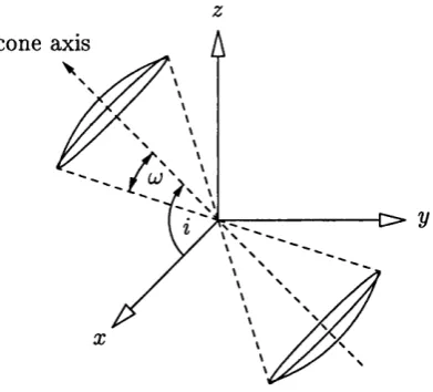
spherical BLR... 41 2.1 A schematic representation of the angular position of clouds in a

right-handed cartesian coordinate system ... 60 2.2 The surface of revolution formed by rotating the sm ooth curve C

about the z -a x is... 61 2.3 The formation of a spherical surface... 62 2.4 T he angular position o f clouds in a right-handed cartesian coordinate

system... 63 2.5 Form ation of a conical surface... 64 2.6 A schematic representation of a disc-shaped BLR geometry inclined

2.10 Model ^ (t;) for an isotropically em itting spherical BLR w ith four different radial velocity laws... 77 2.11 Model for an isotropically em itting spherical BLR and three different radial emission line flux distributions... 78 2.12 The relative positions of the source, cloud and observer in a model BLR... 79 2.13 Model response functions for an isotropically em itting spherical BLR, w ith clouds undergoing gravitational free-fall... 80 2.14 Model r ) for a spherical BLR with four different radial velocity laws... 81 2.15 Model response functions for an isotropically em itting spherical BLR,

w ith clouds moving in randomly inclined circular Keplerian orbits. . 82 2.16 Response function for an isotropically em itting spherical BLR w ith a

chaotic velocity field... 84 2.17 A schematic representation of a bi-conical BLR inclined at an angle

i to the observers line of sight... 85 2.18 Model response function for an isotropically em itting bi-conical BLR. 87 2.19 Model ^ (i;, r ),^ ( i;), and ^ ( r ) for a bi-conical BLR, w ith the same

opening angle b ut w ith different line of sight inclinations... 88 2.20 Formation of the 1-d response function of a disc-shaped BLR... 91 2.21 Model ^ ( r ) for an isotropically em itting thin Keplerian disc w ith three different emission-line flux distributions... 92 2.22 The formation of ^ ( v ) for a disc-shaped BLR... 93 2.23 Model ^ { v ) for an isotropically em itting thin Keplerian disc BLR w ith three different emission-line flux distributions... 94 2.24 Model ^ ( i ;,r ) , W('u) and ^ ( r ) for an isotropically em itting th in Ke­

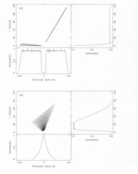
plerian disc BLR w ith differing line of sight inclinations... 95 2.25 Trailed spectrograms, emission-line light-curves, and tim e averaged

line profiles for a variety of BLR geometries and velocity fields. . . . 98 2.26 The corresponding difference spectra, plotted in the form of a trailed

spectrogram for the same BLR geometries and velocity fields... 101 3.1 Variation of the cumulative covering factor C{r) w ith radius r for

3.2 Line and continuum emission line fluxes divided by the local density for steady-state model B ... I l l 3.3 Continua and emission-line fluxes divided by the local density for

steady-state models C -F ... 113 3.4 Emissivity-weighted emission-line response functions for models B -F 121 3.5 Responsivity-weighted emission-line response functions for models B -F 124 3.6 (a) Variation of the emissivity-weighted radius with pressure-law in­

dex s; (b) Variation of the responsivity-weighted radius w ith pressure-law index s ... 126 3.7 Radial variation of the line responsivity distributions for models B -F 129 3.8 Example responsivity-weighted ^ ( r ) for the idealised Case I and Case

II B L R s ... 132 3.9 Variation of the line responsivity distributions as a function of U for

models B - F ... 137 4.1 A schematic representation of clouds in an optically thick BLR. . . . 148 4.2 Form ation of 1-d response functions for anisotropically em itting spher­

ical BLRs... 154 4.3 Form ation of the LIL 1-d response function for an anisotropically

em itting, Case I, spherical BLR... 155 4.4 Form ation of the LIL 1-d response function for an anisotropically

em itting, Case II spherical BLR... 158 4.5 Isotropic and anisotropic response functions for normal case spherical

BLRs... 160 4.6 Isotropic and anisotropic LIL response functions for Case I spherical

BLRs w ith clouds moving in randomly inclined circular Keplerian orbits... 161 4.7 The evolution of ^ (u ) for a Case I, anisotropically em itting, spherical

BLR, w ith clouds moving in randomly inclined circular Keplerian orbits. 162 4.8 Isotropic and anisotropic LIL response functions for a Case II spheri­

cal BLR, with clouds moving in randomly inclined circular Keplerian orbits... 163 4.9 The evolution of for an anisotropically em itting. Case II, spher­

4.10 Isotropic and anisotropic response functions for norm al case spherical BLRs w ith clouds moving in a decelerating radial outflow... 168 4.11 Isotropic and anisotropic LIL response functions for Case I spherical

BLRs w ith clouds moving in a decelerating radial outflow... 169 4.12 Evolution of ^ (î;) for anisotropically em itting, Case I, spherical BLR,

w ith clouds moving in a decelerating radial outflow... 170 4.13 Isotropic and anisotropic LIL response functions for Case II, spherical

BLRs, w ith clouds moving in a decelerating radial outflow... 171 4.14 Evolution of ^ (t;) for an anisotropically em itting. Case II, spherical

BLR, w ith clouds moving in a decelerating radial outflow... 172 4.15 Isotropic and anisotropic response functions for norm al case, bi-conical

BLRs w ith clouds moving in an accelerating radial outflow... 178 4.16 Isotropic and anisotropic LIL response functions for Case I, bi-conical

BLRs w ith clouds moving in an accelerating radial outflow... 179 4.17 Evolution of '^(y) for an anisotropically em itting. Case I, bi-conical

BLR w ith clouds moving in an accelerating radial outflow... 180 4.18 Isotropic and anisotropic LIL response functions for Case II, bi-conical

BLRs, w ith clouds moving in an accelerating radial outflow... 181 4.19 Evolution of for an anisotropically em itting. Case II, bi-conical

BLR, w ith clouds moving in an accelerating radial outflow...182 4.20 Isotropic and anisotropic response functions for a normal case thin

Keplerian disc BLR... 188 4.21 Isotropic and anisotropic LIL response functions for a Case I thin

Keplerian disc BLR... 189 4.22 Evolution of '^{v) for an anisotropically em itting. Case I, th in Kep­

lerian disc BLR... 190 4.23 Isotropic and anisotropic LIL response functions for a Case II, th in

Keplerian disc BLR... 191 4.24 Evolution of for an anisotropically em itting. Case II, th in Kep­

lerian disc-shaped BLR 192

4.25 The F {r) for a number of lines in models B to F ... 193 4.26 1-d anisotropic responsivity-weighted response functions for models

4.27 A comparison of the isotropic and anisotropic responsivity-weighted 1-d response functions for models B, D and F ... 204 4.28 Exam ple anisotropic responsivity weighted response functions for Model

B ... 205 4.29 Exam ple anisotropic responsivity-weighted response functions for model

F ... 206 4.30 Variation of the anisotropic responsivity weighted radius, w ith pres­

sure law index s... 208 5.1 Model steady-state emission line flux distributions plotted as a func­

tion of ionization param eter... 222 5.2 (a) The model continuum light-curve normalized to its mean value.

(b) The fractional change in continuum level from one epoch to the next... 223 5.3 Tim e dependent emissivity-weighted response functions...229 5.4 Model continuum and emission line light-curves for Models I-IV . . . 231 5.5 Variation of the centroid of the instantaneous responsivity-weighted

response function as a function of continuum level for Models I-IV . . 233 5.6 Model non-linear emission-line light-curves... 239 5.7 The variation in Tc as a function continuum level for the instanta­

neous anisotropic responsivity-weighted response functions w ith time- dependent F { r )...245 5.8 Tc versus continuum level for F (r) flxed at the steady-state value. . . 251 5.9 A comparison of the model linear and non-linear emission-line

light-curves for a selection of lines... 254 6.1 Variation in Tg with r... 265 6.2 A schematic representation of a two component BLR... 273 6.3 The 1-d and 2-d response functions and variable line profile for the

separate BLR com ponents... 274 6.4 The 1-d and 2-d response functions and variable line profile of a multi-

B .l B.2

List o f Tables

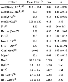
1.1 Continuum and emission-line variability param eters for NGC 5548. . 56

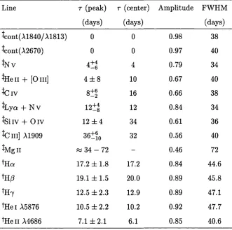
1.2 Cross-correlation results for the continuum and emission-line light-curves of NGC 5548... 57

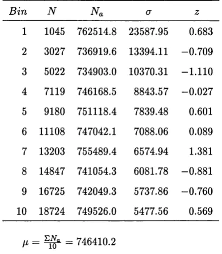
2.1 Results from a test of the randomness of the cloud distribution. . . . 66

2.2 Results of the reduced chi-square te st... 67

3.1 Steady-state param eters for models B - F ... 107

3.2 AGN c o n t i n u u m ... 108

3.3 Integrated emission-line intensities normalized to H/3 for models B -F 117 3.4 The centroids of the emissivity-weighted response f u n c t i o n s ... 119

3.5 The centroids of the responsivity-weighted response functions . . . . 128

4.1 Model response functions centroids for a spherical BLR... 152

4.2 Model response function centroids for a bi-conical BLR... 174

4.3 Model response function centroids for a th in Keplerian disc BLR. . . 183

4.4 The centroids of the anisotropic responsivity-weighted response func­ tions and F factors... 199

5.1 Cross-Correlation Results for Models I-IV ... 234

5.2 Emission line variability param eters...247

C h a p ter 1

A ctive G alactic N uclei

1.1

In tro d u ctio n

the mean fuelling rate w ith time.

1.2

A n h istorical review

Extrem e forms of nuclear activity were first detected in the central regions of (Seyfert) galaxies (Seyfert 1943), Seyferts are generally barred spirals, Hubble type Sb II or Sb III (O sterbrock 1974), with bright compact nuclei, L ~ 10^^ erg s“ ^, which is com parable to the integrated starlight of the surrounding host galaxy. Since the early observations two distinct classes have been identified. Seyfert 1 galaxies display strong broad emission-lines in their spectra (FW ZI ~ 10,000 km s“ ^), indicating fast moving clouds, and emit strongly at ultraviolet and x-ray wavelengths. By con­ trast, Seyfert 2 galaxies display strong narrow lines in their spectra, emit weakly at ultraviolet and x-ray wavelengths, but are strong infra-red em itters.

The development of new observational techniques in the 1950s and 1960s, p ar­ ticularly in the field of radio astronomy led to the discovery of a num ber of elliptical galaxies w ith brilliant nuclei, em itting strongly at radio wavelengths. These radio galaxies can be broadly divided into two sub-classes according to the appearance of their optical spectra (Osterbrock 1974); Broad Line Radio Galaxies (BLRGs) which have broad emission line spectra and emit large am ounts of energy at short wave­ lengths, and Narrow Line Radio Galaxies (NLRGs) which display narrow spectral lines and em it only weakly at short wavelengths. Both classes display narrow jets of m aterial outflowing from their nuclei associated with the strong radio emission, which is assumed to be synchrotron in nature.

emission, although to date most discoveries have been made at optical wavelengths. The last group to be identified were the Blazars, AGN which radiate intensely at all wavelengths and display extreme forms of variability in both their continuum and emission-line intensities, and degree of polarization. This group is sub-divided into Optically Violent Variables (OVVs), which can vary by up to 50% on timescales of less th a n a day and BL-Lacertae objects (BL-Lacs), which have very weak or undetectable emission-lines and vary by factors of 100 or more on timescales of less th a n a few months.

1.3

C lassification

Fanaroff-Riley type I (FRI) or type II (FRII). The former exhibit diffuse, symmetric radio-jets and weakly defined, low luminosity radio lobes. By comparison, FRIIs have well-defined jets and sharp lobe boundaries, high luminosities and bright hot­ spots. A small fraction of radio-loud AGN exhibit extreme forms of activity in the form of rapid variability, unusually high and variable polarization, high brightness tem peratures and compact cores containing gas moving at superlum inal velocities. Collectively known as Blazars, this class of objects is sub-divided into Optically Vi­ olent Variables (OVVs) and BL-Lacertae objects (BL-Lacs), OVVs are essentially type I AGN, which display large am plitude variability (~ 50%) on timescales of a day. BL-Lacs are the most unusual AGN, with extremely weak emission-lines and very rapid high am plitude continuum variability (factor of 100 or more w ithin a few m onths), spanning the full spectral range from radio to 7 -rays. However, the broad sim ilarity in form of the continuum emission for both types of Blazars, suggests th a t they are powered by the same physical processes.

1.3.1

A G N u nification schem es

Unified theories of AGN suggest th a t the various AGN sub-classes are different m anifestations of the same basic phenomenum and th a t apparent differences are caused solely by random orientation effects as opposed to any intrinsic physical difference. There are currently two unification schemes for AGN, one unifying radio­ quiet objects, and the other unifying both radio-quiet and radio-loud objects:

For radio-quiet objects the distinction between type I and type II AGN depends upon w hether the observers line of sight misses or intercepts obscuring m aterial re­ spectively Spectropolarim etric observations of the Seyfert 2 galaxy NGC 1068 (Antonucci & Miller 1985) and the NLRG 3C 234 (Antonucci 1982,1984), both of which display strong broad emission lines in polarized light, supports this general picture. Furtherm ore, observations of light cones in a num ber of type II AGNs, e.g. NGC 1068, NGC 1556 and NGC 3783, also suggests ionization of th e Extended N arrow Line Region (ENLR) gas by a hidden continuum source w ith type I lumi­ nosity. The comparative weakness of the x-ray continuum emission in type II AGN

c.f. type I AGN is also consistent with obscuration of the nuclear emission.

For radio-loud objects, the distinction between the various classes of AGN de­ pends upon differences between the line of sight orientations of their radio-jet axis, which is assumed to be relativistically beamed. Relativistic beam ing not only ex­ plains the rapid variations and high luminosities seen in some Blazars, b ut also explains the preponderance of one-sided radio-jets. Thus, in this scheme Blazars are aligned versions of NLRGs, BL-Lacs are aligned FRIs, and OVVs are aligned SSRQs or aligned FR IIs with BLRGs/SSRQs at interm ediate angles. Surveys of AGN numbers at x-ray and radio wavelengths are consistent w ith this hypothesis (Padovani &: U rry 1990).

1.3.2

A n A G N paradigm

Spectroscopic and photom etric observations of AGN have led to the development of the following generalised picture of these phenomena:

these fuel giant radio-lobes which extend out to several kiloparsecs.

A num ber of plausible theories have been proposed for the apparent dichotomy between radio-loud and radio-quiet objects. One suggestion is th a t all AGN have relativistic jets, b u t those in spiral galaxies are not observed due to dam pening in the interstellar medium by dust. Alternatively, it has been suggested th a t the am ount of radio emission depends upon the rotation rate of the central black-hole, w ith the degree of radio-loudness increasing as the spin rate increases (Blandford 1991). Unfortunately, neither of these theories can as yet be tested observationally.

It should be stressed th a t this model is bu t one of many possible alternatives, whose applicability has yet to be thoroughly scrutinised by observation. Indeed, there is as yet no concrete evidence for the existence of accretion discs and thus no general consensus as to w hether spherical {e.g. see Krolik & London 1983) or disc accretion dom inates the dynamics of the gas close to the central object, although there does appear to be evidence for rotational motion near the central regions of giant elliptical galaxies {e.g. M87).

There is a separate class of objects namely the S tarburst galaxies which display m any of the features characteristic of AGN, for example: strong emission lines, blue continua, strong infra-red emission, and m oderate x-ray luminosities, w ith to tal bolom etric luminosities of ~ 10'^^ erg s“ ^. In some cases this emission arises from an unresolved nucleus. They are generally distinguished by their lack of continuum variability, the absence of strong broad emission lines and most im portantly the appearance of large numbers of ultraviolet absorption lines in their spectra which are associated w ith large numbers of hot massive stars. These objects thus contain dense, localized regions of star formation. These episodes are unlikely to be long lived as there is not enough m aterial to m aintain the high rate of star form ation over the lifetime of the galaxy.

1.4

T h e C entral R egion s O f A G N

de-M BH m o lecu la r torus accretion disc

B L R clo u d s

N L R c lo u d s relativistic je ts

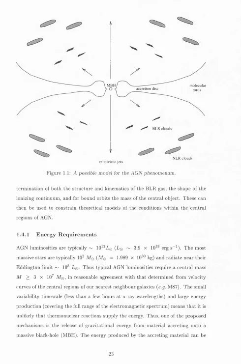
Figure 1.1: A possible model for the AG N phenomenum.

term ination of both the structure and kinematics of the BLR gas, the shape of the ionizing continuum, and for bound orbits the mass of the central object. These can then be used to constrain theoretical models of the conditions within the central regions of AGN.

1.4.1

Energy Requirem ents

AGN luminosities are typically ~ IO^^Lq (Lq ~ 3.9 x 10^^ erg s~^). The most massive stars are typically 10^ M© (M© = 1.989 x 10^^ kg) and radiate near their Eddington limit ~ 10^ L©. Thus typical AGN luminosities require a central mass M > 3 X 10^ M©, in reasonable agreement with that determined from velocity curves of the central regions of our nearest neighbour galaxies (e.g. M87). The small variability timescale (less than a few hours at x-ray wavelengths) and large energy production (covering the full range of the electromagnetic spectrum) means th a t it is unlikely th at thermonuclear reactions supply the energy. Thus, one of the proposed mechanisms is the release of gravitational energy from material accreting onto a massive black-hole (MBH). The energy produced by the accreting material can be

expressed as

L = jiM c^ , (1.1)

where /x represents the accretion efl&ciency {i.e. the fraction of the mass converted into gravitational energy), M is the accretion rate, and c is the velocity of light. For typical AGN luminosities, M ~ 0.7 M© y r“ ^, assuming an accretion efficiency of

~ 10%.

1.4.2 M ass E stim a tes

T he mass of the NLR can be estim ated from simple case B recom bination theory. Assuming th a t each hydrogen ionizing continuum photon ultim ately results in the production of at least one H/? photon, the observed intensities of H/3 in the most luminous Seyfert 2 galaxies and NLRGs (L(H ^) ~ 10®L©) imply masses for the ionized gas of ~ lO^M© (assuming a spherical cloud distribution. Ne ~ 10^cm~^, and a filling factor of ~ 1%) at radial distances of ~ 10^ parsecs. This size estim ate is in good agreement with the observed extent of the NLR gas in those objects in which the NLR has been resolved (~ 10^-10^ parsecs) and is consistent w ith the absence of observed variability in the narrow emission lines.

Similar argum ents suggest th a t the mass of ionized gas in the BLR ranges from between ~ IM© for the lowest luminosity objects, up to a few tim es lO^M© at the high luminosity end (assuming a spherical cloud distribution. Ne ~ 10^ cm “ ^, and a volume filling factor of 1%), w ith corresponding sizes of between a few light-days up to a few light years. These size estimates are also in reasonable agreement with the observed variability timescales of both high and low luminosity AGN.

1.5

Ion izin g con tin uu m sh ape

Defining the shape of the ionizing continuum is crucial to the success of photoioniza­ tion models of the BLR. Although the precise form of the spectral energy distribution differs am ongst different AGN sub-classes, there are a large num ber of similarities. For example, all AGN display an intense featureless continuum which may be ap­ proxim ated by a powerlaw over a limited range in frequency such th a t

where ^ is the observed flux of ionizing photons (erg cm “ ^ s“ ^ and a is the spectral index. U nfortunately the most im portant part, the Lym an continuum up to soft x-ray energies is not observed, except in some high redshift quasars, where in- tergalactic absorption by low column density gas (in the form of b o th line blanketing and Lym an-lim it discontinuities) severely depresses the continuum and subsequently hinders an accurate determ ination of the continuum shape in this region. Thus in­ direct m ethods must be employed to determine in this gap.

For bo th radio-loud and radio-quiet quasars, the near infra-red continuum (1 — 3//m) is well-fitted by a single powerlaw with a; ~ 1 — 2 (Neugerbauer et a l 1979; Elvis et a l 1986; Edelson & Malkan 1986; Neugerbauer et a l 1987; Carleton et a l 1987), w ith an additional small bum p at around 3.5//m due to therm al emission from dust grains in the vicinity of the BLR (Hyland & Allen 1982; Edelson & Malkan 1986; Carleton et a l 1987; Barvainis 1987), although free-free emission from dense clouds near the BLR (P uetter &: H ubbard 1985) or from the optically- th in region of an accretion disc (Collin-Souffrin 1987b) may also contribute. The shape of the infra-red continuum is of particular im portance since free-free infra­ red emission can provide a significant heat-source for the BLR gas, which may drastically affect the line emission, particularly of collisionally excited lines (Ferland et a l 1992). However, the lack of observed variability in the infra-red relative to variations in the other continuum bands (Neugerbauer et a l 1979; Glass 1981; C utri et a l 1985; Sembay, Hanson & Coe 1987) suggests th a t this component is produced in an extended region external to the BLR, and thus has a negligible heating effect upon the BLR clouds.

emission and numerous blended Fe ll lines (Oke, Shields & Korycansky 1984; Wills, Netzer & Wills 1985).

At shorter wavelengths the continuum m ust tu rn over in order to connect the optical-ultraviolet and soft x-ray continuum (Kinney et al. 1985, Wilkes & Elvis 1987). O ’Brien et al. (1987) estim ate a change in spectral index A a ~ 1, giving a mean slope in the far ultraviolet of ~ 1.4, similar to th a t derived by Czerny and Elvis (1987) for a variety of accretion-disc models. This, together w ith the strong correlation found for the near infra-red (3.5/zm) and hard x-ray (2keV) continuum luminosities in Seyferts, quasars and Blazars (Glass 1979; Kriss, Canizares &; Richer 1980; Lawrence &: Elvis 1982; Malkan 1984, 1985) suggests th a t a single com ponent w ith slope 1.4 extending from the infra-red to soft x-rays underlies the optical- ultraviolet continuum.

A num ber of objects show an excess of emission at ultra-soft x-ray energies (0.1 — 0.28 KeV) relative to the extrapolation of the infra-red continuum into the x-ray region (A rnaud et al. 1985; Branduardi-Raym ont et al. 1985; Wilkes &: Elvis 1987; Turner & Pounds 1989; Gondhalekar 1994) which displays rapid variability. In a few AON this excess extends up to a few keV, forming a ‘soft x-ray excess’ (Bechtold et al. 1987a). The ultra-soft and soft x-ray excesses, which are thought to be produced in an electron scattering atmosphere, are rarer in BL-Lac objects and may therefore be associated with the high-energy tail of the ‘big blue b u m p ’, which is not observed in BL-Lacs.

The shape of the high energy tail {E > 30 keV) is fairly uncertain, and has been observed in only a few objects. Ginga x-ray observations of Seyfert 1 galaxies (Pounds 1990) show strong Fe Ko; emission and a broad hum p at energies > 10 keV. A possible production mechanism for the high energy tail is the reflection of power-law x-rays (o; ~ 0.9) by cold (T ~ 10^ K) m atter (G uilbert Sz Rees 1988; Lightm an & W hite 1988).

of different continuum emission processes at various orientations. Furtherm ore, the ‘big blue b u m p’ appears to be significantly weaker in the optical and ultraviolet (A > 1200 Â) for lower luminosity Seyfert 1 galaxies and quasars (Malkan Sz Sargent 1982; Kriss 1988), whilst BAL quasars and blazars have steeper optical-ultraviolet continua th an quasars (O ’Brien et al. 1987a; Malkan & Stockman 1984; Ghisselini et al. 1986), which may also be a result of the dominance of different continuum processes in the former relative to the latter (Stein Sz O ’Dell 1985). Additionally, x-ray observations indicate th a t the soft x-ray continuum hardens w ith increasing radio-loudness (Zamorani et al. 1981). Assuming a powerlaw fit to the x-ray contin­ uum , the spectral index in the 0.1 — 3.5 keV region is o; ~ 0.5 for radio-loud quasars com pared to a % 1.0 for radio-quiet quasars (Wilkes Sz Elvis 1987) indicating th a t synchrotron self-compton emission dominates the x-ray in radio-loud quasars. By contrast, 2 — 10 keV slopes of 0.7 ± 0.15 were found for radio-quiet Seyfert 1 galax­ ies (M ushotzky et al. 1980, M ushotzky 1984) which suggests a flattening of the continuum at shorter wavelengths in radio-quiet objects.

It has been suggested th a t the shape of the EUV to soft x-ray continuum may be inferred by comparing the observed emission-line intensities w ith those deduced from photoionization calculations {e.g. see Kwan 1986; Bechtold et al. 1987a; Netzer 1987). However, continuum sensitive lines are generally at least as sensitive to other physical param eters such as density, column density and ionization param eter and thus only very general constraints can be placed. A b etter understanding of the optical F ell emission may provide some inform ation on the shape of the ionizing continuum , as the strength of the optical Fe II lines appears to correlate with otox in the sense th a t objects w ith flatter x-ray spectra {i.e. smaller aox) have weaker optical F ell emission (Wilkes, Elvis & McHardy 1987; Zheng & O ’Brien 1990), whereas photoionization calculations would tend to suggest the opposite correlation (Netzer 1987; Krolik 1987).

1.5.1

D u st in A G N s

and emission-line intensities.

For the NLR, estimates of the am ount of dust extinction are found by comparing the observed Balmer line ratios (typically 6) with those determ ined from photoionization calculations (H a/H /?~ 3.1). These are consistent w ith m oderate degrees of reddening. Note th a t the model value differs from the case B recombi­ nation value of 2.8 because Ho; is collisionally de-excited. Furtherm ore, the strong blue asym m etry of the narrow lines in AGN is consistent w ith dust obscuration in optically thick radially moving clouds. For the BLR the Balmer line ratios cannot be used as b oth collisional excitation and optical depth effects result in line ratios which are far from their simple case B values. Instead the ratios of those lines which originate from the same upper level, and which are thus less susceptible to collisional excitation effects, are used {e.g. P a / H a and P /)/H ^ ). Lines w ith well de­ term ined theoretical line ratios have also been used to estim ate the am ount of dust extinction {e.g. H ell A1640/Hell A4686 (MacAlpine 1981; Netzer 1991; K oratkar k, MacAlpine 1992), and O l A1302/OI A8446 (Netzer k Davidson 1979; MacAlpine k Feldm an 1982). A comparison of these line ratios w ith photoionization calculations also indicate m odest am ounts of reddening { Eb-v ~ 0.2). Furtherm ore, the ratios

of the ultra-violet lines w ith respect to Lyo: are generally in b etter agreement w ith photoionization calculations th an the op tical/L ya line ratios, which is also consis­ ten t w ith extinction by dust, although there are alternative explanations {e.g. a two com ponent BLR).

1.6

T h e B road Line R egion o f A G N

Here the structure and physical conditions within the BLR, as determ ined through b o th spectroscopic and photom etric studies in combination w ith photoionization modelling techniques, is described.

1.6.1

C overing factor

For low luminosity AGN, the covering factor {i.e. th e fraction of sky, as seen from the ionizing continuum source, th a t is covered by BLR clouds) is usually estim ated from the equivalent w idth of Ho;. Assuming th a t each ionizing continuum photon ultim ately results in the production of at least one H a photon, then observations suggest covering factors in the region of 10-50%. M ushotzky and Ferland (1984), argued th a t x-ray absorption suggests covering factors near unity for Seyfert 1 galax­ ies, although more recent x-ray observations dispute this (Gondhalekar et al. 1994; Gondhalekar 1994). For high luminosity AGN, the covering factor can be estim ated from the drop in the continuum level ju st shortward of the Lyman limit (Sm ith et al. 1981; MacAlpine & Feldman 1982; K oratkar et al. 1982). An observed drop of 0.1 in continuum intensity shortward of A912Â, suggests optical depths r(912Â ) <C 1 if the continuum source is completely obscured. However, the presence of strong broad M gll and F ell lines in AGN spectra suggest much larger optical depths, and thus covering factors of ~ 10 percent.

1.6.2

C olu m n d en sity

The column density is estim ated at between 10^^ — 10^^ cm~^. The lower limit is set by the appearance of low excitation lines of M gll and F ell in AGN spectra, whilst the upper limit is set by observations of Ca II in some AGN spectra (Ferland k. Persson 1989; Van Groningen 1993).

1.6.3

C h em ical A bundances

to hydrogen are ill-determined due to uncertainties in the calculated intensities of the hydrogen lines. A comparison of the observed emission-line intensities of AGN w ith intensities calculated from photoionization models suggest th a t the chemical com position of the BLR and NLR gas is similar to th a t found in our own galaxy, and galaxies w ith H II regions or bursts of star formation, w ith the possible exception of nitrogen which appears to be overabundant by a factor of 5 (Osmer & Sm ith 1976), and helium which is overabundant by a factor of 1.4 relative to cosmic abundances (O sterbrock 1989).

1.7

P h o to io n iz a tio n m od els o f th e B L R

O ur current understanding of the physical conditions within the BLR have been deduced from measurements of the line intensities of a large num ber of Seyfert 1 and quasar spectra combined with theoretical models of the line-emitting gas. As noted by Seyfert (1943), the spectra of AGNs display many of the lines typical of a classically photoionized nebula. Consequently, there exists a strong historical link between the early BLR models and photoionization models of galactic nebulae. T he earliest models, which can be dated back to the work of Bahcall and Kovlovski (1969), Davidson (1972), and MacAlpine (1972), were an attem p t at determ ining the excitation mechanism of the BLR gas, and other general physical properties {e.g. chemical composition, density, and column density).

S tandard ‘single cloud’ models of the BLR used today are characterized by the shape of the hydrogen ionizing continuum, usually taken to be a powerlaw in fre­ quency, Fjy oc (where a is the spectral index), the hydrogen density a t the ionized face of a plane-parallel slab of gas N , and an ionization param eter U, a dimensionless quantity representing the ratio of photon to m atter density, w ritten here as

penetrating x-rays heat the gas, m aintaining a partially ionized zone which em its strongly in the low ionization lines (LILs) {e.g. Balmer lines, M gll and F ell) and Balmer and Paschen continua.

The absence of an observed cut-off at the Lyman limit in a large num ber of high redshift quasars, imply th a t the fraction of the sky covered by BLR gas is small (~ 10%), bu t may be larger in Seyfert 1 galaxies (Smith et al. 1981). Also, the observed intensities of the emission-lines indicate th a t the volume filling fraction of the line em itting m aterial is very small (10“ '^). This, together w ith the absence of stru cture in the observed emission-line profiles imply th a t the BLR is made up of a large num ber of small high velocity clouds which intercept only a small fraction of the to tal ionizing continuum and occupy only a small fraction of the available space.

The observed ratios of the C ill] A1909 and CIV A1549 lines relative to L y a A1215 are similar in objects covering a wide range in luminosity, implying th a t the BLR gas exists w ithin a very narrow range of physical conditions. The tem perature, as deter­ mined from the ratio of the C m ] A977 / Cill] A1909 lines is ~ K, insufficient to produce the high degree of ionization seen in BLR spectra through collisional excita­ tion, and further evidence th a t photoionization is the main energy source. Density limits are set by the absence of strong broad forbidden lines such as [O ill] A4363 which are collisionally de-excited at low densities ~ 10^ cm~^, and by the presence of strong broad C m ] A1909, an intercombination (or semi-forbidden) line which is col­ lisionally de-excited at densities above 10^^ cm~^ (Davidson &: Netzer 1979). Large Lym an continuum optical depths are required to account for b o th the streng th of broad M gll and to fit the observed F ell emission-line spectrum (Phillips 1978; Wills, Netzer & Wills 1985). Observed ratios of the ultraviolet to optical F ell lines indicate optical depths ( r > 10^).

S tandard photoionization models assuming values of f7 ~ 0.01, and N ~ 10^^ cm~^, reproduce the observed intensities of the strongest ultra-violet lines relative to each other and to Lyo; A1215 w ithin a factor of a few. Re-arranging equation 1.3, yields a characteristic ‘size’ for the BLR of

r = 63 X light-days , (1.4)

w h e re Q s i i h ) is th e n u m b er o f h y d ro g en io n izin g p h o to n s s~^ in u n its o f 10^'^, N i o

ionization param eter in units of 0.01, which for typical Seyfert 1 galaxy and quasar luminosities and standard BLR param eters gives a radius of ~ 100 light-days for Seyfert 1 galaxies (Qs4(A') ~ 1) and ~ a few parsecs for quasars 100).

Despite its apparent success, the standard model of the BLR does have a num ­ ber of problems. In particular, models with standard BLR param eters produce steep Balmer decrements (L y a/H /l ~ 50, H a/H jd ~ 10) (Davidson h Netzer 1979), whereas the mean observed values are far lower (Lya/H/3 ~ 3, Ho;/H/? ~ 4) (Baldwin 1977a). In addition, standard models produce far less emission in the Balmer contin­ uum and Fe ll lines th an is typically observed, the so-called ‘energy budget problem ’ (Netzer 1985; Collin-Souffrin 1986). Models invoking high densities, high column densities and m oderate degrees of ionization can produce lower Balmer decrements, b u t the higher densities involved result in weaker th an observed C III] emission (Fer­ land k, Persson 1989). The standard model of Kwan and Krolik (1981), produces lower Balmer decrements by invoking strong heating by x-rays at large column den­ sities. This produces an extended partially ionized zone which emits strongly in the Balmer lines, Fe ll lines and Balmer continuum. However, this model has been crit­ icized because the ratio of the energy in the x-ray to ultraviolet continuum ( ~ 10) is far larger th an is typically observed (Netzer 1987).

A nother m ajor uncertainty in photoionization calculations is the degree of red­ dening of the observed spectrum . A heavily reddened continuum could help solve the energy budget problem, giving a much flatter spectral index th a n is typically observed (Netzer 1985). However, it is unlikely th a t dust grains could survive in th e radiation pressure and tem peratures found w ithin the BLR.

general redshifted with respect to the HILs in many objects (Gaskell 1982; Shuder 1982; Wilkes 1984; Wilkes 1986).

1.7.1

T h e io n ization stru ctu re o f o p tica lly th ick and o p tic a lly th in

clouds

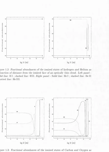
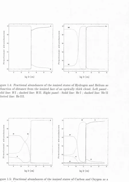
To illustrate the difference between the internal ionization structure of an optically thick and an optically thin cloud, Figures 1.2—1.5 show the fractional abundances of the ionized states of hydrogen, helium, carbon and oxygen as a function of distance from the ionized face of the cloud.

The predicted emission-line spectrum from a uniform slab of gas at a radial dis­ tance r from an ionizing source of continuum radiation was calculated using the photoionization code CLOUDY, version 80.06c (Ferland 1991, 1993). The detailed physics involved in com puting the emission-line spectrum has been discussed else­ where (Davidson & Netzer 1979; Kwan h Krolik 1981; Rees, Netzer &: Ferland 1989; Ferland 1991), and will not be repeated here.

The incident ionizing continuum is taken as CLOUDY’s ‘Table AGN’ option, similar to th a t described by M atthews and Ferland, and typical of a radio-quiet AGN. The sub-millimeter break was set at 10/xm, and for longer wavelengths the continuum has the form Fy oc Integrating over frequency yields a mean photon energy hv = 3.038 Rydberg for this continuum. The cloud density and column density were set at 10^® cm~^ and 10^^'^^ cm“ ^ respectively. Individual clouds were chosen to have constant density, although constant pressure clouds are found to give similar results. The chemical composition was taken to be solar, w ith abundances taken from Grevesse and Anders 1989. For the optically thick cloud, U = 0.01 whilst for the optically thin cloud, U = 10.0, which is equivalent to a thousand fold increase in the incident flux of ionizing photons over the optically thick model. This yields an optical depth at threshold for Lyo; of % 3.4 x 10® in the optically thick model, and % 0.8 in the optically thin model.

1.7.1.1

Optically thin clouds

u 0.8

1.0

0.8

0.8

0.4

0.0

I 10 11 12 13 14

log ôr (cm) log ôr (cm)

Figure 1.2: Fractional abundances o f the ionized states o f hydrogen and Helium as a function o f distance from the ionized face o f an optically thin cloud. Left panel -Solid line: H I ; dashed line: H II. Right panel - Solid line: He I ; dashed line: He II : dotted line: He III.

1.0

0.8

0.8

0.4

Q2

0.0

» 10 11 12 13 14

1.0

Oi

0.8

0.4

02

0.0

9 10 11 12 13 14

log ôr (cm) log ôr (cm)

Figure 1.3: Fractional abundances o f the ionized states of Carbon and Oxygen as a function o f distance from the ionized face o f an optically thin cloud. Left panel - Solid line: C IV ; dashed line: C V ; dotted line: C V I; dot-dashed line: C V II. Right panel - Solid line: O III & O Vll ; dashed line: OIV & OIX ; dotted line: O V

Helium (Figure 1.2, right panel) is predom inantly He^+, with a small contribution from He"^ beyond the He'*' — He^+ ionization edge formed near the back-face of the cloud. In an optically thin cloud the m ajority of the cooling is performed by the high ionization lines, for example, the higher states of carbon and oxygen. Due to the large ionization param eter multiple Strom gren spheres of carbon and oxygen are formed, w ith the highest ionization states effectively shielding the lower states from the most intense radiation. For such clouds, the fractional abundances of the lines are relatively independent of the ionization param eter (Ferland &: Persson 1989).

In theory, for clouds w ith the same density and column density, ionized by a continuum w ith the same spectral energy distribution, the Strom gren length 8r is directly proportional to the flux of ionizing photons 0 , such th a t 6r =

where a is th e recombination coefficient (Osterbrock 1974). Hence the ionization stru cture should in principle scale linearly w ith U. This is not the case here due to the large difference in the ionization param eter, 3.0 in dex, and the absence of the hydrogen ionization edge in the optically th in model.

An im po rtant question to resolve is whether or not clouds located in such an intense radiation field are stable against disruption by radiation pressure. For the optically th in cloud, the internal radiation pressure dominates the gas pressure for lo g 6r > 12.3 (position of the ionization edge). This cloud is therefore unstable to disruption by radiation pressure if supported by an external m edium alone. However, this is not a problem if some other mechanism, such as m agnetic pressure, provides the support (Rees 1987).

1.7.1.2

Optically thick clouds

1.0

0.8

0.0

0.4

0.0

0 10 11 18 13 14

log ôr (cm) log ôr (cm)

Figure 1.4: Fractional abundances of the ionized states of Hydrogen and Helium as a function o f distance from the ionized face o f an optically thick cloud. Left panel - Solid line: H I ; dashed line: H II. Right panel - Solid line: He I ; dashed line: He II ; dotted line: He III.

1.0

0.8

0.6

0.4

0.0

0 10 12 13 14

log ôr (cm) log ÔF (cm)

mostly and oxygen mostly although there are small fractions in th e form of and 0^+. This optically-thick cloud is stable as the gas pressure dom inates the radiation pressure at all radii.

1.8

V ariab ility S tu dies — C h allen gin g th e S tan d ard

M o d el

Recently a potentially more serious problem has been identified. In a num ber of objects the continuum and broad emission-lines are seen to vary on relatively short timescales {e.g. see the review by Peterson 1993). Light crossing argum ents im ply th a t the size of the BLR as derived from the observed variability is up to an order of m agnitude smaller th an th a t predicted by standard models. If the observed values of U are correct, this implies much larger densities th an previously thought, conversely, if the densities are correct, higher ionization param eters are required. At least some gas w ith larger U values is necessary to produce the observed strength in O VI A1035 and N v A1240. A plausible model for the BLR is one in which the BLR gas exists over a broad range of physical conditions, and an observer thus sees an average over gas of very different properties.

1.8.1 T h e P o in t Source R everb eration M od el o f th e B L R

The widely accepted explanation for the observed broad emission-line variations is generally expressed in term s of the point-source reverberation model of the BLR. In this model emission-line clouds are assumed to be linear reprocessors of con­ tinuum radiation and to respond instantaneously to variations in the intensity of the ionizing continuum. The response of the BLR clouds to continuum variations are therefore assumed to be dominated by light travel-time effects w ithin th e BLR. T he assum ption of linearity is addressed in C hapter 5. The instantaneous response approxim ation may be justified through a careful consideration of the following fun­ dam ental timescales:

(i) R e c o m b in a tio n tim e

"

aJVe ’

(15)

where a is the recombination coefficient, and iVg is the electron density. For typical BLR densities (jVg ~ 10^® cm“ ^) the recombination tim e for hydrogen is ~ 10^ seconds, far smaller th an any line variation yet observed.

(ii) D y n a m ic a l tim e

A nother im portant timescale is the dynamical tim e t^yn for the BLR, which is th e am ount of tim e taken for a cloud to cross the BLR, or for bound orbits, the orbital period of a BLR cloud. The dynamical time is related to the mean BLR size r, and m ean cloud velocity v, by

T

^dyn ~ Z ' (1 6)

Cross-correlation estimates of the BLR size are typically a factor of ten times smaller th a n th a t derived from photoionization calculations (Gaskell Sz Sparke 1986; Zheng et a l 1987; Gondhalekar 1987,1988,1989; Peterson 1993). However, estim ates of the BLR size from cross-correlating continuum and emission-line light-curves are particularly sensitive to the line species under consideration, and for geometrically thick BLRs are heavily biased toward the inner regions (Edelson Sz Krolik 1988; Robinson & Pérez 1990). Hence, the average BLR radius used here is th a t derived from standard photoionization models of the BLR, noting th a t at most the answer derived here will be out by a factor of ten in f . For standard BLR param eters {i.e. U = 10“ ^ and N = lO^o cm “ ^), the BLR radius f of a typical Seyfert 1 galaxy is ~ 10^® cm (luminosity lO^^ erg s“ ^, < hv >= 3.0 Rydberg). The m ean cloud velocity is typically 10^ km s“ ^, giving a dynamical time, tdyn ~ 10^ seconds. This is considerably larger th an the typical continuum variability timescale (days-m onths), and suggests th a t the BLR is stable on timescales of a few tens of years.

(iii) S o u n d c ro s s in g tim e

ts c = — ,

(1.7)

where Cs = ^j2kTe/'mp. The total thickness of an individual BLR cloud is not well defined, b u t estimates of the extent of the ionized gas (from standard photoionization calculations) are in the region of 10^^ —10^^ cm. For typical cloud radii and electron tem peratures (Tg ~ 10^ K), the sound crossing time, tgc — 10® — 10® seconds. Again this is much larger than the observed continuum variability timescale.

(iv) P h o to n d iffu sio n tim e s c a le

T he photon diffusion timescale is a measure of the time taken for a line photon to escape from the cloud in which it was formed. Lines with low optical depths escape on timescales of ~ R s/c, where Rs is the Stromgren radius. For resonance-lines or lines w ith large optical depths, e.g. Lyo the diffusion time is approxim ately 20 times the direct light-travel time through one Stromgren depth (Hummer k, K unasz 1980), i.e.

I'diff ~ 20i?s/c % 2QUINeOiB , (1 8 ) where U is the ionization param eter, iVg the electron density, and o # i s the Menzel- Baker case B recombination coefficient. For the conditions thought to exist w ithin the BLR, Rs ~ 10^^ cm (Peterson 1994) and thus t^ iff ~ a few minutes. Thus the photon diffusion timescale is only im portant for high column density, high U clouds, or for lines w ith very large optical depths.

(v) C lo u d re s p o n s e tim e s c a le

(vi) C lo u d fo r m a tio n tim e s c a le

The cloud formation timescale is highly model dependent requiring basic theoretical assum ptions concerning the origin of the BLR gas. Perry and Dyson (1985) produced a self-consistent model wherein BLR clouds are formed behind radiative shocks around obstacles in the interstellar medium (see also Dyson, Williams, Sz Perry 1994; Perry 1994). In their model the cloud formation timescale (or equivalently the cooling time) of the post-shocked gas is ~ a year. The lifetime of the clouds is of the order of the flowtime around the obstacles (typically a year to a few tens of years). This suggests th a t the BLR changes its structure on dynamical timescales and th a t differences will be found in both profiles and response functions on timescales longer th a n this.

Assuming th a t the line em itting gas responds instantaneously to continuum varia­ tions, the am ount of information th a t can be gleaned using variability techniques depends upon two further timescales: (a) the light-crossing time, and (b) the con­ tinuum variability timescale.

(a) L ig h t-c ro s s in g tim e

The light-crossing time determines how quickly continuum variations cause changes in the line profiles. In order to determine the velocity field of the BLR, the light-crossing time Îlt ^ tree, otherwise the BLR would respond on the recom bina­

tion tim e scale making it impossible to determine the velocity field. (b) C o n tin u u m v a r ia b ility tim e s c a le

The continuum variability timescale tyar, is defined as the time taken for significant changes in the continuum flux to occur. If tyar then the line intensities are always directly proportional to the continuum intensities, and there would be no detectable variation in the line profile, other th an an overall scaling of line inten­ sity w ith continuum luminosity. If however tyar the continuum variations are so rapid th a t only a geometrically thin BLR reflects the continuum level at a given epoch. For a geometrically thick BLR, the line response is an average over gas responding to continuum variations at previous epochs, and the response to a particular continuum event is effectively smoothed out.

in

o u t

t o o b s e r v e r

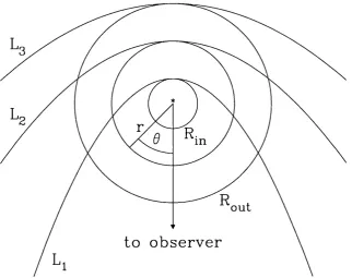
Figure 1.6: A schematic diagram depicting the passage o f light-fronts through a spherical B L R o f inner radius Rin and outer radius Rout- E^ch parabola represents a slice through a surface o f constant time-delay r , where r = r / c ( l — cos 6).

timescale w ithin the BLR, then a cloud located at position {r,6), will be seen to respond at tim e ti to a delta-pulse change in the continuum level at tim e to after a time-delay r = ti — to = r /c { l — cosû). For a geometrically thick BLR, th e locus of clouds on a given iso-delay surface describes a paraboloid. Figure 1.6 shows a section through a spherical BLR of inner radius Rin outer radius Rout, and three different light-fronts labelled L i, L2 and L3. L \ corresponds to a time-delay r = 2 x Rin/c^

L2 corresponds to r = {Rin + Rout)/c and L 3 corresponds to r = 2 x Rout I

/

'^ {v ,r )C { t - t ) dr , (1.9)

-oo

where is w hat is variously known as the emissivity-weighted 2-d ‘response function’, ‘transfer function’ or ‘echo image’ (Blandford & McKee 1982), Im posing causality, in the sense th a t the continuum variations are assumed to drive the line variations and not vice versa, implies th a t ^ ( i ;,r ) = 0 for r < 0, and thus 1,9 can be rew ritten as:

roo

L {v ,t) = / — t ) dr . (1,10)

Jo

^ (i), r ) is a projection of the BLR 6-dimensional phase space (3 spatial, and 3 veloc­ ity) into 2-dimensions, and thus contains essentially all the inform ation necessary to deduce the BLR geometry and kinematics. Thus, the aim of reverberation m apping is to m onitor continuum and emission-line profile variations in an attem p t to re­ cover and thereby determine the geometry and kinematics w ithin the BLR, either by inverting equation 1,10 using fourier techniques and solving for ^ ( v , r ) directly {e.g. see Blandford & McKee 1982, Maoz et al. 1991), or by finding a solu­ tion for '^{v,t) th a t best fits the continuum and emission-line variations {e.g. th e

m axim um entropy m ethod). Due to the absence of regularly sampled, high signal- noise, high resolution spectra, only one serious attem p t has been made at recovering ^(-u, r ) (Krolik &; Horne 1991), Instead attention has focused on recovering the 1-d response function ^ ( r ) from monitoring variable continuum and emission-line intensities. In 1-d equation 1,10 reduces to

roo

L{t) = / ' ^{t) C {î - t) d r . (1,11)

Jo