Nat. Hazards Earth Syst. Sci., 11, 2617–2651, 2011 www.nat-hazards-earth-syst-sci.net/11/2617/2011/ doi:10.5194/nhess-11-2617-2011
© Author(s) 2011. CC Attribution 3.0 License.
Natural Hazards
and Earth
System Sciences
Rockfall characterisation and structural protection – a review
A. Volkwein1, K. Schellenberg2, V. Labiouse3, F. Agliardi4, F. Berger5, F. Bourrier6, L. K. A. Dorren7, W. Gerber1, and M. Jaboyedoff8
1WSL Swiss Federal Institute for Forest, Snow and Landscape Research, Z¨urcherstrasse 111, 8903 Birmensdorf, Switzerland 2Gruner+Wepf Ingenieure AG, Thurgauerstr. 56, 8050 Z¨urich, Switzerland
3Swiss Federal Institute of Technology Lausanne EPFL, Rock Mechanics Laboratory LMR, GC C1-413 Station 18, 1015 Lausanne, Switzerland
4Universit`a degli Studi di Milano-Bicocca, Dip. Scienze Geologiche e Geotecnologie, Piazza della Scienza 4, 20126 Milano, Italy
5Cemagref, Mountain Ecosystems and Landscapes Research, 38402 Saint Martin d’H`eres Cedex, France 6Cemagref, UR EMGR, 2, rue de la Papeterie, BP 76, 38402 Saint Martin d’H`eres Cedex, France
7Landslides, Avalanches and Protection Forest Section, Federal Office for the Environment FOEN, Bern, Switzerland 8University of Lausanne, Institute of Geomatics and Analysis of Risk, Amphipole 338, 1015 Lausanne, Switzerland Received: 25 March 2011 – Revised: 26 July 2011 – Accepted: 7 August 2011 – Published: 27 September 2011
Abstract. Rockfall is an extremely rapid process involving long travel distances. Due to these features, when an event occurs, the ability to take evasive action is practically zero and, thus, the risk of injury or loss of life is high. Damage to buildings and infrastructure is quite likely. In many cases, therefore, suitable protection measures are necessary. This contribution provides an overview of previous and current research on the main topics related to rockfall. It covers the onset of rockfall and runout modelling approaches, as well as hazard zoning and protection measures. It is the aim of this article to provide an in-depth knowledge base for researchers and practitioners involved in projects dealing with the rock-fall protection of infrastructures, who may work in the fields of civil or environmental engineering, risk and safety, the earth and natural sciences.
1 Introduction
Rockfall is a natural hazard that – compared to other haz-ards – usually impacts only small areas. However, the dam-age to the infrastructure or persons directly affected may be high with serious consequences. It is often experienced as a harmful event. Therefore, it is important to provide the best possible protection based on rigorous hazard and risk man-agement methods. This contribution gives an overview of the assessment on parameters needed to deal effectively with
Correspondence to: A. Volkwein
a rockfall event from its initiation to suitable protective mea-sures. This includes a presentation of typical applications as well as an extensive literature survey for the relevant topics that are evaluated and discussed with regard to their perfor-mance, reliability, validation, extreme loads, etc. Contribu-tions include
– Rockfall susceptibility together with hazard assessment and zoning.
– Rockfall initiation and runout modelling
– Design and performance evaluation of rockfall protec-tion systems, with particular attenprotec-tion paid to structural countermeasures such as fences, walls, galleries, em-bankments, ditches or forests
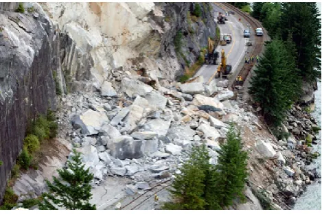
Fig. 1. Rockfall on Sea to Sky highway (B.C.). Note the jointed
structure of the source area (Canadian Press photos).
During the night of 29 July 2008, a rockfall blocked the high-way Sea to Sky joining Vancouver to the ski resort Whistler (Fig. 1). This road is the cover picture of the well-known rock mechanics book by Hoek and Bray (1981). The area has been extensively investigated for risk analysis in the past (Bunce et al., 1997) and still is, because of an increase in population density (Blais-Stevens, 2008) and the Olympics Games in 2010.
Further difficulties exist when the goal is to assess risk (or hazard) on a regional scale for a limited area or over an entire territory. Generally, inventories exist only in inhabited areas. Moreover, some studies suggest that the number of events in-creases in proportion to urbanization (Baillifard et al., 2004). As a consequence, it is necessary to find ways that allow one to detect rockfall hazard source areas in the absence of any inventory or clear morphological evidence, such as scree slopes or isolated blocks.
This article is structured following the typical work-flow when dealing with rockfall in practice (Vogel et al., 2009), covering rockfall occurrence and runout modelling approaches, hazard zoning and protection measures.
When a rockfall hazard or risk analysis (including the pro-tective effect of forests) reveals a threat to people, buildings or infrastructures (see Sect. 2), suitable structural protection measures have to be selected according to the expected event frequency and impact energies. For proper design and di-mensioning of the measures, it is essential to know the mag-nitude of the impact loads and the performance of the struc-tures. This knowledge can be obtained from rockfall onset susceptibility/ hazard analysis, numerical simulations, exper-iments, models or existing guidelines, and provides guidance on the design of roof galleries, fences, embankments and forests as a natural protection system.
However, rockfall protection considerations involve not only structural protection measures but also the avoidance of infrastructure or buildings in endangered areas. Firstly, it
has to be clarified why and where rocks are released and the total volume or extent. The rockfall initiation also depends on different factors, mostly not yet quantified, such as weath-ering, freezing/melting cycles or heavy rainfall (see Sect. 3). Subsequent trajectory analyses determine the areas that have to be protected by measures. To account for their high sensi-tivity to just small changes in the landscape, such as bedrock, dead wood, small dips, etc., stochastic analyses are usually performed, preferably including an evaluation of the accu-racy of the results. This is described in more detail in Sect. 4. However, for a quick preliminary analysis and estimation of the rockfall hazard, simpler and manual calculation methods might also be useful as described in Sect. 4.4.1.
There is a large variety of structural protection measures against rockfall. These include natural protection by means of forests, semi-natural structures such as embankments and ditches and fully artificial structures such as fences, galleries or walls. The structural part of this contribution focuses mainly on fences and galleries. A short summary for em-bankments is also given. Natural protection by means of forests is mentioned in Sect. 5.5.
2 Rockfall hazard: definition, assessment and zonation Rockfall is a major cause of landslide fatality, even when el-ements at risk with a low degree of exposure are involved, such as traffic along highways (Bunce et al., 1997). Al-though generally involving smaller rock volumes compared to other landslide types (e.g., rock slides/rock avalanches), rockfall events also cause severe damage to buildings, in-frastructures and lifelines due to their spatial and temporal frequency, ability to easily release and kinetic energy (Ro-chet, 1987b). The problem is even more relevant in large alpine valleys and coastal areas, with a high population den-sity, transportation corridors and tourist resorts. Rockfall protection is, therefore, of major interest to stakeholders, ad-ministrators and civil protection officers (Hungr et al., 2005). Prioritization of mitigation actions, countermeasure selection and land planning should be supported by rockfall hazard as-sessment (Raetzo et al., 2002; Fell et al., 2005, 2008). On the other hand, risk analysis is needed to assess the consequences of expected rockfall events and evaluate both the technical suitability and the cost-effectiveness of different mitigation options (Corominas et al., 2005; Straub and Schubert, 2008). 2.1 Rockfall hazard: a definition
A. Volkwein et al.: Review on rockfall characterisation and structural protection 2619 the concept of landslide propagation. This means the
trans-fer of landslide mass and energy from the source to the max-imum runout distance of up to tens of kilometres for rock avalanches and debris flows or several hundred metres for fragmental rockfall, characterised by poor interaction be-tween falling blocks with volumes up to 105m3(Evans and Hungr, 1993). Thus, rockfall hazard depends on (Jaboyed-off et al., 2001; Crosta and Agliardi, 2003; Jaboyed(Jaboyed-off et al., 2005b, Fig. 2)
– the probability that a rockfall of given magnitude occurs at a given source location resulting in an onset probabil-ity
– the probability that falling blocks reach a specific loca-tion on a slope (i.e., reach probability), and on
– rockfall intensity.
The latter is a complex function of block mass, velocity, rota-tion and jump height, significantly varying both along single fall paths and laterally, depending on slope morphology and rockfall dynamics (Broili, 1973; Bozzolo et al., 1988; Azzoni et al., 1995; Agliardi and Crosta, 2003; Crosta and Agliardi, 2004). Rockfall hazard can, thus, be better defined as the probability that a specific location on a slope is reached by a rockfall of given intensity (Jaboyedoff et al., 2001), and expressed as:
Hij k=P (L)j·P (T|L)ij k (1)
whereP (L)jis the onset probability of a rockfall event in the magnitude (e.g., volume) classj, andP (T|L)ij k is the reach probability. This is the probability that blocks triggered in the same event reach the locationiwith an intensity (i.e., ki-netic energy) value in the classk. Since both probability and intensity strongly depend on the initial magnitude (i.e., mass) of rockfall events, rockfall hazard must be assessed for dif-ferent magnitude scenarios, explicitly or implicitly associ-ated to different annual frequencies or return periods (Hungr et al., 1999; Dussauge-Peisser et al., 2003; Jaboyedoff et al., 2005b).
2.2 Hazard assessment
In principle, rockfall hazard assessment would require the evaluating of:
(a) the temporal probability (annual frequency or return pe-riod) and the spatial susceptibility of rockfall events; (b) the 3-D trajectory and maximum runout of falling
blocks;
(c) the distribution of rockfall intensity at each location and along each fall path.
A. Volkwein et al.: Rockfall review 3
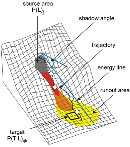
Fig. 2.Definition of rockfall hazard and related parameters (modi-fied, after Jaboyedoff et al., 2001).
– the probability that falling blocks reach a specific loca-tion on a slope (i.e. reach probability), and on
– rockfall intensity.
The latter is a complex function of block mass, velocity, ro-tation and jump height, significantly varying both along sin-gle fall paths and laterally, depending on slope morphology and rockfall dynamics (Broili, 1973; Bozzolo et al., 1988; Azzoni et al., 1995; Agliardi and Crosta, 2003; Crosta and Agliardi, 2004). Rockfall hazard can thus be better defined as the probability that a specific location on a slope is reached by a rockfall of given intensity (Jaboyedoff et al., 2001), and expressed as:
Hijk=P(L)j·P(T|L)ijk (1)
whereP(L)j is the onset probability of a rockfall event in the magnitude (e.g. volume) classj, andP(T|L)ijkis the reach probability. This is the probability that blocks trig-gered in the same event reach the locationiwith an intensity (i.e. kinetic energy) value in the classk. Since both probabil-ity and intensprobabil-ity strongly depend on the initial magnitude (i.e. mass) of rockfall events, rockfall hazard must be assessed for different magnitude scenarios, explicitly or implicitly associ-ated to different annual frequencies or return periods (Hungr et al., 1999; Dussauge-Peisser et al., 2003; Jaboyedoff et al., 2005b).
2.2 Hazard assessment
In principle, rockfall hazard assessment would require eval-uating:
a. the temporal probability (annual frequency or return pe-riod) and the spatial susceptibility of rockfall events;
b. the 3D trajectory and maximum runout of falling blocks;
c. the distribution of rockfall intensity at each location and along each fall path.
Exposed elements at risk are not considered in the def-inition of hazard. Nevertheless, hazard assessment ap-proaches should be able to deal with problems charac-terized by different spatial distributions of potentially exposed targets, point-like (houses), linear (roads, rail-ways) or areal (villages). Moreover, targets of different shape and size are likely to involve a different number of trajectories running out from different rockfall sources (Jaboyedoff et al., 2005b, Fig. 2), influencing the local reach probability. Thus, assessment methods should be able to account for the spatially distributed nature of the hazard (Crosta and Agliardi, 2003). Although several hazard assessment methods have been proposed, very few satisfy all these requirements. They differ from one another in how they account for rockfall onset frequency or susceptibility, estimated reach probability, and com-bine them to obtain quantitative or qualitative hazard ratings.
2.2.1 Onset probability and susceptibility
The frequency of events of given magnitude (volume) should be evaluated using a statistical analysis of inventories of rockfall events, taking into account the definition of suitable magnitude-frequency relationships (Dussauge-Peisser et al., 2003; Malamud et al., 2004). They are also called magni-tude - cumulative frequency distributions (MCF; Hungr et al., 1999). Although this approach is well established in the field of natural hazards (e.g. earthquakes), its application to land-slide hazards is limited by the scarce availability of data and by the intrinsic statistical properties of landslide inventories (Malamud et al., 2004). The frequency distribution of rock-fall volumes has been shown to be well fitted by the power law:
logN(V) =N0−b·logV (2)
whereN(V)is the annual frequency of rockfall with a vol-ume exceedingV,N0is the total annual frequency of
rock-fall, andbis the power law exponent, ranging between 0.4 and 0.7 (Dussauge-Peisser et al., 2003). According to Hungr et al. (1999), magnitude-cumulative frequency curves (MCF) derived from rockfall inventories allow estimating the annual frequency of rockfall events in specified volume classes, thus
Fig. 2. Definition of rockfall hazard and related parameters
(modi-fied, after Jaboyedoff et al., 2001).
Exposed elements at risk are not considered in the defini-tion of hazard. Nevertheless, hazard assessment approaches should be able to deal with problems characterised by differ-ent spatial distributions of potdiffer-entially exposed targets, point-like (houses), linear (roads, railways) or areal (villages). Moreover, targets of different shape and size are likely to in-volve a different number of trajectories running out from dif-ferent rockfall sources (Jaboyedoff et al., 2005b, Fig. 2), in-fluencing the local reach probability. Thus, assessment meth-ods should be able to account for the spatially distributed nature of the hazard (Crosta and Agliardi, 2003). Although several hazard assessment methods have been proposed, very few satisfy all these requirements. They differ from one an-other in how they account for rockfall onset frequency or sus-ceptibility, estimated reach probability, and combine them to obtain quantitative or qualitative hazard ratings.
2.2.1 Onset probability and susceptibility
of data and by the intrinsic statistical properties of landslide inventories (Malamud et al., 2004). The frequency distribu-tion of rockfall volumes has been shown to be well fitted by the power law:
logN (V )=N0−b·logV (2)
whereN (V )is the annual frequency of rockfall with a vol-ume exceedingV,N0is the total annual frequency of rock-fall andb is the power law exponent, ranging between 0.4 and 0.7 (Dussauge-Peisser et al., 2003). According to Hungr et al. (1999), magnitude-cumulative frequency curves (MCF) derived from rockfall inventories allows for the estimating of the annual frequency of rockfall events in specified vol-ume classes, thus, defining hazard scenarios. Major limita-tions to this approach include the lack of rockfall inventories for most sites and the spatial and temporal heterogeneity of available inventories. These are possibly affected by cen-soring, hampering a reliable prediction of the frequency of either very small and very large events (Hungr et al., 1999; Dussauge-Peisser et al., 2003; Malamud et al., 2004). The hazard has been completely assessed using this approach by Hungr et al. (1999) in the case of a section of highway. On a regional scale, Wieczorek et al. (1999) and Guzzetti et al. (2003) partially included the MCF within the method; while Dussauge-Peisser et al. (2002, 2003) and Vangeon et al. (2001) formalized the use of the MCF on a regional scale merging it with susceptibility mapping.
Where site-specific rockfall inventories are either unavail-able or unreliunavail-able, the analysis of rockfall hazard can only be carried out in terms of susceptibility. This is the relative probability that any slope unit is affected by rockfall occur-rence, given a set of environmental conditions (Brabb, 1984). Onset susceptibility (see Sect. 3) can be assessed
– in a spatially distributed way by heuristic ranking of se-lected instability indicators (Pierson et al., 1990; Can-celli and Crosta, 1993; Rouiller and Marro, 1997; Maz-zoccola and Sciesa, 2000; Budetta, 2004),
– by deterministic methods (Jaboyedoff et al., 2004a; Guenther et al., 2004; Derron et al., 2005) or
– by statistical methods (Frattini et al., 2008). 2.2.2 Reach probability and intensity
The reach probability and intensity for rockfall of given mag-nitude (volume) depends on the physics of rockfall processes and on topography (see Sect. 4). The simplest methods de-scribing rockfall propagation are based on the shadow
an-gle approach, according to which the maximum travel
dis-tance of blocks is defined by the intersection of the topog-raphy with an energy line having an empirically-estimated inclination (Evans and Hungr, 1993, Fig. 2). Unfortunately, with this approach there is no physical process model for rockfall and its interaction with the ground behind and only
the maximum extent of rockfall runout areas is estimated (Fig. 3a). However, this approach has been implemented in a GIS tool (CONEFALL, Jaboyedoff and Labiouse, 2003) allowing a preliminary estimation of rockfall reach suscep-tibility and kinetic energy (Fig. 3b), according to the energy
height approach (Evans and Hungr, 1993). Many existing
hazard assessment methodologies estimate reach probability and intensity using 2-D rockfall numerical modelling (Matte-rock, Rouiller and Marro,1997; Rockfall Hazard Assessment Procedure RHAP, Mazzoccola and Sciesa, 2000; Cadanav, Jaboyedoff et al., 2005b). This provides a more accurate description of rockfall physics and allows for a better eval-uation of rockfall reach probability (i.e., relative frequency of blocks reaching specific target locations) and of the spa-tial distribution of kinetic energy). However, 2-D modelling neglects the geometrical and dynamic effects of a 3-D to-pography on rockfall, leading to a subjective extension of simulation results between adjoining 2-D fall paths (Fig. 3c). Although this limitation has, in part, been overcome by intro-ducing pseudo 3-D assumptions (Jaboyedoff et al., 2005b), full 3-D numerical modelling has been shown to be required to account for the lateral dispersion of 3-D trajectories and the related effects on reach probability and intensity. Nev-ertheless, a few hazard assessment methodologies based on 3-D numerical modelling are available (Crosta and Agliardi, 2003, Fig. 3d).
2.3 Hazard zoning: current practice and unresolved questions
Rockfall hazard or susceptibility mapping/zoning is the final step of hazard assessment, leading to the drafting of a doc-ument useful for land planning, funding prioritization or the preliminary assessment of suitable protective measures. The major issue in hazard zoning is to find consistent criteria to combine onset probability or susceptibility, reach probabil-ity and intensprobabil-ity in a map document, especially when formal probabilities cannot be evaluated.
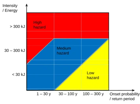
Swiss guidelines (Raetzo et al., 2002, see Fig. 4) require that rockfall hazard are zoned according to the onset proba-bility (i.e., return period) and intensity (i.e., kinetic energy), thus, defining three hazard zones, namely red, blue and yel-low. Nevertheless, these do not explicitly account for the reach probability and the spatial variability of kinetic en-ergy. Thus, Jaboyedoff et al. (2005b) proposed a method-ology (Cadanav) based on 2-D numerical modelling to map hazard according to the probability where blocks involved in events with a specified return period reach a specific location along a 2-D profile with a given kinetic energy.
A. Volkwein et al.: Review on rockfall characterisation and structural protection 2621
A. Volkwein et al.: Rockfall review 5
Fig. 3. Comparison of hazard maps derived for the area of Mt. S.Martino (Lecco, Italy; Jaboyedoff et al., 2001; Crosta and Agliardi, 2003) using different modelling approaches and zoning methods. a) Maximum runout area estimated by ashadow angle
approach using the code CONEFALL (Jaboyedoff and Labiouse, 2003); b) hazard map obtained by applying the RHV methodology (Crosta and Agliardi, 2003) to the reach probability and kinetic en-ergy estimated by CONEFALL; c) rockfall hazard map obtained by 2D numerical modelling using the RHAP methodology (modified after Mazzoccola and Sciesa, 2000); d) rockfall hazard map ob-tained by 3D numerical modelling using the code HY-STONE and the RHV methodology (modified after Crosta and Agliardi, 2003).
evaluation of onset susceptibility by means of multivariate statistical techniques.
When drafting hazard maps for practical purposes, it must be kept in mind that the reliability (and practical applicabil-ity) of hazard maps depends on a number of factors. The description of rockfall dynamics are adopted to model rock-fall trajectories (e.g. 2D or 3D, empirical, kinematical or dynamic). This way, complex phenomena such as block fragmentation or the effects of vegetation are accounted for (Crosta et al., 2004; Dorren et al., 2004) and greatly influ-ence all the hazard components related to rockfall propaga-tion, and thus the final hazard map. The spatial resolution of the adopted description of topography, especially when 3D models are used, controls primarily the lateral dispersion of rockfall trajectories and of the computed dynamic quan-tities, thus affecting the local reach probability and inten-sity (Crosta and Agliardi, 2004). The applicability of hazard models on different scales and with different aims also de-pends on model resolution, thus requiring tools with
multi-Intensity / Energy
High hazard > 300 kJ
Medium hazard 30 – 300 kJ
Low < 30 kJ
hazard < 30 kJ
Onset probability / return period 1 – 30 y 30 – 100 y 100 – 300 y
Fig. 4.Hazard classification for rockfall in Switzerland
scale assessment capabilities. Major uncertainties in rockfall hazard mapping are also related to the uncertainty of rockfall onset frequency when required (e.g. Swiss Code). This is of-ten unknown, thus requiring that a set of scenario-based haz-ard maps rather than a single map are produced (Jaboyedoff et al., 2005b). From this perspective, the choice of thedesign block volume scenario is critical to avoid eitherrisky under-estimation or cost-ineffective overunder-estimation of a hazard. Fi-nally, the extent of mapped hazard zones is greatly influenced by subjectivity in establishing class boundaries for parame-ters contributing to the hazard. These should be constrained by physically-based criteria depending on the envisaged use of the maps (e.g. land planning or countermeasure design; Crosta and Agliardi, 2003; Jaboyedoff et al., 2005b).
2.4 From hazard to quantitative risk assessment
Although hazard mapping is a useful tool for land planning, risk analysis should be carried out to support the design and optimization of both structural and non-structural protection actions (Fell et al., 2005; Straub and Schubert, 2008). Never-theless, a standard risk analysis approach for rockfall is yet to be proposed because of the still difficult assessment of haz-ards. In fact, when a hazard is expressed as susceptibility, risk can only be assessed through relative scales or matrices (Guzzetti et al., 2004; Fell et al., 2005). The simplest form of rockfall risk analysis consists of analysing the distribution of elements at risk with different postulated vulnerability in different hazard zones (Acosta et al., 2003; Guzzetti et al., 2003, 2004). However, this approach does not fully account for the probability of rockfall impact, the vulnerability and value of exposed targets. Guidelines for Quantitative Risk Analysis (QRA) based on Hong Kong rockfall inventories (Chau et al., 2003) were proposed by GEO (1998), whereas Straub and Schubert (2008) combined probability theory and 2D numerical modelling in order to improve risk analysis for
Fig. 3. Comparison of hazard maps derived for the area of Mt. S. Martino (Lecco, Italy; Jaboyedoff et al., 2001; Crosta and Agliardi, 2003) using different modelling approaches and zoning methods. (a) Maximum runout area estimated by a shadow angle approach using the code CONEFALL (Jaboyedoff and Labiouse, 2003); (b) hazard map obtained by applying the RHV methodology (Crosta and Agliardi, 2003) to the reach probability and kinetic en-ergy estimated by CONEFALL; (c) rockfall hazard map obtained by 2-D numerical modelling using the RHAP methodology (modified after Mazzoccola and Sciesa, 2000); (d) rockfall hazard map ob-tained by 3-D numerical modelling using the code HY-STONE and the RHV methodology (modified after Crosta and Agliardi, 2003).
large scale susceptibility mapping, based on the use of on-set susceptibility indicators and the shadow angle method (Fig. 3a). Mazzoccola and Sciesa (2000) proposed a method-ology (RHAP) in which 2-D numerical simulation is used to zone reach probability along profiles, later weighted ac-cording to indicators of cliff activity (Fig. 3c). Crosta and Agliardi (2003) combined reclassified values of reach sus-ceptibility and intensity values such as kinetic energy or jump height derived by distributed 3-D rockfall modelling to obtain a physically-based index (Rockfall Hazard Vector, RHV). This allows for a quantitative ranking of hazards, ac-counting for the effects of 3-D topography (Fig. 3d) while keeping information about the contributing parameters. This approach was implemented by Frattini et al. (2008) to include a quantitative evaluation of onset susceptibility by means of multivariate statistical techniques.
When drafting hazard maps for practical purposes, it must be kept in mind that the reliability (and practical
applicabil-A. Volkwein et al.: Rockfall review 5
Fig. 3. Comparison of hazard maps derived for the area of Mt. S.Martino (Lecco, Italy; Jaboyedoff et al., 2001; Crosta and Agliardi, 2003) using different modelling approaches and zoning methods. a) Maximum runout area estimated by ashadow angle
approach using the code CONEFALL (Jaboyedoff and Labiouse, 2003); b) hazard map obtained by applying the RHV methodology (Crosta and Agliardi, 2003) to the reach probability and kinetic en-ergy estimated by CONEFALL; c) rockfall hazard map obtained by 2D numerical modelling using the RHAP methodology (modified after Mazzoccola and Sciesa, 2000); d) rockfall hazard map ob-tained by 3D numerical modelling using the code HY-STONE and the RHV methodology (modified after Crosta and Agliardi, 2003).
evaluation of onset susceptibility by means of multivariate statistical techniques.
When drafting hazard maps for practical purposes, it must be kept in mind that the reliability (and practical applicabil-ity) of hazard maps depends on a number of factors. The description of rockfall dynamics are adopted to model rock-fall trajectories (e.g. 2D or 3D, empirical, kinematical or dynamic). This way, complex phenomena such as block fragmentation or the effects of vegetation are accounted for (Crosta et al., 2004; Dorren et al., 2004) and greatly influ-ence all the hazard components related to rockfall propaga-tion, and thus the final hazard map. The spatial resolution of the adopted description of topography, especially when 3D models are used, controls primarily the lateral dispersion of rockfall trajectories and of the computed dynamic quan-tities, thus affecting the local reach probability and inten-sity (Crosta and Agliardi, 2004). The applicability of hazard models on different scales and with different aims also de-pends on model resolution, thus requiring tools with
multi-Intensity / Energy
High hazard > 300 kJ
Medium hazard 30 – 300 kJ
Low < 30 kJ
hazard < 30 kJ
Onset probability / return period 1 – 30 y 30 – 100 y 100 – 300 y
Fig. 4.Hazard classification for rockfall in Switzerland
scale assessment capabilities. Major uncertainties in rockfall hazard mapping are also related to the uncertainty of rockfall onset frequency when required (e.g. Swiss Code). This is of-ten unknown, thus requiring that a set of scenario-based haz-ard maps rather than a single map are produced (Jaboyedoff et al., 2005b). From this perspective, the choice of thedesign block volume scenario is critical to avoid eitherrisky under-estimation or cost-ineffective overunder-estimation of a hazard. Fi-nally, the extent of mapped hazard zones is greatly influenced by subjectivity in establishing class boundaries for parame-ters contributing to the hazard. These should be constrained by physically-based criteria depending on the envisaged use of the maps (e.g. land planning or countermeasure design; Crosta and Agliardi, 2003; Jaboyedoff et al., 2005b).
2.4 From hazard to quantitative risk assessment
Although hazard mapping is a useful tool for land planning, risk analysis should be carried out to support the design and optimization of both structural and non-structural protection actions (Fell et al., 2005; Straub and Schubert, 2008). Never-theless, a standard risk analysis approach for rockfall is yet to be proposed because of the still difficult assessment of haz-ards. In fact, when a hazard is expressed as susceptibility, risk can only be assessed through relative scales or matrices (Guzzetti et al., 2004; Fell et al., 2005). The simplest form of rockfall risk analysis consists of analysing the distribution of elements at risk with different postulated vulnerability in different hazard zones (Acosta et al., 2003; Guzzetti et al., 2003, 2004). However, this approach does not fully account for the probability of rockfall impact, the vulnerability and value of exposed targets. Guidelines for Quantitative Risk Analysis (QRA) based on Hong Kong rockfall inventories (Chau et al., 2003) were proposed by GEO (1998), whereas Straub and Schubert (2008) combined probability theory and 2D numerical modelling in order to improve risk analysis for
Fig. 4. Hazard classification for rockfall in Switzerland
ity) of hazard maps depends on a number of factors. Dif-ferent descriptions of rockfall dynamics can be adopted to model rockfall trajectories (e.g., 2-D or 3-D, empirical, kine-matical or dynamic). Moreover, complex phenomena, such as block fragmentation or the effects of vegetation, may be accounted for in different ways (Crosta et al., 2004; Dor-ren et al., 2004) and greatly influence all the hazard com-ponents related to rockfall propagation and, thus, the final hazard map. The spatial resolution of the adopted descrip-tion of topography, especially when 3-D models are used, controls primarily the lateral dispersion of rockfall trajecto-ries and the computed dynamic quantities, thus, affecting the local reach probability and intensity (Crosta and Agliardi, 2004). The applicability of hazard models on different scales and with different aims also depends on model resolution, thus, requiring tools with multi-scale assessment capabili-ties. Major uncertainties in rockfall hazard zoning are also related to the uncertainty of rockfall onset frequency when required (e.g., Swiss Code). This is often unknown, thus, re-quiring that a set of scenario-based hazard maps rather than a single map are produced (Jaboyedoff et al., 2005b). From this perspective, the choice of the design block volume sce-nario is critical to avoid either risky underestimation or cost-ineffective overestimation of a hazard. Finally, the extent of mapped hazard zones is greatly influenced by subjectivity in establishing class boundaries for parameters contributing to the hazard. These should be constrained by physically-based criteria depending on the envisaged use of the maps (e.g. land planning or countermeasure design; Crosta and Agliardi, 2003; Jaboyedoff et al., 2005b).
actions (Fell et al., 2005; Straub and Schubert, 2008). Never-theless, a standard risk analysis approach for rockfall is yet to be proposed because of the still difficult assessment of haz-ards. In fact, when a hazard is expressed as susceptibility, risk can only be assessed through relative scales or matrices (Guzzetti et al., 2004; Fell et al., 2005). The simplest form of rockfall risk analysis consists of analysing the distribution of elements at risk with different postulated vulnerability in different hazard zones (Acosta et al., 2003; Guzzetti et al., 2003, 2004). However, this approach does not fully account for the probability of rockfall impact, the vulnerability and value of exposed targets. Guidelines for Quantitative Risk Analysis (QRA) based on Hong Kong rockfall inventories (Chau et al., 2003) were proposed by GEO (1998), whereas Straub and Schubert (2008) combined probability theory and 2-D numerical modelling in order to improve risk analysis for single countermeasure structural design. Bunce et al. (1997) and Hungr et al. (1999) quantitatively estimated rockfall risk along highways in British Columbia, based on inventories of rockfall events. Nevertheless, major efforts are still re-quired to perform a quantitative evaluation of rockfall risk in spatially distributed situations (e.g., urban areas; Corominas et al., 2005), where long runout and complex interactions be-tween rockfall and single elements at risk occur, requiring a quantitative assessment of vulnerability.
In this perspective, Agliardi et al. (2009) proposed a quan-titative risk assessment framework exploiting the advantages of 3-D numerical modelling to integrate the evaluation of the temporal probability of rockfall occurrence, the spatial prob-ability and intensity of impacts on structures, their vulnera-bility, and the related expected costs for different protection scenarios. In order to obtain vulnerability curves based on physical models for reinforced concrete buildings, Mavrouli and Corominas (2010) proposed the use of Finite Element (FE)-based progressive collapse modelling.
3 Rockfall source areas 3.1 Influencing factors
As pointed out in Sect. 2, the rockfall hazardH at a given location and for a given intensity and scenario depends on two terms, namely: the onset probability (i.e., temporal fre-quency of rockfall occurrence) of a rockfall instability event and the probability of propagation to a given location (see Eq. 1) (Jaboyedoff et al., 2001). The latter,P (T|L)ij k, can be evaluated by propagation modelling or by observation. In order to evaluateP (L), it is first necessary to identify poten-tial rockfall sources, whereas their susceptibility is mainly based on rock slope stability analysis or estimates and can be evaluated by field observations or modelling. Anyway, it must be kept in mind that inventories are the only direct way to derive the true hazard in small areas. For rockfall involving limited volumes (i.e., fragmental rockfall, usually
<100 000 m3) methods of rock slope stability analysis are well established and their application is relatively easy when the slope and the source area are well characterised (Hoek and Bray, 1981; Norrish and Wyllie, 1996; Wyllie and Mah, 2004). However, this procedure does not give any informa-tion about time-dependence and is difficult to apply on a re-gional scale (Guenther et al., 2004).
Most rockfall source area assessment methods are based on stability assessment or on rockfall activity quantification. In order to get an estimate of rockfall activity, either inven-tories or indirect methods, such as dendrochronology, are needed (Perret et al., 2006; Corominas et al., 2005). Several parameters can be used to create a hazard map for rockfall source areas, which, most of the time, involves susceptibility mapping (Guzzetti et al., 1999). The parameters used de-pend mainly on the availability of existing documents or the budget available to collect field information (Jaboyedoff and Derron, 2005).
Source area susceptibility analysis has often used multi-parameter rating systems derived from tunnelling and mining engineering, such as Rock Mass Rating (Bieniawski, 1973, 1993, RMR;). Its evolution to the Slope Mass Rating SMR (Romana, 1988, 1993) led to more suitable results by adding an explicit dependence on the joint-slope orientation rela-tionship. Recently, Hoek (1994) introduced the Geological Strength Index (GSI) as a simplified rating of rock quality. In recent years, it has been applied successfully to slope sta-bility analysis (Brideau et al., 2007). A similar approach was proposed by Selby (1980, 1982) for geomorphological appli-cations. Later, with the increasing availability of digital ele-vation models (DEM; Wentworth et al., 1987; Wagner et al., 1988) and of geographic information systems (GIS), several other techniques (heuristic and probabilistic) have been ex-plored (Van Westen, 2004). However, this can be refined con-ceptually because a slope system can be described in terms of internal parameters (IP) and external factors (EF), which pro-vide a conceptual framework to describe the instability po-tential using the available data (Fig. 5). Therefore, instability detection requires locating (1) the pre-failure processes and (2) the areas sensitive to rapid strength degradation leading to slope failure (Jaboyedoff et al., 2005a; Leroueil and Locat, 1998). IP are the intrinsic features of the slopes. Some exam-ples are summarized below (Jaboyedoff and Derron, 2005):
(a) Morphology: slope types (slope angle, height of slope, profile, etc.), exposure, type of relief (depends on the controlling erosive processes), etc.
(b) Geology: rock types and weathering, variability of the geological structure, bedding, type of deposit, folded zone, etc.
(c) Fracturing: joint sets, trace lengths, spacing, fracturing intensity, etc.
A. Volkwein et al.: Review on rockfall characterisation and structural protection 2623
6 A. Volkwein et al.: Rockfall review
single countermeasure structural design. Bunce et al. (1997) and Hungr et al. (1999) quantitatively estimated rockfall risk along highways in British Columbia, based on inventories of rockfall events. Nevertheless, major efforts are still re-quired to perform a quantitative evaluation of rockfall risk in spatially distributed situations (e.g. urban areas; Corominas et al., 2005), where long runout and complex interactions be-tween rockfall and single elements at risk occur, requiring a quantitative assessment of vulnerability.
Thus, Agliardi et al. (2009) proposed a quantitative risk assessment framework exploiting the advantages of 3D nu-merical modelling to integrate the evaluation of the temporal probability of rockfall occurrence, the spatial probability and intensity of impacts on structures, their vulnerability, and the related expected costs for different protection scenarios. In order to obtain vulnerability curves based on physical mod-els for reinforced concrete buildings, Mavrouli and Coromi-nas (2010) proposed the use of Finite Element (FE)-based progressive collapse modelling.
3 Rockfall source areas
3.1 Influencing factors
As pointed out in Section 2, the rockfall hazardHat a given location and for a given intensity and scenario depends on two terms, namely: the onset probability (i.e. temporal fre-quency of rockfall occurrence) of a rockfall instability event and the probability of propagation to a given location (see Eq. 1) (Jaboyedoff et al., 2001). The latter,P(T|L)ijk, can
be evaluated by propagation modelling or by observation. In order to evaluateP(L)it is first necessary to identify po-tential rockfall sources whereas their susceptibility is mainly based on rock slope stability analysis or estimates and can be evaluated by field observations or modelling. Anyway, it must be kept in mind that inventories are the only direct way to derive thetrue hazard in small areas. For rockfall involving limited volumes (i.e. fragmental rockfall, usually
<100,000m3) methods of rock slope stability analysis are
well established and their application is relatively easy when the slope and the source area are well characterized (Hoek and Bray, 1981; Norrish and Wyllie, 1996; Wyllie and Mah, 2004). However, this procedure does not give any informa-tion about time-dependence and is difficult to apply on a re-gional scale (Guenther et al., 2004).
Most rockfall source area assessment methods are based on stability assessment or on rockfall activity quantification. In order to get an estimate of rockfall activity either in-ventories or indirect methods such as dendrochronology are needed (Perret et al., 2006; Corominas et al., 2005). Several parameters can be used to create ahazardmap for rockfall source areas, which, most of the time, involves susceptibility mapping (Guzzetti et al., 1999). The parameters used de-pend mainly on the availability of existing documents or the
Fig. 5.EF and IP for rockfall (modified from Jaboyedoff and Labi-ouse, 2003; Jaboyedoff and Derron, 2005).
budget available to collect field information (Jaboyedoff and Derron, 2005).
Source area susceptibility analysis has often used multi-parameter rating systems derived from tunnelling and mining engineering, such as Rock Mass Rating (Bieniawski, 1973, 1993, RMR;). Its evolution to the Slope Mass Rating SMR (Romana, 1988, 1993) led to more suitable results by adding an explicit dependence on the joint-slope orientation rela-tionship. Recently, Hoek (1994) introduced the Geological Strength Index (GSI) as a simplified rating of rock quality. In recent years, it has been applied successfully to slope sta-bility analysis (Brideau et al., 2007). A similar approach was proposed by Selby (1980, 1982) for geomorphological appli-cations. Later, with the increasing availability of digital ele-vation models (DEM; Wentworth et al., 1987; Wagner et al., 1988) and of geographic information systems (GIS) several other techniques (heuristic and probabilistic) have been ex-plored (Van Westen, 2004). However, this can be refined con-ceptually because a slope system can be described in terms of internal parameters (IP) and external factors (EF), which pro-vide a conceptual framework to describe the instability po-tential using the available data (Fig. 5). Therefore, instability detection requires locating (1) the pre-failure processes and (2) the areas sensitive to rapid strength degradation leading to slope failure (Jaboyedoff et al., 2005a; Leroueil and Locat, 1998). IP are the intrinsic features of the slopes. Some exam-ples are summarized below (Jaboyedoff and Derron, 2005):
a. Morphology: slope types (slope angle, height of slope, profile, etc.), exposure, type of relief (depends on the controlling erosive processes), etc.
b. Geology: rock types and weathering, variability of the geological structure, bedding, type of deposit, folded zone, etc.
c. Fracturing: joint sets, trace lengths, spacing, fracturing intensity, etc.
Fig. 5. EF and IP for rockfall (modified from Jaboyedoff and
Labi-ouse, 2003; Jaboyedoff and Derron, 2005).
(e) Activity: movements or rockfall, etc.
(f) Hydrogeology: permeability, joint permeability, etc. Note that within a given framework, the joint sets or discon-tinuities are the anisotropies that mainly control the stability (Hoek and Bray, 1981); points b to d are related to these properties. The link between rockfall activity and the inten-sity of pre-existing fracturing, as in fold hinges with a steep limb, has been demonstrated by Coe and Harp (2007).
The IP can evolve with time due to the effects of the EF, which are (Jaboyedoff and Derron, 2005):
– gravitational effects;
– water circulation: hydrology or hydrogeology, climate, precipitation in the form of rainfall or snow, infiltration rates, groundwater;
– weathering; – erosion; – seismicity; – active tectonics;
– microclimate including freezing and thawing, sun ex-posure, permafrost, which are increasingly invoked to explain rockfall activities (Frayssines, 2005; Matsuoka and Sakai, 1999; Matsuoka, 2008; Gruner, 2008); – nearby instabilities;
– human activities (anthropogenic factors); – etc.
These lists of internal parameters and external factors are not exhaustive, but allow one to introduce key points for the
following different methods that have been proposed to as-sess the value of failure frequencyP (L)in general by using susceptibility mapping. GIS and related software allow one to manage most of these parameters regionally. For example, in Switzerland the 1:250000 topographic vectorized maps include the cliff area as polygons (Jaboyedoff and Labiouse, 2003; Loye et al., 2009).
3.2 Methods of identification and description 3.2.1 Methods using regional geomechanical
approaches
Basically, methods such as the Rock Fall Hazard Rating Sys-tem (RFHRS, Pierson et al., 1990) or the Missouri Rockfall Hazard Rating System (MRFHRS, Maerz et al., 2005) mix bothP (L)andP (T |L)estimates at the same level, as well as risk. Both methods are designed for talus slopes close to roads and have been refined in two ways, i.e., simplifying the number of parameters from 12 (or 18) to 4 for the RHRS (Santi et al., 2008) or by mixing them with the RMS param-eters (Budetta, 2004). These methods mix IP and EF at the same levels.
In addition to the classical rock mass characterisation (Bi-eniawski, 1973; Romana, 1988), some methods are proposed to regionalise susceptibility parameters. Using mixed IP and EF Mazzoccola and Hudson (1996) developed a rating sys-tem based on the matrix interaction approach of the Rock En-gineering System (RES) methodology (Hudson, 1992). This allows one to create a modular rock mass characterisation method of slope susceptibility ranking. Based on a similar approach, Vangeon et al. (2001) proposed to calibrate a sus-ceptibility scale using a geotechnical rating with a regional inventory, designed for a linear cliff area (Carere et al., 2001). Rouiller et al. (1998) developed a susceptibility rating system based on 7 criteria mixing IP and EF.
3.2.2 GIS and DEM analysis-based methods
with the scree slopes. This can be performed either using the shadow angle method (Baillifard, 2005) or the HY STONE programme by intersecting the trajectory simulation with the scree slopes (Frattini et al., 2008).
Along one particular road in Switzerland, five parame-ters: proximity to faults, nearness of a scree slope, cliff height, steep slope and proximity to road, were used to obtain good results using a simple classical GIS approach (Bailli-fard et al., 2003).
The major improvement related to GIS or/and the use of DEM is the automatic kinematical analysis (Wagner et al., 1988; Rouiller et al., 1998; Gokceoglu et al., 2000; Dorren et al., 2004; G¨unther, 2003; Guenther et al., 2004), which al-lows one to determine whether the discontinuity sets are able to create instabilities. Using the standard stability criterion (Norrish and Wyllie, 1996) and a statistical analysis of the kinematical tests, Gokceoglu et al. (2000) were able to pro-duce maps of probability of sliding, toppling or wedge type failures. G¨unther (2003) and Guenther et al. (2004) used a partial stability analysis using a Mohr-Coulomb criterion and an estimate of the stress state at a given depth of about 20 m at each pixel of the DEM, also integrating in the analysis the regionalisation of discontinuities such as folded bedding and geology. The number of slope failures linked to joint sets depends on the apparent discontinuity density at the ground surface, which can also be used as an input for the rock slope hazard assessment and to identify the most probable failure zone (Jaboyedoff et al., 2004b). In addition to structural tests, it may also be possible to combine several of the EF and IP, such as water flow, erodible material volume, etc., to obtain a rating index (Baillifard et al., 2004; Oppikofer et al., 2007). Rock failure is mainly controlled by discontinuities. The main joint sets can be extracted from the orientation of the to-pography (DEM) using different methods and software (Der-ron et al., 2005; Jaboyedoff et al., 2007; Kemeny et al., 2006; Voyat et al., 2006). Extracting the discontinuity sets from DEM allows one to perform a kinematic test on a regional area (Oppikofer et al., 2007). New techniques such as ground based LiDAR DEM allow one to extract the full structures, even in the case of inaccessible rock cliffs (Lato et al., 2009; Sturzenegger et al., 2007a; Voyat et al., 2006).
In landslide hazard assessment, many statistical or other modern techniques are now used (Van Westen, 2004); e.g., Aksoy and Ercanoglu (2006) classified the susceptibility of source areas using a fuzzy logic-based evaluation. 3.3 Concluding remarks on source detection
Until now, most rock slope systems have been described by considering the EFs and IPs that control stability. This pro-cedure only gives approximate results, mainly because field access is usually limited. Moreover, to assess the hazard from susceptibility maps remains very difficult. Neverthe-less, recently developed technologies like photogrammetry or LiDAR (Kemeny et al., 2006) permit one to extract high
quality data from DEM that – regarding some points – is bet-ter than that from standard fieldwork, especially for geologi-cal structures (joint sets, fractures). However, for a logeologi-cal fully detailed analysis, on-site inspection using Alpine techniques is unavoidable in order to correctly asses the amount of open-ings, fillings or roughness of joints or to verify automatically determined rock face properties.
At the present time, the attempt to extract information such as GSI from LiDAR DEM is still utopian (Sturzenegger et al., 2007b), but we can expect future generations of terrestrial Li-DAR to allow the extraction of such information. The anal-ysis of geological structures in high resolution DEM and the simulation of all possible instabilities in a slope have already been performed at the outcrop level (Grenon and Hadjigeor-giou, 2008). We can expect that such methods will be ap-plicable on a regional scale within the next 10 yr by using remote-sensing techniques associated with limited field ac-quisition that will provide rock parameters, structures and include stability simulations. However, the goal of hazard assessment will not be reached as long as this analysis does not account for temporal dependencies. That can only be achieved if we understand the failure mechanisms, i.e., the degradation of the IP under the action of EF, such as weath-ering (Jaboyedoff et al., 2007). Expected climate changes will affect the frequency and magnitude of the EF. There is a need to understand their impact on rock slope stability, other-wise we will either miss or overestimate a significant amount of potential rockfall activity.
4 Trajectory modelling
It is important to describe the movement of a falling rock along a slope, i.e., its trajectory. This allows the description of existing hazard susceptibility or hazard assessment for a certain area. In addition, the information on boulder velocity, jump heights and spatial distribution is the basis for correct design and the verification of protective measures.
A description of rockfall trajectories can be roughly ob-tained by analytical methods (see Sect. 4.4.1). If more de-tailed analyses are needed and stochastic information has to be considered, numerical approaches are recommended.
A. Volkwein et al.: Review on rockfall characterisation and structural protection 2625 4.1 Types of rockfall model
4.1.1 2-D rockfall trajectory models
We define a 2-D trajectory model as a model that simulates the rockfall trajectory in a spatial domain defined by two axes. This can be a model that calculates along a user-defined slope profile (Azzoni et al., 1995) that is defined by a dis-tance axis (x or y) and an altitude axis (z). Such a profile often follows the line of the steepest descent. Table 1 shows that the majority of the rockfall trajectory models belongs to this group. In the second type of 2-D model rockfall tra-jectories are calculated in a spatial domain defined by two distance axes x and y, e.g., a raster with elevation values or a map with contour lines. Such models generally calculate the rockfall path using topographic-hydrologic approaches and velocity and runout distance with a sliding block approach (cf. Van Dijke and van Westen, 1990; Meissl, 1998). As such these models do not provide information on rebound heights. 4.1.2 2.5-D rockfall trajectory models
The second group of trajectory models defined here are 2.5-D models, also called quasi-3-2.5-D models. These are simply 2-D models assisted by GIS to derive pre-defined fall paths. The key characteristic of such models is that the direction of the rockfall trajectory in the x,y domain is independent of the kinematics of the falling rock and its trajectory in the vertical plane. In fact, in these models the calculation of the
hori-zontal fall direction (in the x,y domain) could be separated
completely from the calculation of the rockfall kinematics and the rebound positions and heights. This means that these models actually carry out two separate 2-D calculations. The first one determines the position of a slope profile in an x,y domain and the second one is a 2-D rockfall simulation along the previously defined slope profile. Examples of such mod-els are those that calculate rockfall kinematics along a slope profile that follows the steepest descent as defined using dig-ital terrain data, as in the model Rocky3 (Dorren and Seij-monsbergen, 2003).
4.1.3 3-D rockfall trajectory models
These models are defined as trajectory models that calcu-late the rockfall trajectory in a 3-dimensional plane (x, y, z) during each calculation step. As such, there is an in-terdependence between the direction of the rockfall trajec-tory in the x,y domain, the kinematics of the falling rock, its rebound positions and heights and if included, impacts on trees. Examples of such models are EBOUL-LMR (De-scoeudres and Zimmermann, 1987), STONE (Guzzetti et al., 2002), Rotomap (Scioldo, 2006), DDA (Yang et al., 2004), STAR3-D (Dimnet, 2002), HY-STONE (Crosta et al., 2004) and Rockyfor3-D (Dorren et al., 2004), RAMMS:Rockfall (Christen et al., 2007); Rockfall-Analyst (Lan et al., 2007), PICUS-ROCKnROLL (Rammer et al., 2007; Woltjer et al.,
2008) or as shown in Masuya et al. (1999). The major advan-tage of 3-D models is that diverging and converging effects of the topography, as well as exceptional or surprising trajecto-ries, i.e., those that are less expected at first sight in the field, are clearly reflected in the resulting maps. A disadvantage of 3-D models is the need for spatially explicit parameter maps, which require much more time in the field than parameter value determination for slope profile-based trajectory simu-lations.
4.2 Calculation approaches
A second main characteristic that allows one to distinguish between different rockfall trajectory models, which is closely related to the calculation of the rebound, is the representation of the simulated rock in the model. As shown in Table 1, this can be done firstly by means of a lumped mass, i.e., the rock is represented by a single, dimensionless point. The second approach is the rigid body, i.e., the rock is represented by a real geometrical shape, which is often a sphere, cube, cylin-der or ellipsoid. In general, this approach is used in the deter-ministic models mentioned above. The last approach is the hybrid approach, i.e., a lumped mass approach for simulat-ing free fall and a rigid body approach for simulatsimulat-ing rollsimulat-ing, impact and rebound (Crosta et al., 2004; Frattini et al., 2008; Agliardi et al., 2009).
Most of the rockfall trajectory models use a normal and a tangential coefficient of restitution for calculating the re-bound of simulated rock on the slope surface and a fric-tion coefficient for rolling. Details on these coefficients are, among others, presented in Guzzetti et al. (2002). An overview of typical values of the coefficients of restitu-tion can be found in Scioldo (2006). The models that use these coefficients generally apply a probabilistic approach for choosing the parameter values used for the actual re-bound calculation (see Table 1). This is to account for the large variability in the real values of these parameters, due to the terrain, the rock shape and the kinematics of the rock during the rebound. Bourrier et al. (2009b) pre-sented a new rebound model that linked the impact angle, the translational and the rotational velocity before and after the rebound based on multidimensional, stochastic functions, which gave promising results for rocky slopes. There are also models that use deterministic approaches for calculat-ing the rockfall rebound. These models use mostly a discrete element method (Cundall, 1971), such as the Discontinuous Deformation Analysis (Yang et al., 2004) or percussion the-ory (Dimnet, 2002).
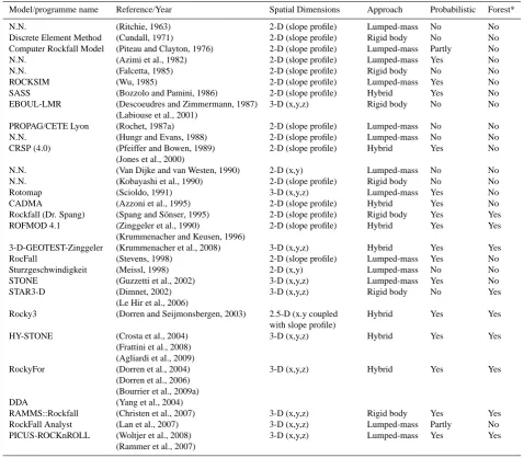
Table 1. Main characteristics of a selection of existing rockfall trajectory models (modified from Guzzetti et al., 2002).
Model/programme name Reference/Year Spatial Dimensions Approach Probabilistic Forest*
N.N. (Ritchie, 1963) 2-D (slope profile) Lumped-mass No No
Discrete Element Method (Cundall, 1971) 2-D (slope profile) Rigid body No No
Computer Rockfall Model (Piteau and Clayton, 1976) 2-D (slope profile) Lumped-mass Partly No
N.N. (Azimi et al., 1982) 2-D (slope profile) Lumped-mass Yes No
N.N. (Falcetta, 1985) 2-D (slope profile) Rigid body No No
ROCKSIM (Wu, 1985) 2-D (slope profile) Lumped-mass Yes No
SASS (Bozzolo and Pamini, 1986) 2-D (slope profile) Hybrid Yes No
EBOUL-LMR (Descoeudres and Zimmermann, 1987) 3-D (x,y,z) Rigid body No No
(Labiouse et al., 2001)
PROPAG/CETE Lyon (Rochet, 1987a) 2-D (slope profile) Lumped-mass No No
N.N. (Hungr and Evans, 1988) 2-D (slope profile) Lumped-mass No No
CRSP (4.0) (Pfeiffer and Bowen, 1989) 2-D (slope profile) Hybrid Yes No
(Jones et al., 2000)
N.N. (Van Dijke and van Westen, 1990) 2-D (x,y) Lumped-mass No No
N.N. (Kobayashi et al., 1990) 2-D (slope profile) Rigid body No No
Rotomap (Scioldo, 1991) 3-D (x,y,z) Lumped-mass Yes No
CADMA (Azzoni et al., 1995) 2-D (slope profile) Hybrid Yes No
Rockfall (Dr. Spang) (Spang and S¨onser, 1995) 2-D (slope profile) Rigid body Yes Yes
ROFMOD 4.1 (Zinggeler et al., 1990) 2-D (slope profile) Hybrid Yes Yes
(Krummenacher and Keusen, 1996)
3-D-GEOTEST-Zinggeler (Krummenacher et al., 2008) 3-D (x,y,z) Hybrid Yes Yes
RocFall (Stevens, 1998) 2-D (slope profile) Lumped-mass Yes No
Sturzgeschwindigkeit (Meissl, 1998) 2-D (x,y) Lumped-mass No No
STONE (Guzzetti et al., 2002) 3-D (x,y,z) Lumped-mass Yes No
STAR3-D (Dimnet, 2002) 3-D (x,y,z) Rigid body No Yes
(Le Hir et al., 2006)
Rocky3 (Dorren and Seijmonsbergen, 2003) 2.5-D (x.y coupled with slope profile)
Hybrid Yes Yes
HY-STONE (Crosta et al., 2004) 3-D (x,y,z) Hybrid Yes Yes
(Frattini et al., 2008) (Agliardi et al., 2009)
RockyFor (Dorren et al., 2004) 3-D (x,y,z) Hybrid Yes Yes
(Dorren et al., 2006) (Bourrier et al., 2009a)
DDA (Yang et al., 2004)
RAMMS::Rockfall (Christen et al., 2007) 3-D (x,y,z) Rigid body Yes Yes
RockFall Analyst (Lan et al., 2007) 3-D (x,y,z) Lumped-mass Partly No
PICUS-ROCKnROLL (Woltjer et al., 2008) 3-D (x,y,z) Lumped-mass Yes Yes
(Rammer et al., 2007)
∗Forest characteristics such as tree density and corresponding diameters can be taken into account explicitly
4.3 Block-slope interaction
The trajectories of falling rocks can be described as com-binations of four types of motion: free fall, rolling, sliding and bouncing of a falling block (Ritchie, 1963; Lied, 1977; Descoeudres, 1997). The occurrence of each of these types strongly depends on the slope angle (Ritchie, 1963). For steep slopes, free fall is most commonly observed, whereas for intermediate slopes, rockfall propagation is a succession of free falls and rebounds. For gentle slopes, the prevalent motion types are rolling or sliding.
A significant number of rockfall simulation programmes exist to perform trajectory analyses. The challenge is not in the free flight simulation, but in modelling the interactions
A. Volkwein et al.: Review on rockfall characterisation and structural protectionA. Volkwein et al.: Rockfall review 262711
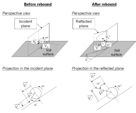
Fig. 6.Definition of the block velocity before and after rebound.
Vn+components of the velocity after rebound also allow the
definition of a plane called the reflected plane. The angleδ
between these two planes is called the deviation angle. The normal, tangential and rotationalω+velocities after rebound
are computed from the normal, tangential and rotationalω−
velocities before rebound using a rebound model, and the deviation angleδis determined, leading to the complete def-inition of the rock velocity after rebound.
4.3.1 Sliding and rolling models
Sliding mainly occurs at small velocities, when a block starts to move or comes to rest. It is not accounted for in many rockfall models because it does not entail large propagations of the blocks. Pure rolling is quite a rare motion mode, except on soft soils when the boulder penetrates the soil (Bozzolo and Pamini, 1986; Ritchie, 1963). The distinction between the rolling and sliding modes is sometimes difficult since a combination of the two movements can occur (Descoeudres, 1997; Giani, 1992). On stiffer outcropping materials, due to the slope surface’s irregularity and the rock shape, the rolling motion is more a succession of small bounces.
Therefore, most rockfall models simulate trajectories as successions of free fall and bouncing phases. Only a few con-sider sliding and rolling motions (e.g., Azzoni et al., 1995; Bozzolo and Pamini, 1986; Statham, 1979). In these models a tangential damping coefficient related to the rolling and/or sliding friction between block and slope is introduced. The sliding friction is defined by means of the normal compo-nent with respect to the soil surface of the block’s weight ac-cording to Coulomb’s law. For rolling motion, acac-cording to Statham (1979), a fairly accurate description is also given by using Coulomb’s law with a rolling friction coefficient that depends on the characteristics of the block (size and shape)
and the slope (type and size of debris).
The transition condition between the bouncing and the rolling mode is discussed in Piteau (1977), Hungr and Evans (1988) and Giani (1992). The transition from sliding to rolling is defined in Bozzolo et al. (1988).
The whole rockfall trajectory is sometimes modelled as the sliding or rolling of a mass on a sloping surface with an aver-age friction angle assumed to be representative of the mean energy losses along the block’s path (Evans and Hungr, 1993; Govi, 1977; Hungr and Evans, 1988; Japan Road Associa-tion, 1983; Lied, 1977; Rapp, 1960; Toppe, 1987b). This method (called the Fahrb¨oschung, the shadow angle or the cone method) provides a quick and low-cost preliminary de-lineation of areas endangered by rockfall, either on a local or a regional scale (Jaboyedoff and Labiouse, 2003; Meissl, 2001).
4.3.2 Rebound models
Bouncing occurs when the falling block collides with the slope surface. The height of the bounce and the rebound di-rection depend on several parameters characterizing the im-pact conditions. Of the four types of movement that occur during rockfall, the bouncing phenomenon is the least well understood and the most difficult to predict.
A number of rockfall models represent the rebound in a simplified way by one or two overall coefficients, which are called restitution coefficients. Some models use only one restitution coefficient, quantifying the dissipation in terms of either velocity magnitude loss (Kamijo et al., 2000; Paronuzzi, 1989; Spang and Rautenstrauch, 1988; Spang and S¨onser, 1995) or kinetic energy loss (e.g., Azzoni et al., 1995; Bozzolo and Pamini, 1986; Chau et al., 1999a; Ur-ciuoli, 1988). In this case, an assumption regarding the re-bound direction is necessary to fully determine the velocity vector after impact (i.e. theα+angle in Figure 6). TheRv
coefficient is considered for the formulation in terms of ve-locity loss and the RE coefficient is used for the formula-tion in terms of kinetic energy (neglecting in general the ro-tational part):
RV = V
+
V− and RE=
1/2[I(ω+)2+m(V+)2]
1/2[I(ω−)2+m(V−)2] (3)
However, the most common definition of block rebound involves differentiation into tangential Rt and normal Rn
restitution coefficients (Budetta and Santo, 1994; Evans and Hungr, 1993; Fornaro et al., 1990; Giani, 1992; Guzzetti et al., 2002; Hoek, 1987; Kobayashi et al., 1990; Pfeiffer and Bowen, 1989; Piteau and Clayton, 1976; Urciuoli, 1988; Ushiro et al., 2000; Wu, 1985):
Rt = Vt+
Vt− and Rn= V+
n Vn−
(4)
These coefficients are used conjointly and characterize the decrease in the tangential and the normal components of the
Fig. 6. Definition of the block velocity before and after rebound.
There are other programmes that could be considered as hybrid, taking advantage of the fast and easy simulation of free flight for lumped masses while considering geometri-cal and mechanigeometri-cal characteristics of the slope and the block to model the impact (Azimi and Desvarreux, 1977; Bozzolo and Pamini, 1986; Dorren et al., 2004; Jones et al., 2000; Kobayashi et al., 1990; Pfeiffer and Bowen, 1989; Rochet, 1987b; Crosta et al., 2004).
If 3-D rockfall simulations are based on a “pseudo-2-D” approach (see Sect. 4) the block’s tangential Vt− and nor-malVn− velocity components (before rebound) with respect to the slope surface allow definition of a plane called the inci-dent plane (Fig. 6). Similarly, the tangentialVt+and normal Vn+components of the velocity after rebound also allow the definition of a plane called the reflected plane. The angleδ between these two planes is called the deviation angle. The normal, tangential and rotationalω+velocities after rebound are computed from the normal, tangential and rotationalω− velocities before rebound using a rebound model, and the deviation angleδis determined, leading to the complete def-inition of the rock velocity after rebound.
4.3.1 Sliding and rolling models
Sliding mainly occurs at small velocities, when a block starts to move or comes to rest. It is not accounted for in many rockfall models because it does not entail large propagations of the blocks. Pure rolling is quite a rare motion mode, except on soft soils when the boulder penetrates the soil (Bozzolo and Pamini, 1986; Ritchie, 1963). The distinction between the rolling and sliding modes is sometimes difficult since a combination of the two movements can occur (Descoeudres, 1997; Giani, 1992). On stiffer outcropping materials, due to
the slope surface’s irregularity and the rock shape, the rolling motion is more a succession of small bounces.
Therefore, most rockfall models simulate trajectories as successions of free fall and bouncing phases. Only a few con-sider sliding and rolling motions (e.g., Azzoni et al., 1995; Bozzolo and Pamini, 1986; Statham, 1979). In these models a tangential damping coefficient related to the rolling and/or sliding friction between block and slope is introduced. The sliding friction is defined by means of the normal compo-nent with respect to the soil surface of the block’s weight ac-cording to Coulomb’s law. For rolling motion, acac-cording to Statham (1979), a fairly accurate description is also given by using Coulomb’s law with a rolling friction coefficient that depends on the characteristics of the block (size and shape) and the slope (type and size of debris).
The transition condition between the bouncing and the rolling mode is discussed in Piteau and Clayton (1977), Hungr and Evans (1988) and Giani (1992). The transition from sliding to rolling is defined in Bozzolo et al. (1988).
The whole rockfall trajectory is sometimes modelled as the sliding or rolling of a mass on a sloping surface with an aver-age friction angle assumed to be representative of the mean energy losses along the block’s path (Evans and Hungr, 1993; Govi, 1977; Hungr and Evans, 1988; Japan Road Associa-tion, 1983; Lied, 1977; Rapp, 1960; Toppe, 1987b). This method (called the Fahrb¨oschung, the shadow angle or the cone method) provides a quick and low-cost preliminary de-lineation of areas endangered by rockfall, either on a local or a regional scale (Jaboyedoff and Labiouse, 2003; Meissl, 2001).
4.3.2 Rebound models
Bouncing occurs when the falling block collides with the slope surface. The height of the bounce and the rebound di-rection depend on several parameters characterising the im-pact conditions. Of the four types of movement that occur during rockfall, the bouncing phenomenon is the least under-stood and the most difficult to predict.
A number of rockfall models represent the rebound in a simplified way by one or two overall coefficients, which are called restitution coefficients. Some models use only one restitution coefficient, quantifying the dissipation in terms of either velocity magnitude loss (Kamijo et al., 2000; Paronuzzi, 1989; Spang and Rautenstrauch, 1988; Spang and S¨onser, 1995) or kinetic energy loss (e.g., Azzoni et al., 1995; Bozzolo and Pamini, 1986; Chau et al., 1999a; Ur-ciuoli, 1988). In this case, an assumption regarding the re-bound direction is necessary to fully determine the veloc-ity vector after impact (i.e., the α+ angle in Fig. 6). The Rv coefficient is considered for the formulation in terms of velocity loss and theRE coefficient is used for the formu-lation in terms of kinetic energy (neglecting in general the rotational part):
RV =
V+
V− and RE=
1/2[I (ω+)2+m(V+)2]