Window Flow Control in Stochastic Network Calculus - The General Service Case

Window Flow Control in Stochastic Network Calculus –

The General Service Case

Michael Beck

Distributed Computer Systems Lab (DISCO) Germany

[email protected]

Jens Schmitt

Distributed Computer Systems Lab (DISCO) Germany

[email protected]

ABSTRACT

The problem of Window Flow Controlled (WFC) systems has been analysed successfully in Deterministic Network Cal-culus (DNC). While many results of DNC have been carried over to its stochastic extension, the problem of WFC sys-tems has not been solved so far. This paper presents the first approach to analyse WFC in the context of Stochas-tic Network Calculus (SNC) for a general service inside the feedback loop of the controller. The key idea is to keep track of how much the service deviates from being subaddi-tive. The new method is illustrated in numerical examples and its properties are discussed.

Categories and Subject Descriptors

C.4 [Computer Systems Organization]: Performance of Systems—Modeling techniques

General Terms

Theory

Keywords

Stochastic Network Calculus, Feedback, Flow Control

1.

INTRODUCTION

Stochastic Network Calculus (SNC) has matured in recent years to provide an alternative method for performance anal-ysis of stochastic queueing systems (see e.g. [15, 13, 9]). Many results from the deterministic network calculus (DNC) have been transferred into the stochastic domain, some have been rather immediate some have required considerable ef-fort (e.g., deriving the end-to-end service [7]). One major remaining open issue is the stochastic analysis of feedback-based systems, such as Window Flow Controlled (WFC) transport protocols, e.g. TCP. While there are very ele-gant solutions for WFC in the deterministic setting [1, 5, 16], WFC in SNC has been identified for some time already as a very challenging open research question [15, 12, 13, 8]. Moreover, being able to analyse WFC systems in SNC would

be very relevant to open up new application areas for SNC such as modelling smart grid systems [14], for instance.

In this paper, we present an approach to analyse WFC in SNC under very general assumptions. As we demonstrate below, as long as the service in the feedback loop is subad-ditive the analysis is a rather direct transfer from DNC (see [3] for a detailed discussion, where especially the continu-ous time case needs care, though). Yet, the assumption of a subadditive service inside the feedback loop is restrictive and there are several scenarios where subadditivity cannot be assumed; most prominently, this is the case if a tandem of servers has to be traversed. This is why we tackle the hard case of general service in the feedback loop in this work.

The key idea of our approach is to stochastically control how far the service deviates from being subadditive and cast this into the setting of MGF-calculus [6, 11], a branch of SNC, as further contribution to the violation probabilities of the performance bounds. We demonstrate the method by providing some numerical results in case of a server in the feedback loop that is not subadditive and would thus not be analysable by direct methods (compare [3]).

2.

NOTATION AND SOME BASIC RESULTS

First, we provide the notation and some basic results of (de-terministic) network calculus. For further details one can also refer to [4, 6]. For ease of presentation we assume a discrete time model throughout this work, see [3] for results on continuous time.

We start by defining (arrival) flows, which represent a fluid stream of data. These flows enter and depart service ele-ments.

Definition 1. We denote an arrival flowby its cumula-tives A; i.e., A(t) units of data arrive in the interval [0, t]. The bivariate extension of Ais defined by:

A(s, t) :=A(t)−A(s).

Note that flows are always additive, i.e.

A(s, t) =A(s, r) +A(r, t)

for allr, s, t.

We introduce two service descriptions here, one for the

uni-VALUETOOLS 2015, December 14-16, Berlin, Germany Copyright © 2016 ICST

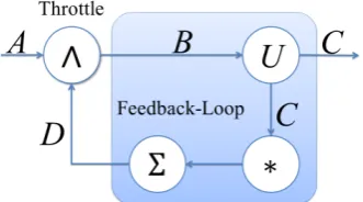
Figure 1: A window flow controller: the inputA is throttled at the ∧-element. The departures of the system are C and the feedback-loop consists of the dynamic U-server, an unspecified service element and a window-element. The star is a placeholder for zero, one, or more elements, like delay elements, scalers or dynamic servers.

variate calculus (usually used in DNC and the tail-bound-branch of SNC) and the bivariate calculus (used in the MGF-branch of SNC):

Definition 2. We say a service element offers aservice

curveU, if for any input-output pairA, B and timet

B(t)≥A⊗U(t) := min

0≤s≤t{A(s) +U(t−s)}.

LetU be a bivariate function with U(s, t)≤U(s, t0) for all

t≤t0. We say a service element is a dynamicU-server, if for any input-output pairA, B and time t:

B(t)≥A⊗U(0, t) := min

0≤s≤t{A(0, s) +U(s, t)}.

The operators ⊗ are called (univariate or bivariate) min-plus convolution, as they resemble the ordinary convolution operator under standard algebra. Note that the bivariateU

is in general not additive, i.e., there may exist r, s, t with

U(s, t)6=U(s, r) +U(r, t). The serviceU can, however, be

subadditive, i.e., for allr, s, t:

U(t)≤U(s) +U(t−s) (1)

U(s, t)≤U(s, r) +U(r, t) (2)

in the univariate and bivariate case, respectively.

The following is crucial for the end-to-end analysis of net-works consisting of several service elements.

Theorem 3. Consider two service elements, such that the output of the first service element is the input to the second. If both service elements have a service curveUi(are a dynamicUi-server,i= 1,2), the system also has a service curve, given byU1⊗U2 (is a dynamicU1⊗U2-server).

The second network-operation we give here is central to this work. It describes how a WFC system as presented in Figure 1 is handled. In this feedback system, the original inputAis fed to a throttle-element first, which governs how much data is admitted to the inside of the system (the feedback-loop).

This is realized by taking the minimum of the inputAand the output of the service element at any time, such that:

B(t) =A(t)∧D(t).

Such systems are studied for example in [1, 5, 16, 6]. We formulate from there the following theorem:

Theorem 4. Assume the whole feedback-loop in

Figure 1 is described by a service curveUf b (is a dynamic

Uf b-server). The throttle element∧has a service curveU∧

(is a dynamicU∧-server), with:

U∧(t) = ∞

^

k=0

U_{f b}(k)(t), U∧(s, t) = ∞

^

k=0

U_{f b}(k)(s, t) !

.

Here the notationU_{f b}(k)stands for thek-fold self-convolution ofUf b. Further, for anyU we defineU(0) to be the neutral

element of the convolution: U(0)(t) =1(t) =∞for allt >0 and 1(0) = 0 (for the bivariate case we have 1(s, t) = ∞ for alls < tand1(t, t) = 0 for allt, respectively). The ex-pressionV∞

k=0U (k)

=:U is known as thesubadditive closure

of service U. As the name suggests the subadditive closure of a service description is subadditive. Further, we have for any subadditiveU:

∞

^

k=0

U(k)=1∧U.

To complete the analysis of the feedback system in Figure 1 we apply Theorem 4 and Theorem 3 and get a service description for the whole system by:

Usys=U∧⊗U.

This service description can then be used to derive perfor-mance bounds, like end-to-end-delay, as detailed later.

In network calculus one typically assumes systems to be empty at time zero, i.e., for all participating flows holds

A(0) = 0. The window element in the feedback-loop serves two purposes: 1) it kick-starts our system, by initially ad-mitting a certain amount of data toUand 2) it controls how much data is present inside the feedback-loop, thus guaran-teeing a maximum backlog, which may occur on any element inside of it.

Definition 5. A window element Σ is a function from

N0 to R+0, such that for any input-flow A it produces an

outputB

B(t) =A(t) + Σ(t) (3)

Σ(s, t)≥ −A(s, t) ∀s≤t. (4)

We further define the bivariatesΣ(s, t)as for flows.

is not a flow: we do not have the property that Σ(t)≤Σ(t0) for allt≤t0.

One can rewrite the properties of a window element in the form of service curves (if Σ is constant) or dynamic servers (for time-varying window sizes):

B(t) =A⊗WΣ(0, t)

with

WΣ(t) =

(

Σ ift= 0 ∞ else

or

WΣ(s, t) =

(

Σ(t) ifs=t

∞ ifs < t

Note, however, as Σ is missing monotonicity, it is not a service curve (dynamic server) in the sense of Definition 2.

Using the above calculus one can derive probabilistic per-formance bounds. To this end we define two perper-formance measures of a system with input-output pairA,B:

Definition 6. The backlog q of the system at time tis defined by:

q(t) :=A(t)−B(t).

The virtual delaydat timetis defined by:

d(t) := min{T : A(t)≤B(t+T)}.

So far we have expressed the theory of network calculus in terms of its flows and service processes. To calculate stochas-tic bounds onq anddwe need to add a probabilistic com-ponent on top of that. There are different methods [13] to describe the stochastic nature of flows and service descrip-tions each leading to their own slightly different performance guarantees. The one we use in this paper is provided in the following theorem [6, 11]:

Theorem 7. Let time be discrete and let the arrival flow

A and the service process U be stochastically independent. Letθ >0, such that there exist bounds:

E(eθA(s,t))≤eθρA(θ)(t−s)+θσA(θ) (5) E(e−θU(s,t))≤eθρU(θ)(t−s)+θσU(θ) (6)

for alls≤tandρA(θ) +ρU(θ) =:ρ(θ)<0. Then:

P(q(t)> x)≤eθ(σA(θ)+σU(θ)−x)(1−eθρ(θ))−1 ∀t≥0

P(d(t)> T)≤eθ(σA(θ)+σU(θ)+ρU(θ)T)(1−eθρ(θ))−1 ∀t≥0.

The conditionρ(θ)<0 is a stability condition for the sys-tem. There are versions of the above theorem for contin-uous time, as well as for the case in which A and U are not stochastically independent [2]. The above bounds use Moment-Generating Functions (MGFs) to describe the be-haviour ofAandU, which is why it is called MGF-calculus for short.

We point out here that none of the state-of-the-art methods is able to describe the service process resulting from Theo-rem 4 efficiently. This is why the solution of WFC systems eluded stochastic network calculus, so far.

3.

PROBLEM EXPOSITION

Subadditivity plays an important role when analysing WFC systems, as the throttle’s service is just the subadditive closure of the elements inside the feedback loop. Hence, feedback-loops containing subadditive elements are much easier to analyse. We present this situation now in detail.

We look at a feedback loop which contains a subadditive service elementU (lying on the path from the sender to the receiver) and a window-element (lying on the return path). Such a system can be easily analysed, by applying the most general result concerning WFC systems as found in the text-book of Chang [6]. To that end, denote the space of bivari-ate functions which are monotonically increasing in their second variable as ˜F. We see immediately that all flows and all dynamic-server descriptions lie in ˜F, as they fulfill

F(s, t)≤F(s, t0) for allt≤t0.

Definition 8. An operator π : F˜ → F˜ is called σ-additiveif:

π

∞

^

n=1 Fn

!

=

∞

^

n=1

π(Fn), (7)

whereFnis any sequence inF˜and the infima are understood pointwisely.

One can easily verify that the space ofσ-additive operators is closed under taking countable minima and compositions. Further they distribute over countable minima:

∞

^

n=1 πn

!

◦π=

∞

^

n=1

(πn◦π), π◦

∞

^

n=1 πn

!

=

∞

^

n=1

(π◦πn)

An example of aσ-additive operator is the convolution with some bivariateU ∈F, defined by˜ πU(A) :=A⊗U. Other

examples needed for our specific feedback system are

π˜e(A) :=A

π+w(A)(s, t) :=

(

A(s, t) ifs6= 0

A(0, t) +w ifs= 0

where w ∈ R. The above operators represent the

iden-tity operator and a window-element, respectively; their σ -additivity as well as the following properties are easy to ver-ify:

• π+w commutes withπU, i.e. πU◦π+w=π+w◦πU.

• π2

+w=π+2w, andU is subadditive withU(t, t) = 0 for

alltiffπU is idempotent, i.e. πU2 =πU.

itself:

πf b:=π+w◦πU,

i.e. D = πf b(B). The relations between the flows in

Figure 1 are hence given by:

B(t) =A(t)∧πf b(B)(0, t). (8)

Lemma 5.7.2. in [6] can be applied resulting inB≥πf b?(A)

for any B fulfilling B ≥ A ∧ πf b(B), where

π?f b=πe˜∧V∞_n=1πnf bis the closure ofπf b.

We show now thatπ?

f b is tractable when considering a

sub-additiveU together with a window-element.

Example 9. Applying the above properties toπf b, we ob-serve that

πnf b≥π+nw◦πU.

And for the closure ofπf b

π?f b≥πe˜∧

∞

^

n=1

π+nw◦πU=π˜e∧πU.

Applying the result of Chang we have for the departures C

of the feedback system:

C(t)≥πU(B)(0, t)≥πU◦πf b? (A)(0, t)

=

∞

^

n=0

πU◦πf bn(A)(0, t)

≥

∞

^

n=0

π+nw◦πU(A)(0, t) =πU(A)(0, t)

We use the distributivity ofσ-additive operators in the sec-ond line. We see that the whole system behaves, just like the unthrottled one. With given MGF-bounds on A and U we can use this bound onC to produce stochastic performance bounds, as in Theorem 7.

The above example makes the role of subadditivity clear: withoutU being subadditive, we would not have π2

U =πU

and the description ofπ?

f b would includeπUn. The repeated

application ofπU prevents deriving stochastic performance

bounds as above. Note further, that the window-element causes only minor difficulties, as its operator commutes with

πU.

The most important example for a non-subadditiveU is a service, which results from applying Theorem 3. How one can preserve subadditivity instead for a concatenation of service elements is discussed in [3]. However, preserving subadditivity in that way comes at the cost of a decreased service.

We now leave the notations of σ-additive operators, and take a step back to have a closer look at subadditivity in the most simple scenario. For this discussion we retreat to the univariate case and let the placeholder in Figure (1) be empty. Further, we assume a window-element of fixed size, such thatUf b=U+ Σ.

As the subadditive closure of the feedback-loop appears in the solution of Theorem 4, subadditivity of the service curve

U and how much is “missing” to it are crucial questions in WFC systems. Assume we can give the following bound, describing by what quantity a service curveU fails subaddi-tivity:

U(t)−U⊗U(t)≤b ∀t∈R+0. (9)

Or, written differently:

U(2)(t)≥U(t)−b ∀t∈R+0.

If we consider some U and b to fulfill Equation (9), we achieve for Σ≥bthe subadditivity ofU+ Σ =Uf b, since

(U+ Σ)⊗(U+ Σ)(t) =U(2)(t) + 2Σ ≥U(t)−b+ 2Σ ≥U(t) + Σ =Uf b(t).

A subadditiveUf b, however means that1

Usys(t) =Uf b⊗U(t) = (1∧U+ Σ)⊗U(t) =U(t).

This effect, that a system with a large enough window can be analysed as unthrottled, is well known and can for example be found in [1]. One can think of the window-element to compensate for how the service deviates from subadditivity.

4.

WFC WITH GENERAL SERVICE

We revisit the solution of Theorem 4. Without further as-sumptions, we need to find an MGF-bound in the sense of (6) for the end-to-end service:

Usys=

∞

^

n=0

(Uf b)(n)

!

⊗U(s, t),

whereUf brepresents the whole feedback-loop. Just applying

the definition of the MGF we obtain

ΦUsys(s,t)(−θ)

=E(e−θ

V

(Uf b)(n)⊗U(s,t)_{) =} E(

∞

_

n=0 e−θU

(n)

f b ⊗U(s,t)_).

A naive approach would be to useE(X∨Y)≤E(X) +E(Y)

for some positive random variablesX andY, resulting in:

ΦUsys(s,t)(−θ)≤

∞

X

n=0 E(e−θU

(n)

f b ⊗U(s,t)₎

This however is problematic, since finite representations, as in (6) forU_{f b}(n)withn→ ∞, are hard to achieve, even ifUf b

consists of a single serverU and the window element Σ only.

Remembering condition (9) we choose another path here. To fix notations, insert for the placeholder in Figure (1) a dynamicV-server, such thatUf b(s, t) =U⊗V(s, t) + Σ(t).

We saw in the univariate case for b <Σ an easy solution to the feedback inequality. The same holds for the bivariate setting with a dynamic window; assume it holds for alls≤t:

U⊗V(s, t)−(U⊗V)(2)(s, t)≤b≤Σmin(t) (10)

1

with Σmin(t) := mins≤t{Σ(s)}. Then we have:

Uf b⊗Uf b(s, t)

= min

s≤r≤t{U⊗V(s, r) + Σ(r) +U⊗V(r, t) + Σ(t)}

≥ min

s≤r≤t{U⊗V(s, r) +U⊗V(r, t)}+ Σmin(t) + Σ(t)

≥U⊗V(s, t) + (Σmin(t)−b) + Σ(t)

≥Uf b(s, t)

andUf b is subadditive.

We use this property to achieve a service description for the whole system by:

Usys(s, t)

=Uf b⊗U(s, t) = (1∧Uf b)⊗U(s, t) (11)

=U(s, t)∧ min

s≤r≤t{(U⊗V)(s, r) + Σ(r) +U(r, t)}

≥U(s, t)∧(U⊗V)⊗(U⊗V)(s, t) + Σmin(t) (12)

(10)

≥ U(s, t)∧U⊗V(s, t)−b+ Σmin(t)

≥U(s, t)∧U⊗V(s, t) (13) =U⊗V(s, t).

In (12) and we used the monotonicty of min-plus convolu-tion:U(s, t)≥U⊗V(s, t) for anyV withV(t, t) = 0 for all

t. So, under the assumption of (10) we obtain at least the same service for the throttled system as for an unthrottled one where the serversU andV would have to be traversed. Hence, we are interested in the probability of (10) happen-ing and call that eventE. With this information at hand we can analyse the whole system by:

P(dsys(t)> x)

=P(dsys(t)> x|E)P(E) +P(dsys(t)> x| ¬E)P(¬E) (14)

≤P(dU⊗V(t)> x) +P(¬E)

where P(dU⊗V > x) can be calculated by applying

Theorem 3 and Theorem 7.

We now discuss condition (10) and its corresponding prob-ability. For ease of presentation, we leave the placeholder blank, i.e.,U⊗V =U.

One can rewrite (10) by:

max

0≤s≤t{U(s, t)−U⊗U(s, t)} ≤b,

which is just the expression we arrive at when bounding the buffer in bivariate deterministic network calculus, if feeding a “flow”U in a dynamicU ⊗U-server. Such stochastically dependent systems can be analysed in MGF-Calculus by using H¨older’s inequality. For this assume some MGF-bounds of the form (5) and (6) forU (we denote theσandρ corre-sponding to bound (5) byσandρto distinguish them from the ones used in (6)). The probabilistic backlog bound in

such a system is (1

p+

1

q =

1

p0 +_q10 = 1):

P(q(t)> b)≤P( max

0≤s≤t{U(s, t)−U⊗U(s, t)}> b)

≤e−θb

t

X

s=0

E(eθ(U(s,t)−U⊗U(s,t)))

≤e−θb

t

X

s=0

(E(epθU(s,t)))1/p(E(e−θqU⊗U(s,t)))1/q

≤e−θb

t

X

s=0

eθρ¯(pθ)(t−s)+θσ¯(pθ)(E(e−θqU⊗U(s,t)))1/q

≤e−θb+θσ¯(pθ)

t

X

s=0

eθρ¯(pθ)(t−s)

·

t

X

r=s

eθqρ(qp0θ)(r−s)+θqσ(qp0θ)eθqρ(qq0θ)(t−r)+θqσ(qq0θ)

1/q

≤e−θb+θσ¯(pθ)+θσ(qp0θ)+θσ(qq0θ)

·

t

X

s=0

eθρ¯(pθ)(t−s)eθρ(qp0θ)(t−s)

t−s

X

r0₌₀

eθq(ρ(qq0θ)−ρ(qp0θ))r0

1/q

We have used Chernoff’s inequality in the second line and H¨older’s inequality in line 3 and 5. If we assume, w.l.o.g. thatq0 > p0 holds, we have that the last sum is convergent int. We denote the limit of that series just byB and can proceed with:

P(q(t)> b)

≤e−θb+θ(¯σ(pθ)+σ(qp0θ)+σ(qq0θ))B

t

X

s=0

eθρ¯(pθ)(t−s)+θρ(qp0θ)(t−s)

≤e−θb+θ(¯σ(pθ)+σ(qp0θ)+σ(qq0θ))B

t

X

s0₌₀

eθ( ¯ρ(pθ)+θρ(qp0θ))s0.

The above sum, however, does in general not converge. This is due to the three inequalities:

¯

ρ(pθ)≥ρ¯(θ) ∀p≥1,

¯

ρ(θ)≥ −ρ(θ) ∀θ≥0,

−ρ(θ)≥ −ρ(qθ) ∀q≥1.

For the case q0 = p0 = 2, the exponents in the last sum vanish and the expression reduces to t−s+ 1 ≤eθ(t−s)1θ_,

such that the bound becomes:

P(q(t)> b)

≤e−θb+θ(¯σ(pθ)+2σ(2qθ))

t

X

s0₌₀

eθ( ¯ρ(pθ)+θρ(2qθ)+qθ1)s

0

.

Note that the system −U→U →U is unstable (the concate-nation of the two servers with serviceU ⊗U is at most as large as the arrivals U), which is why the above bound is valid only for any finite timet.

Overall, we can summarize our findings in the main result of this paper:

Let 1

p+

1

q =

1

p0 +_q10 = 1andq

0

> p0. Assume the following MGF-bounds onU⊗V:

E(e−θU⊗V(s,t))≤eθρ(θ)(t−s)+σ(θ) E(eθU⊗V(s,t))≤eθρ(θ)(t−s)+σ(θ).

The whole system fulfills the probabilistic delay-bound:

P(dsys(t)> x)≤P(dU⊗V(t)> x)

+e−θΣmin(t+T)+σE(θ,p,p0)_B

t+T

X

s=0

eθρE(θ,p,p0)s

with

σE(θ, p, p0) =σ(pθ) +σ(qp0θ) +σ(qq0θ)

ρE(θ, p, p

0

) = (

ρ(pθ) +ρ(qp0θ) ifp06= 2

ρ(pθ) +ρ(2qθ) +_qθ1 ifp0= 2

B= 





1

1−eθq(ρ(qq0θ)−ρ(qp0θ) 1/q

ifp06= 2

1 ifp0= 2

anddU⊗V being the delay of an unthrottled tandem consist-ing of a dynamicU- andV-server.

We want to emphasize that with this theorem it is for first time possible to analyse a general WFC system in the con-text of SNC. Our solution does not rely on the subadditivity ofU or V directly, in contrast to what was presented in Section 3 and [3]. Instead we ask for the prob-ability of failing the subadditivity by at least the window size Σ, which allows an analysis of general service elements inside the feedback loop. Note thatU and V do not need to be single service elements themselves, they could instead result from Theorem 3 or include further elements (like fixed delay-elements or scaling elements [10]).

Remark 11. It is interesting to note, that, ifU ⊗V is

subadditive already, we haveP(¬E) = 0 and the whole

sys-tem’s service reduces immediately to

Usys(s, t) =U(s, t)∧U⊗V(s, t) + Σmin(t).

One can directly apply Theorem 7 onUsysto achieve an end-to-end delay bound in this case. Further, we observe that step (13) is not a necessary one. We could, for example, shiftbbelowΣmin(t)and continue directly with:

Usys(s, t)≥U(s, t)∧U⊗V(s, t) + Σmin(t)−b. (15)

We can then apply Theorem 10 on this Usys (which is at least as large asU⊗V). One can view this as a shift in the violation probabilities towards the subadditive part (eventE) of the bound. We investigate this tradeoff in the following section.

5.

NUMERICAL EVALUATION

In this section, we investigate how the bound derived in The-orem 10 evolves in its parameters. Further, we quantify the impact of WFC on the delay of the system, by comparing it to a similar unthrottled system. For this section we assume

U to be a constant rate server Uo(s, t) = u(t−s), which

also serves a crossflow AU(s, t) at higher priority than B.

A well-known result in SNC states that B receives a ser-viceU(s, t) =u(t−s)−AU(s, t). Similarly, we insert for the

placeholder in Figure 1 a service elementV, which also offers a constant rateVo(s, t) =v(t−s) shared with a higher

prior-ity crossflowAV(s, t), such thatV(s, t) =v(t−s)−AV(s, t).

Note that both service descriptions are subadditive by them-selves, but when applying Theorem 3 this property is lost.

To account for the typically smaller size of acknowledge-ments flowing back to the throttle, we assume v > u. The crossflows in this example consist of i.i.d. exponentially dis-tributed increments aU(t) andaV(t), respectively. The

ar-rivals to the WFC system, denoted byAalso consist of i.i.d. exponentially distributed increments. All flows are stochas-tically independent of each other. More sophisticated cross-flows or arrivals are possible to analyse, as well as dropping the independency assumption, yet this is not the focus of our evaluation. We further assume a constant window-size Σ, for all timest≥0.

A corresponding unthrottled system would just consist of the flow A being fed into the service element U, thus Theorem 7 could be applied directly.

To achieve reasonable values in the bounds of Theorem 7 and Theorem 10, we numerically optimized the parameterθ

and the H¨older-pairsp, q, p0, q0. If not specified otherwise we used the following set of parameters in our calculations: the bound is taken at timet= 5 and asks for a delayT = 10, i.e., we consider the probabilityP(dsys(5)>10). The parameter

of the exponential distributions for the arrivals and cross-flows is given by λ= 4 (we assume all three flows to have the same rate λ for simplicity), while the server-rates are

u= 1 andv= 2. This corresponds to a utilization of 50% and 25%, respectively. We present the results for a window size of Σ = 15.

5.1

Throttled vs. Unthrottled System

First we want to compare the system to its unthrottled coun-terpart. To that end, we alter the arrival ratesλ, resulting in utilizations from 30% to 80%. We plot the corresponding violation probabilities for the performance bounds on a loga-rithmic scale for the throttled, as well as the unthrottled sys-tem. We did this for different window-sizes Σ = 10,15,20. The results are displayed in Figure 2 as black and blue lines for the throttled and unthrottled system, respectively. As expected, the throttled system behaves better, the larger Σ is; for Σ = 20 the throttled system behaves almost identi-cally to the unthrottled one.

5.2

Dependence on Delay

A major difference between the unthrottled and the throt-tled analysis lies in the dependency on the delayT. While for the unthrottled system an increase inTleads to a decrease in the violation probability, we see in the bound of Theorem 10, that the term P(¬E) increases in T. In

Figure 3, one sees for the black line how the bound evolves for an increasingT. The two red lines show how the bound differs when choosingb=Σ₂, 9Σ₁₀ as suggested in Remark 11 (Equation (15)). The trend here for larger T is, that the bound becomes worse, the larger the difference between b

0.3 0.4 0.5 0.6 0.7 0.8

1e

−

16

1e

−

12

1e

−

08

1e

−

04

1e+00

Utilization in %

Violation Prob

.

Sigma = 10 Sigma = 15 Sigma = 20

Figure 2: A graph showing the violation probabili-ties depending on the utilization of throttled (black) and unthrottled (blue) systems for different window sizes. The red lines are equal to1,10−3 _{and 10}−6_.

0 5 10 15 20 25 30

1e

−

05

1e

−

04

1e

−

03

1e

−

02

1e

−

01

Delay T

Violation Prob

.

b = 0.5 Sigma b = 0.9 Sigma

Figure 3: A graph showing how the bound evolves when increasing the delayT. The red colored lines represent a shift towards the violation probability of eventE.

scenario, trading a higher violation probability for the event

E is not worthwhile the gain from a better service descrip-tionUsys.

To investigate the composition of the delay bound further, we separated the two parts of the bound in Figure 4. The blue circles correspond to the delay-part of the violation probabilityP(dU⊗V(t)> x) and the red circles correspond

to the violation probability of eventE, while the solid black circles are the sum of both. It can be clearly observed that from a certain point onwards the probabilityP(¬E)

domi-nates the overall violation probability. The additional lines drawn into the graph show how the different parts of the bound are affected when we use b = Σ₂, 3Σ₄ , 9Σ₁₀ in Equa-tion (15). It can be seen that the delay-part (blue) of the probability experiences no considerable change, while the probability of violating eventE(red) increases significantly, whenb <Σ.

2 4 6 8 10 12 14

1e

−

10

1e

−

07

1e

−

04

1e

−

01

Delay T

Violation Prob

.

b = 0.5 Sigma b = 0.75 Sigma b = 0.9 Sigma

Figure 4: A graph showing the different components of the violation probability: the blue circles are the delay-part, while the red circles represent the subadditivity-part. The black circles are the sum of both parts. The lines show the same for different shifts towards the violation probabilityP(¬E).

5.3

Convergence to Unthrottled System

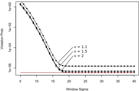
In Figure 5, we consider the convergence of the throttled sys-tem towards the unthrottled one when increasing the win-dow size. Clearly, from Theorem 10 the violation probability

P(¬E) vanishes for increasing window sizes. However, the

throttled system does not fully converge to the unthrottled one, since the delay-part of the bound still differs:

P(dU(t)> T)≤P(dU⊗V(t)> T).

The size of the gap, which cannot be closed by increasing the window size further is completely dependent on the service descriptions U and V. We present in the graph the same system as before, but vary v = 2,1.5,1.1. One can see clearly how the gap to the delay of the unthrottled system (red) increases, when reducing the rate ofv.

6.

CONCLUSION AND OUTLOOK

In this paper, we have dealt with the long-standing prob-lem of analysing WFC systems in SNC. While such feedback loops had been solved in deterministic network calculus more than a decade ago, its counterpart in the stochastic setting has been a well-known open problem [15, 12, 13, 8]. We presented how far subadditive service carries DNC solutions for WFC systems into stochastic network calculus (see also [3]). In that discussion, we encountered the very general notion ofσ-additive operators and saw as a tractable exam-ple a feedback-loop containing a single subadditive server. Unfortunately, this method reaches the end of the road as soon as operators appear which no longer commute, or are not idempotent. This is not untypical in applications, for example if tandems of servers are involved.

5 10 15 20 25 30 35 40

1e

−

06

1e

−

04

1e

−

02

1e+00

Window Sigma

Violation Prob

.

v = 1.1 v = 1.5 v = 2

Figure 5: A graph showing the convergence of the throttled system towards the unthrottled one, when increasing the windowΣ. The red line is the bound for the unthrottled system. The black lines show the throttled system, for different rates ofv.

analysis of WFC systems in MGF-based network calculus. The resulting bounds consist of two parts: first, a delay-bound of a conventional unthrottled system, containing the feedback loop as service; second, a probability of violating the subadditivity, by more than the window size. The struc-ture of our result makes a direct comparison between throt-tled and unthrotthrot-tled systems possible.

The analysis of WFC systems in stochastic network calcu-lus is not completed yet, but has rather just begun. While the now available methods can handle varying window sizes Σ, they can take only limited advantage of their variations. The presented method uses a backlog bound for the system

U

−→U⊗U →. The “arrivals” and “service” in this scenario are strongly correlated. While using H¨older’s inequality deals correctly with that dependence, it also neglects its possible advantages. As the arrivals and the service in this system are positively correlated one can hope to improve the bounds significantly, when taking the dependencies into account.

Besides improving bounds in the above sense, one can extend and build upon this work: one direction is to break the “end-to-end” feedback-loop into several hops, resulting in a tan-dem of WFC systems. Another interesting question would be how to effectively handle stochastic dependencies between the “upstream”-serviceU, the “down-stream”-elements and the window-process Σ. Answering this will push the applica-bility of SNC even further. By better grasping the occuring dependencies one can eventually aim at analysing systems like the window-controlled TCP in SNC.

7.

REFERENCES

[1] R. Agrawal, R. L. Cruz, C. Okino, and R. Rajan. Performance bounds for flow control protocols.

IEEE/ACM Transactions on Networking, 7(3):310–323, June 1999.

[2] M. A. Beck. A first course in stochastic network calculus. Online lecture notes, October 2013. http://goo.gl/qSIIwr.

[3] M. A. Beck and J. Schmitt. Window flow control in stochastic network calculus. Technical Report 391/15, University of Kaiserslautern, September 2015. http://goo.gl/K4sWhQ.

[4] J.-Y. Le Boudec and P. Thiran.Network Calculus - A Theory of Deterministic Queuing Systems for the Internet. Springer, 2001.

[5] C.-S. Chang. On deterministic traffic regulation and service guarantees: A systematic approach by filtering.

IEEE Transactions on Information Theory, 44(3):1097–1110, May 1998.

[6] C.-S. Chang.Performance Guarantees in Communication Networks. Springer, 2000.

[7] F. Ciucu, A. Burchard, and J. Liebeherr. A network service curve approach for the stochastic analysis of networks. InProc. of ACM SIGMETRICS, June 2005. [8] F. Ciucu, M. Fidler, J. Liebeherr, and J. Schmitt.

Network calculus.Dagstuhl Reports, pages 63–83, March 2015.

[9] F. Ciucu and J. Schmitt. Perspectives on network calculus – no free lunch, but still good value. InProc. of ACM SIGCOMM, August 2012.

[10] F. Ciucu, J. Schmitt, and H. Wang. On expressing networks with flow transformations in

convolution-form. InProc. of IEEE INFOCOM, April 2011.

[11] M. Fidler. An end-to-end probabilistic network calculus with moment generating functions. InProc. of IWQoS, June 2006.

[12] M. Fidler. Survey of deterministic and stochastic service curve models in the network calculus.IEEE Communications Surveys Tutorials, 12(1):59–86, 2010. [13] M. Fidler and A. Rizk. A guide to the stochastic

network calculus.IEEE Communications Surveys and Tutorials, 17(1):92–105, 2015.

[14] Y. Ghiassi-Farrokhfal, S. Keshav, and C. Rosenberg. Toward a realistic performance analysis of storage systems in smart grids.IEEE Transactions on Smart Grid, 6(1):402–410, Jan 2015.

[15] Y. Jiang and Y. Liu.Stochastic Network Calculus. Springer, 2008.