Reactive Data Handling
Selections by Manuel Bernhardt
Manning Author Picks
Copyright 2016 Manning Publications
www.manning.com. The publisher offers discounts on these books when ordered in quantity.
For more information, please contact
Special Sales Department Manning Publications Co. 20 Baldwin Road
PO Box 761
Shelter Island, NY 11964 Email: [email protected]
©2016 by Manning Publications Co. All rights reserved.
No part of this publication may be reproduced, stored in a retrieval system, or transmitted, in any form or by means electronic, mechanical, photocopying, or otherwise, without prior written permission of the publisher.
Many of the designations used by manufacturers and sellers to distinguish their products are claimed as trademarks. Where those designations appear in the book, and Manning
Publications was aware of a trademark claim, the designations have been printed in initial caps or all caps.
Recognizing the importance of preserving what has been written, it is Manning’s policy to have the books we publish printed on acid-free paper, and we exert our best efforts to that end. Recognizing also our responsibility to conserve the resources of our planet, Manning books are printed on paper that is at least 15 percent recycled and processed without the use of elemental chlorine.
Manning Publications Co. 20 Baldwin Road Technical PO Box 761
Shelter Island, NY 11964
Cover designer: Leslie Haimes
ISBN 9781617294198
iii
contents
Introduction iv
A
NALYZING
STREAMING
DATA
1
Analyzing streaming data
Chapter 4 from
Streaming Data
2
F
AULT
TOLERANCE
AND
RECOVERY
PATTERNS
22
Fault tolerance and recovery patterns
Chapter 12 from
Reactive Design Patterns
23
Y
OUR
FIRST
REACTIVE
WEB
APPLICATION
46
Your first reactive web application
Chapter 2 from
Reactive Web Applications
47
G
ETTING
SMART
WITH
ML
LIB
72
Getting smart with MLlib
Chapter 7 from
Spark in Action
73
M
ANAGING
DATACENTER
RESOURCES
WITH
M
ESOS
112
Managing datacenter resources with Mesos
Chapter 2 from
Mesos in Action
113
iv
Introduction
Web applications play an increasingly important role in all facets of our lives. We depend on our applications to be always available and to provide us with up-to-the-second data. This shift toward real-time data processing is also a key aspect of the Internet of Things, which the Gartner Group predicts by 2020 will include 26 billion actively-connected physical devices sending, receiving, and processing streams. That’s a lot of data.
The reactive application architecture is an answer to the requirements of high availability and resource efficiency. To provide these benefits for real-time data pro-cessing, reactive applications:
need to handle high and varying loads so they remain responsive to users;
can scale in and out, depending on demand, to make use of more or less hard-ware resources;
are built with supervision and recovery mechanisms in place to manage and recover from failure;
rely on asynchronous message-passing as a primary means of communication.
Reactive applications need to ensure that these core principles are applied across the entire stack, from resource management of servers in datacenters up to communica-tion with a user’s browser or native applicacommunica-tion.
O
ne core principle of reactive web applications is considering data as a dynamic stream rather than as a static reservoir. The following chapter intro-duces how to analyze streaming data. It covers the distributed stream-processing architecture as well as a few of the common frameworks available. It should give you an understanding of the high-level architecture and the common concerns of distributed data-streaming systems.2
Chapter 4 from
Streaming Data
by Andrew G. Psaltis
Analyzing
streaming data
In the previous chapter we spent time understanding and thinking through the importance of the message queueing tier. Remember that tier is designed to gather data from the collection tier and make it available to be moved through the rest of the streaming architecture. At this point the data is ready and waiting for us to consume and do magic with. In this chapter you’re going to learn about the analysis tier. Our goal is to develop an understanding of the underlying principles of this tier, and then in the next chapter we’ll dive into the different ways to use this tier to perform magic on the data. With that frame of reference in mind, con-sult our navigational aid in figure 4.1 to make sure you’re oriented with respect to the flow of data.
This chapter covers
In-flight data analysis
The common stream-processing architecture
3 Understanding in-flight data analysis
One thing that you may notice in figure 4.1 is that unlike in the previous chapter where we discussed the input and output of the data, in this chapter we’re only going to concern ourselves with the input. The reason for this is simple: our goal is to under-stand the core underpinnings of this tier, and in the next chapter we’ll discuss the ways we can work with the data in this tier. Therefore, we’ll hold off on talking about where the data goes from this tier until next chapter. After finishing this chapter you’ll have an understanding of the core concepts found in all the modern tools used for this tier and be ready to learn how to perform various operations on the data. All right, grab a quick coffee refill, and let’s get going.
4.1
Understanding in-flight data analysis
A key to understanding the features we’ll discuss in this chapter is first coming to grips with what in-flight data means and the concept of continuous queries. If the term in-flight makes you think of something that’s in the air moving and not touching the ground, that’s the right idea. When it comes to data, in-flight refers to all the tuples in
the system from the input source (the message queueing tier) to the output to a client (the next tier), the idea being that the data is always in motion and never at rest, meaning that it’s never persisted to durable storage. If you haven’t heard of the term
data at rest, don’t worry; it’s just a fancy way of saying that the data is stored on disk or another storage medium. Take a look at figure 4.2, which shows how this plays out in our streaming architecture.
Looking at figure 4.2, it should be clear that our goal in this tier is to pull the data from the message queueing tier as fast as possible; ideally the analysis tier should be able to keep up with the rate at which the collection tier is pushing data into the mes-sage queueing tier. So how is this different from a non-streaming system, say one built with a traditional DBMS (RDBMS, Hadoop, HBase, Cassandra, and so on)? In those non-streaming types of systems the data is at rest and we query it for answers. In a streaming system we turn that on its head and the data is moved through the query. This model is referred to as the Continuous Query model, meaning that the query is constantly being evaluated as new data arrives.
Let’s imagine for a moment that you run a very large news agency and you want to know if an article is trending or if a link to it is broken so that you can adjust your mar-keting campaign or fix your site. If you were using traditional DBMS technologies, you would have to do the following:
1 Gather the data from your site. 2 Load the data into the DBMS.
3 Execute a query to determine if the link is broken or the article is trending. 4 Take action.
5 Rinse and repeat every X minutes or most likely hours.
5 Understanding in-flight data analysis
Now, let’s compare that to the steps you might take if you were using a streaming system:
1 Collect the stream of data.
2 Start a query that determines if the link is broken or the article is trending. 3 Take action.
I think you’ll agree that it would be very hard for your business to react to changes happening now using a traditional system, whereas with the streaming system the query is always executing against the data and you can react in real time to trends or problems. In a streaming system a user (or application) registers a query that’s exe-cuted every time data arrives or at a predetermined time interval. The result of the query is then pushed to the client. The key differences to remember here are these:
In the architecture of traditional database management systems when a user (the active party) wants an answer to a question, she submits a query to the system (the passive party) and an answer is returned. This is always based on data that has been loaded into the system before it is queried—in essence, the data set is static.
In a streaming system a query is started and is continually (this could be triggered on an interval or another event) executed over the data as it is flowing. The answer to the query is then pushed to the next tier, which may be a user or application.
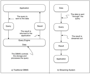
This inverts the traditional data management model by assuming users to be passive and the data management system to be active. Figure 4.3 shows this inversion graphically.
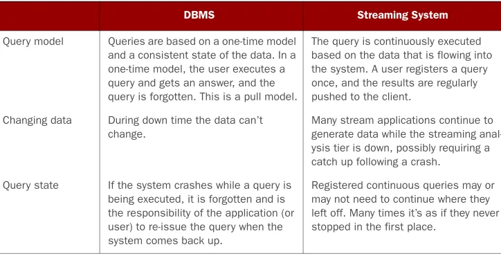
Looking at figure 4.3a, you can see that with the traditional DBMS the query is sent to the data and executed, and the result is returned to the application. In a streaming sys-tem, as illustrated in figure 4.3b, this is model is completely changed and the data is sent “through” the query and the result is then sent to an application. In the case of the streaming system the data is being pulled or pushed through our system in a never-ending stream; this undoubtedly has implications on both the design and the way we query these systems. To give you a better feel for these differences, table 4.1 highlights some of the main differences between a traditional DBMS and streaming system.
If you sit back and think of all the data zipping around you all day long, from the myr-iad of connected devices and appliances to online activity, the questions you could ask and problems you could solve if it all passed through a streaming analysis tier are amazing. Here are some categories and examples to get you going:
Tracking behavior—Imagine being able to provide personalized advertising based on a customer’s location, the weather, and their previous buying habits and preferences. McDonald’s did just this using the VMob platform. According to this ( http://blogs.microsoft.com/iot/2015/01/12/boosting-retail-sales-with-iot-powered-customer-engagement/) case study, McDonald’s in the Nether-lands realized a 700% increase in offer redemptions, and customers using the app returned twice as often and spent on average 47% more.
Improving traffic safety and efficiency—According to the European Commission (http://ec.europa.eu/transport/themes/urban/urban_mobility/index_en.htm), congestion in the European Union (EU) in and around urban areas costs nearly
€100 billion or 1% of EU GDP annually. According to the Federal Highway Administration (http://ops.fhwa.dot.gov/program_areas/reduce-non-cong.htm), 25% of traffic congestion is nonrecurring; it’s caused by traffic incidents. Now
Table 4.1 Comparison of traditional DBMS to streaming system
DBMS Streaming System
Query model Queries are based on a one-time model and a consistent state of the data. In a one-time model, the user executes a query and gets an answer, and the query is forgotten. This is a pull model.
The query is continuously executed based on the data that is flowing into the system. A user registers a query once, and the results are regularly pushed to the client.
Changing data During down time the data can’t change.
Many stream applications continue to generate data while the streaming anal-ysis tier is down, possibly requiring a catch up following a crash.
Query state If the system crashes while a query is being executed, it is forgotten and is the responsibility of the application (or user) to re-issue the query when the system comes back up.
7 Distributed stream processing architecture
imagine you were able to employ roadway vehicle sensors (see http://www .fhwa.dot.gov/policyinformation/pubs/vdstits2007/03.cfm for an introduction); based on our analysis of the traffic data we can provide drivers with updated traf-fic conditions and reroute traftraf-fic accordingly to maximize driving eftraf-ficiency. For real-world examples take a look at Blip Systems (http://www.blipsystems.com/ traffic/); they have examples of how some cities have solved a myriad of traffic problems.
Real-time fraud analytics—Every time a credit card is swiped, a complex series of algorithms must be executed to determine if the attempted transaction is valid or fraudulent. According to FICO (http://www.fico.com/en/node/ 8140?file=5582), there has been a 70% reduction in U.S. fraud losses on credit cards as a percentage of credit card sales since real-time fraud analytics have been deployed.
These examples are just the tip of the iceberg and hopefully have whet your appetite for what’s possible. They also may help you realize that understanding how to build these systems to harness the myriad of data streams available in the world today is becoming an essential skill. But let’s not get ahead of ourselves just yet; we have our work cut out for us learning about the core features of an analysis tier. Let’s begin our journey by discussing the general architecture of a stream-processing system and then move onto the key features and see how each of the features plays a role in your deci-sion to use a particular framework.
4.2
Distributed stream processing architecture
It may be possible to run an analysis tier on a single computer, but the velocity and vol-ume of the data at some point make this a non-viable option. For example, if instead of tracking trending or broken links to articles, imagine we were interested in analyz-ing the performance of a gas turbine in real time to determine if it was functionanalyz-ing correctly. According to General Electric, a single turbine engine can produce approx-imately 1 TB of data per hour. Clearly, using a single computer will quickly become a non-viable option for us. Therefore, we’re going to concentrate on the tools and tech-nologies involved in building a distributed analysis tier. As you survey the technology landscape, you’ll find various technologies designed for stream processing. At the time of this writing the three most popular open source products are Apache Spark Streaming, Apache Storm, and Apache Samza. We’re not going to go into detail on each of them, but we’ll discuss each of them briefly after we go over our generalized streaming architecture so you can see how each fits into it.
A GENERALIZEDARCHITECTURE
If you reflect over the figures for Spark, Storm and Samza, I think you’ll start to see a pattern. They all have the following three common parts:
Separate nodes in the cluster that execute your streaming algorithms.
Data sources that are the input to the streaming algorithms.
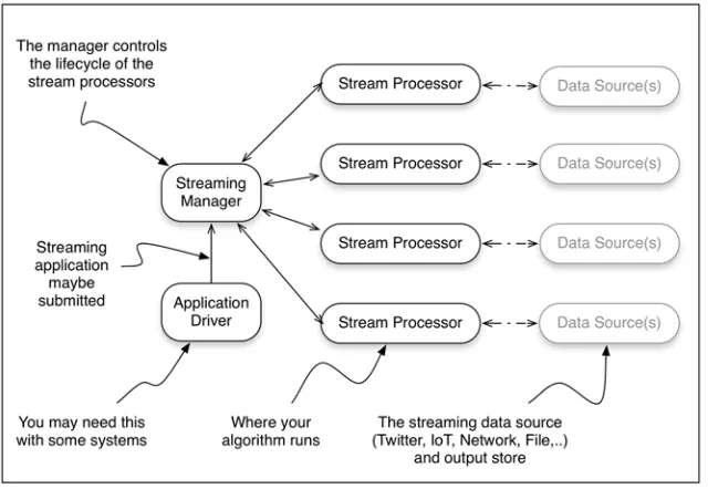
Taking these central ideas and their respective architectures into consideration, we can generalize this into a single common architecture, as shown in figure 4.4.
There are other streaming systems on the market today that have not achieved the same level of popularity as those we discussed in the previous section, and undoubt-edly there will be more in the future. In many cases other products will map onto this common architecture and help in your understanding of how they work. To make sure we’re on the same page, let’s briefly discuss the common architectural pieces shown in figure 4.4.
Application driver—With some streaming systems, this will be the client code that defines your streaming programming and communicates with the streaming manager. For example, with Spark Streaming your client code is broken into two logical pieces: the driver and the streaming algorithm(s) or job. The driver submits the job to the streaming manager, may collect results at the end, and controls the lifetime of your job.
Streaming manager—The streaming manager has the general responsibility of getting your streaming job to the stream processor(s); in some cases it will con-trol or request the resources required by the stream processors.
Stream processor—This is really where the rubber meets the road, the place where your job actually runs. Although this may take many shapes based on the
9 Distributed stream processing architecture
streaming platform in use, the job remains the same: to execute the job that was submitted.
Data source(s)—This represents the input and potentially the output data from your streaming job. With some platforms your job may be able to ingest data from multiple sources in a single job, whereas others may only allow ingestion from a single source. One thing that may not be obvious from the architectures is where the output of the jobs goes. In some cases you may want to collect the data in your driver, whereas in other cases you may wish to write it out to a dif-ferent data source to be used by another system or as input for another job.
Now that you have an understanding of the various architectures and have boiled them down to our common architecture, let’s go back to our example of monitoring the performance of gas turbines to determine if they’re functioning correctly and map that to our common architecture. In figure 4.5 you can see our common archi-tecture (simplified so it is less busy) with our business problem mapped to it.
I realize that this may have been a lot to digest, so take a moment to see if you can map your business problem to the common architecture we’ve derived. When you’re ready, we’ll discuss the architecture of the three major streaming systems and then go a little deeper and discuss some of the key features you’ll want to think about when choosing a stream-processing framework.
APACHE SPARK STREAMING
Apache Spark Streaming, often just called Spark Streaming, is built on Apache Spark, as depicted in figure 4.6.
As you’ll notice, there are various other features built on top of Apache Spark. Apache Spark is becoming the de facto platform for general-purpose distributed com-putation. It provides support for multiple languages (Java, Scala, Python, and R) and
at the time of this writing has the following high-level tools built on top of it: Spark Streaming, MLlib (Machine Learning), SparkR (integration with R), and GraphX (for graph processing). Outside the normal project documentation, a great resource to start learning more about Spark is Marko Bonac´i and Petar Zecˇevic´’s book Spark in Action (https://www.manning.com/books/spark-in-action). Keeping our focus on Spark Streaming, let’s take a look at its overall architecture, shown in figure 4.7.
Let’s discuss the general flow of how things work so that you have an understand-ing of its basic architecture. Startunderstand-ing from the left in the figure we have our program, which contains what is called a Spark StreamingContext; collectively this is commonly referred to as the driver. Without diving into the details, the Spark StreamingContext contains all of the logic to be able to keep track of incoming data, set up the stream-ing jobs, schedule them on the Spark workers, and execute the jobs. You may notice here that we’re talking about jobs and not a stream. The reason for this is that Spark and subsequently Spark Streaming operate on batches of work. In the case of Spark Streaming these batches represent data over a period of time and can be scheduled to
Figure 4.6 Apache Spark Streaming with the basic Spark stack
11 Distributed stream processing architecture
run at frequencies less than half a second. A job in Spark Streaming is just the logic of your program that’s bundled up and passed to the Spark workers. If you’ve read about or worked with Hadoop Map Reduce, this is the same concept. Moving to the middle of figure 4.7 you see the Spark workers; these run on any number of computers (from one to thousands) and are where your job (your streaming algorithm) is executed. As you’ll notice, they receive data from an external data source and communicate with the Spark StreamingContext that’s running as part of the driver.
APACHE STORM
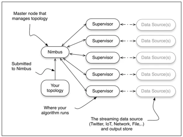
Apache Storm is tuple-at-a-time stream-processing framework designed for real-time processing of data streams. There are many features to Storm, which we won’t cover in detail. For great references to learn more about Storm see Sean Allen, Peter Pathi-rana, and Matthew Jankowski’s Storm Applied (Manning 2013). The overall architec-ture for Storm is shown in figure 4.8.
Looking at figure 4.8, you can see that from a high-level it’s very similar to Spark Streaming or perhaps a Hadoop cluster if you change Nimbus to a job tracker and the supervisors to data nodes. Unlike Hadoop and Spark that use the term job to describe the unit of work, with Storm the term topology is used instead. The reasoning behind this is that a job will eventually finish whereas a topology will run forever. Let’s not get bogged down by this semantic sugar; at the end of the day they both represent a way to deploy your program to the worker nodes. With this definition in mind, let’s walk through figure 4.8 and discuss the different pieces.
Starting on the bottom left you can see the topology; this is submitted to a compo-nent called Nimbus. Nimbus is in charge of deciding how the topology is deployed across the supervisors, assigns different tasks to the supervisors, and monitors the entire system for failures. Moving to the middle of the figure you will see the supervi-sor nodes; these are where your topology actually runs. On the right is the data source; this just represents the data that will be ingested by the running topology.
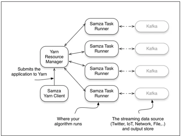
APACHE SAMZA
The streaming model with Apache Samza is slightly different in that it provides a stage-wise stream processing framework. To do this it leverages two prominent tech-nologies found in the Big Data space, those being Apache Yarn and Apache Kafka. We won’t spend much time talking about those technologies, but we will discuss them briefly as they relate to the high-level Samza architecture shown in figure 4.9.
As we’ve done with the others, let’s take a minute to walk through this architecture. One of the things that I think will jump right out at you is the new technologies that appear, in particular Yarn and Kafka. Yarn is a cluster manager designed to handle resource management and job scheduling/monitoring. I know that’s a mouthful; just think of it this way: the resource management part is responsible for allocating resources (CPUs, memory, disk, network, and so on) for the various applications that are running on a cluster of computers. The job scheduling/monitoring aspect is responsible for actually running the job on the cluster. When looking at figure 4.9 you can see that the Samza Yarn client makes a request to the Yarn resource manager asking that the requested
13 Key features of stream-processing frameworks
resources be allocated for the Samza application to run. Subsequently after some resource negotiation, the Samza task runners are executed in various nodes in the clus-ter. This is intentionally simplified, because focusing on the Yarn specifics at this time doesn’t add value to our discussion and is subject to change as the project matures. Moving to the center of the figure you can see our Samza tasks running. In this case all input and output to our Samza tasks will be done using Apache Kafka. Apache Kafka is a technology that squarely fits into our discussion in chapter 3 on the message queueing tier and a technology we’ll revisit in future chapters. For now you can think of it as a high-speed data store that our streaming tasks will read from and write to. Some great resources to learn more about Yarn are Alex Holme’s Hadoop in Practice, Second Edition (Manning 2014) and Chuck Lam, Mark Davis, and Ajit Gaddam’s book Hadoop in Action, Second Edition (Manning 2014). To find the latest information on Apache Samza, please visit http://samza.apache.org.
4.3
Key features of stream-processing frameworks
Many different stream-processing frameworks can be used in the analysis tier of our streaming data architecture. When we boil them down there are a handful of key fea-tures that we want to pay special attention to when comparing them and deciding if they’re suitable for solving our business problem. In this section we’ll discuss the key features you need to pay special attention to; make sure you understand each of them and can apply this knowledge when selecting the stream-processing framework you’ll use in your streaming data architecture.
4.3.1 Message delivery semantics
In chapter 3 you learned about message delivery semantics in respect to the message queueing tier and the producers, brokers, and consumers. This time we focus our dis-cussion of message delivery semantics on the analysis tier. The definitions don’t change, but you’ll notice that the implications are a little different. First, let’s refresh your memory on the definitions of the different guarantees:
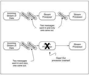
At-most-once—A message may get lost, but it will never be processed a second time.
At-least-once—A message will never be lost, but it may be processed more than once.
Exactly-once—A message is never lost and will be processed only once.
Figure 4.10 shows at-most-once semantics with the two failure scenarios: a message dropping and a streaming task processor failing. The second scenario, a streaming task processor failing, will also result in message loss until a replacement processor comes online.
At-most-once is the simplest delivery guarantee a system can offer; no special logic is required anywhere. In essence, if a message gets dropped, a stream processor crashes, or the machine that a stream processor is running on fails, the message is lost. At-least-once increases the complexity because the streaming system must keep track of every message that was sent to the stream processor and an acknowledgement that it was received. If the streaming manager determines that the message was not processed (perhaps it was lost or the stream processor didn’t respond within a given time boundary), then it will be resent. It’s important to keep in mind that at this level of messaging guarantee your streaming job may be sent the same message multiple times. Therefore, your streaming job must be idempotent, meaning that every time your streaming job receives the same message, it produces the same result. If you keep this in mind when designing your streaming jobs, then you will be able to handle the duplicate-messages situation.
Exactly-once semantics ratchets up the complexity a little more for the stream-pro-cessing framework. Besides the bookkeeping that it must keep for all messages that have been sent, it now must also detect and ignore duplicates. With this level of guar-antee your streaming job no longer has to worry about dealing with duplicate messages;
15 Key features of stream-processing frameworks
it only has to make sure it responds with a success or failure after a message is processed. Even though it’s not required of your streaming job to be idempotent with this level of messaging guarantee, I highly recommend that you approach all of your streaming jobs with the expectation that they should be idempotent. It will make troubleshooting and reasoning about them much easier.
You may be wondering which of these guarantees you need; in reality it will depend on the business problem you’re trying to solve. Let’s take our example from earlier: the turbine engine monitoring system. Remember that for this system we want to constantly analyze how our turbine engine is performing so we can predict when a failure may occur and pre-emptively perform maintenance. Earlier we said our tur-bines produce approximately 1 TB of data every hour, which may not seem like a lot of data, but keep in mind that is one turbine and we’re monitoring thousands to be able to predict when a failure may occur. What do you think; do we need to ensure we don’t lose a single message? We may, but it would be worth investigating if our predic-tion algorithm needs all of the data or not. If it can perform adequately if data is miss-ing, then I’d choose the least complex guarantee first and work from there.
What if instead your business problem involved making a financial transaction based on a streaming query? Perhaps you operate an ad network and you provide real-time billing to your clients. In this case you’d want to ensure that the streaming system you choose provides exactly-once semantics.
I think you get the hang of it and can apply this to your business problem. Now let’s move on to talk about state management.
STATEMANAGEMENT
Once your streaming analysis algorithm becomes more complicated than just using the current message without dependencies on any previous messages and/or external data, you’ll need to maintain state and will likely need the state management services provided by your framework of choice. Let’s take a simple example that we can work with to help you understand where and perhaps how state needs to be managed.
Pretend you’re the marketing manager for a large e-commerce site and you want to know the number of page views per hour for each visitor.
I know you’re thinking “an hour” that can be done in a batch process. We’re not going to worry about that right now; instead, let’s focus on the implied state you must keep to satisfy this business question. Figure 4.11 shows how your streaming task pro-cessors would be organized to answer this question.
state in memory may be acceptable. But in many business cases life is not so simple and you do need to worry about managing state. To help in these scenarios, many stream-processing frameworks provide state management features that you can leverage.
The state management facilities provided by various systems naturally fall along a complexity continuum, as shown in figure 4.12.
The continuum starts on the left with a naïve in-memory-only choice similar to what we used earlier and progresses to the other end of the spectrum with systems that provide a queryable persistent state that’s replicated. If you find yourself saying “these seem like two totally different slants on state management,” you’re not alone. The solutions on the low-complexity side only solve the problem of maintaining the state of a computation in the face of failures. For the simple operations of keeping a run-ning count current and not losing track of the current value in the face of failure, these systems are a great fit. On the other end of the spectrum, the frameworks that offer state management by way of a replicated queryable persistent store help you answer much different and more complicated questions. With these frameworks you
Figure 4.11 Simple example of counting page views per user over an hour
17 Key features of stream-processing frameworks
can join different streams of data together. For example, imagine you were running an ad-serving business and you wanted to track two things: the ad impression and the ad click. It’s reasonable that the collection of this data would result in two streams of data, one for ad impressions and one for ad clicks. Figure 4.13 shows how these streams and your streaming job would be set up for handling this.
In this example the ad impressions and ad clicks arrive in two separate streams; because the ad clicks will lag the ad impressions, we’ll join the two streams and then count by the user ID. Because of the lag in the ad click stream, using a stream-process-ing framework that persists the state in a replicated queryable data store enables us to join the two streams and produce a single result. I think you’ll agree that being able to join streams by leveraging the state management facilities of a stream-processing framework is quite a bit different than just making sure the current value of an aggre-gation is persisted. If you give some more thought to this example, I’m sure you’ll come up with other ideas of how you can join more than one stream of data. It’s a fas-cinating topic and something we’ll look at in more depth in our next chapter. For now, let’s continue on to the next feature you need to understand when choosing a stream-processing framework.
FAULTTOLERANCE
It’s nice to think of a world where things don’t fail, but in reality it’s not a matter of if
things will fail but only a matter of when. A stream-processing framework’s ability to keep going in the face of failures is a direct result of its fault tolerance capabilities. When we consider all of the pieces involved in stream-processing, there are quite a few places where it can fail. Let’s take another look at the pieces involved and use figure 4.14 to identify all of the failure points.
In figure 4.14 we’ve identified seven points of failure in a very simple stream-process-ing data flow. Go through them and make sure you understand what you’ll need from a stream-processing framework in respect to fault tolerance:
1 Incoming stream of data—In all fairness the message queueing tier won’t be under the control of the stream-processing framework, but there is the poten-tial for the message queueing system to fail, in which case the stream-processing framework must respond gracefully and not fail if data is not available or the resource is not available.
2 Network carrying input stream—This is something that the stream-processing framework can’t control, but it needs to handle the disruption gracefully.
3 Stream processor—This is where your code is running and it should be under supervision of the stream-processing framework. If something goes wrong here, perhaps your software fails or the machine it’s running on fails, then the streaming manager should take steps to restart the processor or move the pro-cessing to a different machine.
4 Connection to output destination—The stream task manager may not be able to control the network path to the output, but it should be able to control the flow of data from the last stream processor so that it doesn’t become overwhelmed by network back pressure or fail if the network or destination is unavailable.
5 Output destination—This would not be under the direct supervision of the stream task manager, but its failing could impact the processing of the stream and therefore it needs to be considered.
6 Streaming manager—If this fails, then you end up with a situation that’s often referred to as “running headless.” This refers to the situation where the stream processors would continue to run without being supervised by the streaming
19 Key features of stream-processing frameworks
manager. Thus if this is component fails, there’s no supervisor for the data flow and the stream processors—no new ones can be started or failed ones recovered.
7 Application driver—This comes in two flavors. With the first, the application driver does nothing more than submit the streaming job to the streaming man-ager—we’re not worried about this type. The second flavor is where the applica-tion driver logically contains the streaming manager and in turn is subject to the same risk as the streaming manager.
Now that you understand what you need from a stream-processing framework, let’s go through how these problems are solved or could be solved. First, let’s boil our prob-lem down a bit. If we look the previous list, we can eliminate the incoming stream and output destination availability from the concerns of the streaming framework. It should go without saying that the streaming framework must not fail if there are fail-ures with the input or output destinations. But for this discussion we won’t consider those aspects to be fault tolerance related. Now if we take the list and consolidate it down to the common elements, we end up with the following:
Data loss—This covers data lost on the network and also the stream processor or your job crashing and losing data that was in memory during the crash.
Loss of resource management—This covers the streaming manager and your appli-cation driver in the event you have one.
If you recall our discussion of fault tolerance in chapter 3, you may remember that we discussed ways to prevent data loss. When it comes to stream-processing frameworks, all of the common techniques for dealing with failures involve some variant of replica-tion and coordinareplica-tion. A common approach would be for the stream manager to rep-licate the state of a computation (the state of your streaming job) onto different stream processors. If there’s a failure, then the streaming manager must coordinate the replicas in order to recover properly from failures. It’s common for fault-tolerance techniques to be designed with a tolerance up to a predefined number of simultane-ous failures, in which case you’ll hear of a system being called k-fault tolerant, where k represents the number of simultaneous failures.
streaming job is running on. But this allows for quick failover, resulting in very little dis-ruption. For some applications, such as an intrusion-detection system that has low-latency requirements at all times, the extra resource cost may be justifiable.
The second approach is known as rollback recovery. In this approach, the stream processor periodically packages the state of our computation into what is called a checkpoint, and it copies the checkpoint to a different stream processor node or a nonvolatile location such as a disk. Between checkpoints, the stream processor has to keep track of the computation. Given the relative high latency of disks, once they’re introduced the latency of our streaming computation will go up. It therefore may not be unreasonable for a stream-processing framework to instead decide to take the approach of copying the checkpointed state to other stream processor nodes and also maintain logs in memory. In this case if a stream processor fails, the stream manager would need to reconstruct the state from the most recent checkpoint and replay the log to recover the exact pre-failure state of the streaming job. Compared to the first approach, this approach has a lower overhead but it’s more expensive in terms of time to recover when a failure does happen. This approach is useful in situations where fault tolerance is important and rare moderate latencies are acceptable.
As you investigate which stream-processing framework to use to solve your business problem, you’ll find that if they offer fault-tolerance they’ll all be some variant on these two common approaches. If you’re interested in taking a deeper dive into either of these approaches, you may find the following articles of interest: Elnozahy, Alvisi, Wang, and Johnson’s “A Survey of Rollback-Recovery Protocols in Message-Passing Systems”1 and Schneider’s “Implementing Fault-Tolerant Services Using the State
Machine Approach: A Tutorial.”2
4.4
Summary
In this chapter we took a dive into the common architecture of stream-processing frameworks you’ll find when surveying the landscape, and we went over the core fea-tures that you need to consider.
You learned
About the common architecture of stream-processing frameworks
What message delivery semantics mean for this tier
What state is and how it can be managed
What fault tolerance is and why you need it
Streaming Data introduces the concepts and require-ments of streaming and real-time data systems. Through this book you’ll develop a foundation to understand the challenges and solutions of building in-the-moment data systems before committing to spe-cific technologies. Using copious diagrams, this book systematically builds up the blueprint for an in-the-moment system concept by concept. Although code may occasionally appear in examples, this book focuses on the big ideas of streaming and real-time data sys-tems rather than the implementation details.
Many of the technologies discussed in the book— Spark, Storm, Kafka, Impala, RabbitMQ, etc.—are covered individually in other books. As you read, you’ll get a clear picture of how these technologies work individu-ally and together, gain insight on how to choose the correct technologies, and dis-cover how to fuse them together to architect a robust system.
What’s inside
Understand and architect a complete system for collecting and analyzing data in real time
Harness the “Internet of Things” by handling live data from billions of devices
Use the specific functions of each tier of an in-the-moment system to solve real business problems
Combine emerging technologies like Spark, Storm, Kafka, RabbitMQ, and Web-Sockets
Integrating and extending the Lambda architecture into a complete system
A
s applications grow in size and complexity, the impact of unanticipated error or application failure looms large. Reactive design introduces new ways of thinking about managing failure. The following chapter provides an overview of fault tolerance and recovery patterns, which, arguably, are neglected during the development of many applications. In the worst cases, this can lead to cascading failures that render an entire system unusable.23
Chapter 12 from
Reactive Design Patterns
by Roland Kuhn
with Brian Hanafee and Jamie Allen
Fault tolerance
and recovery patterns
In this chapter you will learn how to incorporate the possibility of failure into the design of your application. We will demonstrate the patterns in the concrete use-case of building a resilient computation engine that allows batch job submissions and their execution on elastically provisioned hardware resources. We build upon what we learned in chapters 6 and 7, so you might want to refresh your understand-ing of those.
We start out with considering a single component and its failure and recovery strategies, then we build up more complex systems by hierarchical composition as well as client–server relationships. In particular we discuss the following patterns:
The Simple Component Pattern (a.k.a. the Single Responsibility Principle)
The Error Kernel Pattern
The Let-It-Crash Pattern
The Circuit Breaker Pattern
12.1
The Simple Component Pattern
“A component shall do only one thing, but do it in full.”
This pattern derives from the Single Responsibility Principle that was formulated by De Marco in his 1979 book Structured analysis and system specification (Yourdon, New York). In its abstract form it demands to “maximize cohesion and minimize coupling,” applied to object-oriented software design it is usually stated as “a class should have only one reason to change.”1
From the discussion of divide et regna in chapter 6 we know that in order to break a large problem up into a set of smaller ones, we can find help and orientation by look-ing at the responsibilities that the resultlook-ing components will have. Applylook-ing the pro-cess of responsibility division recursively allows us to reach any desired granularity and results in a component hierarchy that we can then implement.
12.1.1 The Problem Setting
As an example consider a service that offers computing capacity in a batch-like fash-ion: users submit jobs to be processed, stating a job’s resource requirements and including an executable description of the data sources and the computation that is to be performed. The service will have to watch over the resources that it manages: it will have to implement quotas for the resource consumption of its clients and sched-ule jobs in a fair fashion. It will also have to persistently queue the jobs that it accepts such that clients can rely upon their eventual execution.
THE TASK
Your mission is to sketch the components that make up the full batch service, noting for each one what exactly its responsibility is. Start from the top-level and work your way downwards until you reach components that are concrete and small enough so that you could task teams with implementing them.
12.1.2 Applying the Pattern
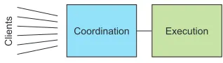
We can immediately conclude that the service implementation will be made up of two parts: one that does the coordination and that the clients communicate with, and another that will be responsible for the actual execution of the jobs; this is shown in figure 12.1. In order to make the whole service elastic, the coordinating part would tap into an external pool of resources and dynamically spin up or down executor instances. We can see that the coordination will be a rather complex task and there-fore we want to break it up further.
To follow the flow of a single job request through this system, we start with the job sub-mission interface that is offered to clients. This part of the system needs to present a net-work endpoint that clients can contact; it needs to implement a network protocol for
1 Uncle Bob, “Principles of OOD” (May 11, 2005;
http://butunclebob.com/ArticleS.UncleBob.Principles-OfOod)
Clients
Coordination Execution
25 The Simple Component Pattern
this purpose and it will interact with the rest of the system on behalf of the clients. We could break up responsibility even finer along these lines, but for now let us consider this aspect of representing clients within the client as one responsibility; the client interface will thus be our second dedicated component.
Once a job has been accepted and the client has been informed by way of an acknowledgement message our system must ensure that eventually the job will be exe-cuted. This can only be achieved by storing the incoming jobs on some persistent medium and we might be tempted to place this storage within the client interface component. But we can already anticipate that other parts of the system will have to access these jobs, for example in order to start their execution. This means that in addition to representing the clients this component would assume responsibility for making job descriptions accessible to the rest of the system, which is in violation of the single responsibility principle.
Another temptation might be to share the responsibility for the handling of job descriptions between the interested parties—at least the client interface and the job executor as we may surmise—but that will also greatly complicate each of these com-ponents, as they will now have to coordinate their actions, running counter to the Simple Component Pattern’s goal. It is much simpler to keep one responsibility within one component and avoid the communication and coordination overhead that comes with distributing it across multiple components. Besides these runtime con-cerns we also need to consider the implementation: sharing the responsibility means that one component needs to know about the inner workings of the other, so their development needs to be tightly coordinated as well. These are the reasons behind the second part of “do only one thing, but do it in full.”
This leads us to identify the storage of job descriptions as another segregated responsibility of the system and thereby as the third dedicated component. A valid interjection at this point is that the client interface component might well benefit from persisting the incoming jobs within its own responsibility, this would allow shorter response times for the job submission acknowledgement and it also makes the client interface independent from the job storage component in case of temporary unavailability. However, such a persistent queue would only have the purpose of even-tually delivering accepted jobs to the storage component, who then will take responsi-bility of them. Therefore these notions are not in conflict with each other, we might implement both if system requirements demand it.
Clients
Coordination
Storage Client
interface
Job
scheduling Execution
Taking stock, by now we have identified the client interface, the job storage, and the job executor as three dedicated components with non-overlapping responsibilities. What remains to be done is to figure out which jobs to run in what order, we call this part “job scheduling.” The current state of our system’s decomposition is shown in fig-ure 12.2; now we apply this pattern recursively until the problem is broken up into simple components.
Probably the most complex task in the whole service is to figure out the execution schedule for the accepted jobs, in particular when prioritization or fairness is to be implemented between different clients that share a common pool of resources—the corresponding allocation of computing shares are usually a matter of intense discus-sion between competing groups of people.2 The scheduling algorithm will need to
have access to job descriptions in order to extract scheduling requirements (maxi-mum running time, possible expiry deadline, which kind of resources are needed, etc.), so this is another client of the job storage component.
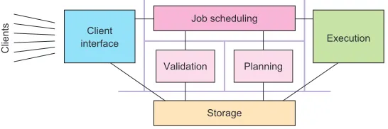
It takes a lot of effort—both for the implementation and at runtime—to plan the execution order of those jobs that are accepted for execution, and this task is inde-pendent from deciding which jobs to accept. Therefore it will be beneficial to sepa-rate the responsibility of job validation into its own component. This also has the advantage of removing the rejected tasks before they become a burden for the sched-uling algorithm. The overall responsibility of job schedsched-uling now consists of two com-ponents, but its overall function should still be represented consistently to the rest of the system. For example, the executors need to be able to retrieve the next job to run at any given time independently of whether there is a scheduling run in progress or not. For this reason we place the external interactions in an overall scheduling com-ponent of which the validation and planning responsibilities are delegated to sub-components. The resulting split of responsibilities for the whole system is shown in figure 12.3.
12.1.3 The Pattern Revisited
The goal of this pattern is to implement the Single Responsibility Principle and we did that by considering the responsibilities of the overall system at the highest level—cli-ent interface, storage, scheduling, execution—and separating these into dedicated
2 The authors have some experience with such allocation between different groups of scientists competing for
data analysis resources in order to extract the insights they need for academic publications.
Clients
Client interface
Job scheduling
Storage
Execution Validation Planning
27 The Error Kernel Pattern
components, keeping an eye on their anticipated communication needs. We then dived into the scheduling component and repeated the process, finding that there are sizable and non-overlapping responsibilities which we split out into their own sub-components. This left the overall scheduling responsibility in a parent component because we anticipate coordination tasks that will be needed independently of the sub-components’ functions.
By this process we arrived at segregated components that can be treated indepen-dently during the further development of the system. Each of these has one clearly defined purpose and each core responsibility of the system lies with exactly one ponent. Though the overall system and the internals of any component may be com-plex, the Single Responsibility Principle yields the simplest division of components to further work on—it frees us from always having to consider the whole picture when working on smaller pieces. This is its quintessential feature: it addresses the concern of system complexity.
Additionally, following the Simple Component Pattern simplifies the treatment of failures as we will exploit in the following two patterns.
12.1.4 Applicability
This is the most basic pattern to follow and it is universally applicable. Its application may lead you to a fine-grained split of your problem or to the realization that you are dealing with only one single component—the important part is that afterward you know whyyou chose your system structure as you did. It helps all later phases of the design and implementation to document and remember this, because when questions come up later of where to place certain functionality in detail you can let yourself be guided by the simple question of “what is its purpose?” The answer will directly point you toward one of the responsibilities you identified, or it will send you back to the drawing board in case you forgot to consider it.
It is important to remember that this pattern is meant to be applied in a recursive fashion, making sure that none of the identified responsibilities remain too complex or high-level. One word of warning, though: once you start dividing up components hierarchically it is easy to get carried away and go too far—the goal is simple compo-nents that have a real responsibility, not trivial compocompo-nents without an individual rea-son to exist.
12.2
The Error Kernel Pattern
“In a supervision hierarchy keep important application state or functionality near the root while delegating risky operations towards the leaves.”
Pattern will frequently leave you in this position, hence it pays to familiarize yourself well with the Error Kernel.
This pattern has been established in Erlang programs for decades3and was one of
the main reasons that inspired Jonas Bonér to implement an Actor framework— Akka—on the JVM. The name “AKKA” was originally conceived as the palindrome of “Actor Kernel,” referring to this core design pattern.
12.2.1 The Problem Setting
From the discussion of hierarchical failure handling in chapter 7 we know that each component of a reactive system is supervised by another component that is responsi-ble for its lifecycle management. This implies that if the supervisor component fails then all its subordinates will be affected by the subsequent restart, resetting everything to a known good state and potentially losing intermediate updates. If the recovery of important pieces of state data is expensive then such a failure will lead to extensive service downtimes, a condition that reactive systems aim to minimize.
THE TASK
Consider each of the six components identified in the previous example as a failure domain and ask yourself which component should be responsible for reacting to its failures as well as which components will be directly affected by them. Summarize your findings by drawing the supervision hierarchy for the resulting system architecture.
12.2.2 Applying the Pattern
Since recovering from a component’s failure implies the loss and subsequent recre-ation of its state, we shall look for opportunities to separate likely points of failure from the places where important and expensive data are kept. The same applies to pieces that provide services that shall be highly available: these should not be obstructed by frequent failure nor long recovery times. In the example we identified the following disparate responsibilities:
Communication with clients (accepting jobs and delivering their results)
Persistent storage of job descriptions and their status
Overall job scheduling responsibility
Validation of jobs against quotas or authorization requirements
Job schedule planning
Job execution
Each of these responsibilities benefits from being decoupled from the rest. For exam-ple the communication with clients should not be obstructed by a failure of the job scheduling logic, just as client-induced failures should not affect the currently run-ning jobs. The same reasorun-ning applies to the other pieces analogously. This is another reason in addition to the single responsibility principle for considering them as dedi-cated components as shown again in figure 12.4.
3 The Ericsson AXD301’s legendary reliability is attributed in part to this design pattern and its success
29 The Error Kernel Pattern
The next step is to consider the failure domains in the system and ask ourselves how each of them should recover and how costly that process will be. To this end we follow the path by which a job travels through the system.
Jobs enter the service through the communication component, which speaks an appropriate protocol with the clients, maintaining protocol state and validating inputs. The state that is kept is short-lived, tied to the communication sessions that are currently open with clients. When this component fails, affected clients will have to re-establish a session and possibly send commands or queries again, but our component does not need to take responsibility for these activities. In this sense it is effectively stateless—the state that it does keep is ephemeral and local. Recovery of such compo-nents is trivially done by just terminating the old and starting the new runtime instance.
Once a job has been received from a client, it will need to be persisted, a responsi-bility that we placed with the storage component. This component will have to allow all other components to query the list of jobs, selecting them by current status or cli-ent account and holding all necessary meta-information. Apart from caches for more efficient operation, this component does not hold any runtime state; its function is only to operate a persistent storage medium, therefore it can easily be restarted in case of failure. This assumes that the responsibility of providing persistence will be split out into a sub-component—which today is a likely approach—that we would have to consider as well. If the contents of the persistent storage become corrupted then it is a business decision whether to implement (partial) automatic resolution of these cases or leave it to the operations personnel. Automatic recovery would presumably interfere with normal operation of the storage medium and would therefore fall into the storage component’s responsibility.
The next stop of a job’s journey through the batch service is the scheduling com-ponent. At the top level this one has the responsibilities of applying quotas and resource request validation, as well as providing the executor component with a queue of jobs to pick up. The latter is crucial for the operation of the overall batch service: without it the executors would run idle and the system would fail to perform its core function. For this reason we place this function at the top of the scheduling
Clients
Client interface
Storage
Execution
Validation Planning Job scheduling
component’s priorities and correspondingly at the root of its sub-component hierarchy as shown in figure 12.5.
While applying the Simple Component Pat-tern we identified two sub-responsibilities of the scheduling component. The first is to vali-date jobs against policy rules like per-client quotas4 or general compatibility with the
cur-rently available resource set—it would not do to accept a job that needs 20 executor units when only 15 can be provisioned. Those jobs that pass validation from the input to the second sub-component that performs the job schedule planning for all cur-rently outstanding and accepted jobs. Both of these responsibilities are task-based; they are started periodically and then either complete successfully or fail. Failure modes include hardware failures as well as not terminating within a reasonable time frame. In order to compartmentalize possible failures, these tasks should not directly modify the persistent state of jobs or the planned schedule but instead report back to their parent component who then takes action, be that notifying clients (via the client interface component) of jobs that failed their submission criteria or updating the internal queue of jobs to be picked next.
Whereas restarting the sub-components proved to be trivial, restarting the parent scheduling component is more complex—it will need to initiate one successful sched-ule planning run before it can reliably resume performing its duties. Therefore we keep the important data and the vital functionality at the root and delegate the poten-tially risky tasks to the leaves. Here again we note that the Error Kernel Pattern con-firms and reinforces the results of the Simple Component Pattern: we frequently find that the boundaries of responsibilities and failure domains coincide and that their hierarchies match as well.
Once a job has reached the head of the scheduler’s priority queue it will be picked up for execution as soon as computing resources become available. We have so far considered execution to be an atomic component, but when considering failure we come to the conclusion that we will have to divide its function: the executor needs to keep track of which job is currently running where and it will also have to monitor the health and progress of all worker nodes. The worker nodes are those components that upon receiving a job description will interpret the contained information, contact data sources, and run the analysis code that was specified by the client. Clearly the fail-ure of each worker shall be contained to that node and not spread to other workers or the overall executor, which implies that the execution manager supervises all worker nodes as shown in figure 12.6.
4 For example one might want to limit the maximal number of jobs queued by one client—both in order to
protect the scheduling algorithm and to enforce administrative limits.
Job scheduling
Parent of...
Planning Validation
31 The Error Kernel Pattern
If the system will be elastic, the executor will also make use of the external resource provision mecha-nism in order to create new worker nodes or shut down unused ones. The execution manager is also in the position to make the decision to enlarge or shrink the worker pool, because it naturally moni-tors the job throughput and it can easily be informed about the current job queue depth— another approach would be to let the scheduler decide the desired pool size. In any case it is the
executor that holds the responsibility of starting, restarting, or stopping worker nodes since it is the only component that knows when it is safe or required to do so.
Analogous to the client interface component, the same reasoning applies that the communication with the external resource provision mechanism should be isolated from the other activities of the execution manager. A communication failure in that regard should not keep jobs from being assigned to already running executor instances or job completion notifications from being processed.
The execution of the job is the main purpose of the whole service, but the journey of our job through the components is not yet complete. After the assigned worker node has informed the manager about the completion status, this result needs to be sent back to the storage component in order to be persisted. If the job’s nature was such that it must not be run twice, then the fact that the execution was about to start must also have been persisted in this fashion; in this case a restart of the execution manager will need to include a check of which jobs were already started but not yet completed prior to the crash, and corresponding failure results will have to be gener-ated. In addition to persisting the final job status, the client will need to be informed about the job’s result, which completes the whole process.
Now that we have illuminated the function and relationship of the different com-ponents, we recognize that we have omitted one in the earlier list of responsibilities. The service itself needs to be orchestrated, composed from its parts, supervised, and coordinated. We need one top-level component that creates the others and arranges for jobs and other messages being passed between them. In essence it is this compo-nent’s function to oversee the message flow and thereby the business process of the service. This component will be top-level because of its integrating function that is needed at all times, even though it may be completely stateless by itself. The complete resulting hierarchy is shown in figure 12.7.
Worker
Resource pool interface Execution
12.2.3 The Pattern Revisited
The essence of what we did in the preceding example can be summarized in the fol-lowing strategy: after applying the Simple Component Pattern, pull important state or functionality towards the top of the component hierarchy, and push activities that carry a higher risk for failure downwards towards the leaves. It is expected that the responsibility boundaries will coincide with failure domains and that narrower sub-responsibilities will naturally fall towards the leaves of the hierarchy. This process may lead you to introduce new supervising components that tie together the functionality of components that are otherwise siblings in the hierarchy, or it might guide you towards a more fine-grained component structure in order to simplify failure han-dling or decouple and isolate critical functions to keep them out of harm’s way. The quintessential function of this pattern is to integrate the operational constraints of the system into its responsibility-based problem decomposition.
12.2.4 Applicability
The Error Kernel Pattern is applicable if any of the following are true:
Does your system consist of components that have different reliability require-ments?
Do you expect components to have significantly different failure probabilities and failure severities?
Does the system have important functionality that it must provide as reliably as possible while also having components that are exposed to failure?
Is there important information kept in one part of the system that is expensive to recreate while other parts are expected to fail frequently?
The Error Kernel Pattern is not applicable if:
No hierarchical supervision scheme is used
The system is a Simple Component
All components are either stateless or tolerant to data loss
Worker
Resource pool interface Execution Job scheduling
Batch job service
Storage Client interface
Planning Validation
33 The Let-It-Crash Pattern
We will discuss the second kind of scenarios in more depth in the next chapter when presenting the Active–Active Replication Pattern.
12.3
The Let-It-Crash Pattern
“Prefer a full component restart to internal failure handling.”
In chapter 7 we discussed “principled failure handling,” noting that the internal recovery mechanisms of each component are limited because they are not sufficiently separated from the failing parts—everything within a component can be affected by a failure. This is especially clear for hardware failures that take down the component as a whole, but it is also true for corrupted state that is the result of some programming error that is only observable in rare circumstances. For this reason it is necessary to delegate failure handling to a supervisor instead of attempting to solve it within the component itself.
This approach is also called crash-only software.5 The idea is that transient but rare
failures are often very costly to diagnose and fix, making it preferable to recover a working system by rebooting parts of it. This way of hierarchical restart-based failure handling allows to greatly simplify the failure model and at the same time leads to a more robust system that even has a chance to survive failures that were entirely unforeseen.
12.3.1 The Problem Setting
We will demonstrate this design philosophy on the example of the worker nodes that perform the bulk of the work in the batch service whose component hierarchy we developed in the previous two patterns. Each of these is presumably deployed on its own hardware—virtualized or not—that it does not share with other components; ide-ally there is no common failure mode between different worker nodes other than a computing center outage.
The problem that we are trying to solve is that the workers’ code may contain pro-gramming errors that rarely manifest, but when they do they will impede the ability to process batch jobs. Examples of this kind are very slow resource leaks that can go undetected for a long time but will eventually kill the machine; this could be open files, retained memory, background threads, etc. and the leak might not occur every time but could be caused by a rare coincidence of circumstances. Another example is a security vulnerability that allows the executed batch job to intentionally corrupt the state of the worker node in order to subvert its function and perform unauthorized actions within the service’s private network—such subversion often is not completely invisible and leads to spurious failures that should better not be papered over.
5 Both of the following articles are by George Candea and Armando Fox: “Recursive Restartability: Turning the